Robust MRI abnormality detection using background noise removal with polyfit surface evolution

R E S E A R C H

Open Access

Robust MRI abnormality detection using

background noise removal with polyfit surface

evolution

Changjiang Liu

, Irene Cheng

, Anup Basu

and Jun Ye

Abstract

Image segmentation plays a vital role in MRI abnormality detection. This paper presents a robust MRI segmentation method to outline potential abnormality blobs. Thresholding and boundary tracing strategies are employed to remove background noises, and hence, the ROIs in the whole process are set. Subsequently, a polyfit surface evolution is proposed to approximately estimate bias field, which makes segmentation robust to image noises. Simultaneously, customized initial level set functions are devised so as to detect subtle bright and dark blobs which are highly potential abnormality regions. The proposed method improves bias field estimation and level set method to acquire fine segmentation with low computational complexities. Analysis of experimental results and comparisons with existing algorithms demonstrates that the proposed method can segment weak-edged, low-resolution MR brain images, and its performance prevails in accuracy and effectiveness.

Keywords: Magnetic resonance (MR), Segmentation, Abnormality detection, Polyfit, Bias field estimation, Level set method

1 Introduction

With the exploration of magnetic resonance imaging (MRI) technology, dramatic changes have been made in visualization of anatomical structures [1, 2]. MRI is a pow-erful imaging modality driven by its flexibility and sensi-tivity to a broad range of tissue properties [3]. However, a CT scan is best suited for viewing bone injuries, diag-nosing lung and chest problems, and detecting cancers [4, 5]. MRI is used to find other problems, such as tumors, bleeding, injury, blood vessel diseases, and infections. For example, researchers strive to detect brain abnormalities in MR images [6, 7]. In this paper, our goal is to segment MR brain images to assist doctors’ diagnosis.

Intensity inhomogeneity or bias field in MR image, which arises from the imperfections of the image acqui-sition process and manifests itself as slow intensity vari-ation over the image domain [8]. This inherent artifact is

*Correspondence: [email protected] †_{Equal contributors}

1_{Artificial Intelligence Key Laboratory of Sichuan Province, Sichuan Province} University Key Laboratory of Bridge Non-destruction Detecting and Engineering Computing, Zigong, China

2_{Sichuan University of Science and Engineering, 643000 Zigong, China} Full list of author information is available at the end of the article

difficult for a human to perceive. However, many segmen-tation methods are very sensitive to spurious inten-sity variations. In 1986, Haselgrove and Prammer [9] first discussed MRI intensity inhomogeneity correction. However, Haselgrove and Prammer assumed that the position and orientation of the surface coil were known, as obstructed its practical application. In the past two decades, many bias field correction algorithms have been presented. The authors in [8] noted that two main approaches, namely prospective [10–14] and retrospective approaches [15–21], had been applied to minimize the intensity inhomogeneity in MR images. Among these abovementioned methods, Andersen et al. [15] incorporated radio frequency inhomogeneity correc-tion into probabilistic classificacorrec-tion model to particorrec-tion an MR image. In addition, Li et al. [22] proposed a new approach for bias field estimation and tissue segmentation in an energy minimization framework. They mathemati-cally justified that the proposed energy is convex in each of its variables. Quantitative evaluations and comparisons verified its robustness and accuracy. The bias field estima-tion proposed by Li et al. needs no previous knowledge of noise distribution, which makes it more applicable.

However, it is a region-based segmentation method and cannot extract small homogeneous regions as level set methods do.

Image segmentation is a fundamental process in many medical imaging applications [23]. Segmentation methods can be roughly divided into eight categories [24–26]: (a) thesholding approaches, (b) region growing approaches, (c) classifiers, (d) clustering approaches, (e) Markov ran-dom field models, (f ) artificial neural networks, (g) deformable models, and (h) atlas-guided approaches. The level set method, as one of the deformable models, was first introduced to delineate region boundaries by using closed parametric curves [27]. It is able to acquire closed contours of regions from an image, which helps partition of a medical image accurately. The authors in [28–30] con-sidered a two-phase level set formulation, in which only one level set function was used to construct two mem-bership functions to segment the image domain into two disjoint regions. The two-phase level set method can only partition images into two parts, making it unsuitable for multi-class segmentation in some medical applications. Recently, researchers have developed multi-phase level set methods [31, 32], using two or more level set functions to define more than two membership functions, which makes it more practical in medical applications. Li et al. [31] have combined bias field estimation with multi-phase level set method. In this framework proposed by Li’s, the formation of initial level set functions was not mentioned yet. Experimental results show initial level set functions influence final segmentation to some extent, especially in certain small regions. At the same time, bias field estimation in [31] lacks denoising capability as well.

Focusing on noise depression and widely applicable ini-tial level set functions, we import ROI (region of interest), bias field polyfit estimation, and customize initial level set functions to multi-phase level set methods. The main contributions in this paper include:

(1) A coarse to fine segmentation method is proposed. Otsu’s method is employed not only to remove background noise but also to set the ROI for the level set method.

(2) A multi-phase level set method with bias field polyfit estimation is proposed. This method can partly depress image noise latent in tissues.

(3) Customized initial level set functions are formulated. The initial level set functions are widely applicable to detect small tissues in MR images.

This remainder of this paper is organized as follows. We first review MRI bias field estimation and multi-phase level set method in Section 2. Section 3 presents a robust MRI abnormality detection method, including background removal or ROI setting, multi-phase level set

method with bias field polyfit estimation, and customized initial level set functions. Experimental results and com-parison with existing methods are outlined in Section 4. Finally, concluding remarks are given in Section 5.

2 Literature review on MRI bias field estimation and multi-phase level set method

In previous works [8, 22, 31], the model of an MR image has been widely accepted as:

I(x)=b(x)J(x)+n(x) (1) where b(x) is bias field that accounts for the intensity inhomogeneity in the observed image I(x), n(x) is the additive Gaussian noise with zero mean, J(x) is the true image without bias field and noise, andxis a tuple like (x,y)representing image coordinates.

An energy minimization formulation [22] in the image domainfor bias field estimation is defined by:

E(b,J)=

|I(x)−b(x)J(x)|2dx (2) In this paper, the domain of integrationis omitted for simplicity. Obviously, the solution for the multiplicative intrinsic componentsbandJis an ill-posed problem with-out constraints on the variablesbandJ. Thus, Li et al. [22] have made the two following assumptions:

(1) Image domaincan be partitioned into disjoint parts as described below:

=

N

i=1

i, i

j= (i=j),

in whichJ is approximately constantcifor thei th regioni. Furthermore,ciis regarded as class center of fuzzy c-means algorithm [33].

(2) The bias fieldb varies slightly in a small neighborhood region of any pointyon thei th regioni, and leads to the approximate relation in Eq. (2):

b(x)J(x)≈b(y)ci, x∈Oy

i

whereOy{x:|x−y| ≤ρ}.

Furthermore, a non-negative window functionK(y−x) is introduced, beingK(y−x)=0 forx∈/Oy, to represent

the energy function bounded on regionias follows:

Ey=

N i=1

iOy

|I(x)−b(y)ci|2dx

= N

i=1

i

K(y−x)|I(x)−b(y)ci|2dx

Finally, extending the integral domainy ∈ i in (3) to the entire image domain, the energy minimization in (2) is formulated as: E ⎛ ⎜ ⎝ N

i=1

i

K(y−x)|I(x)−b(y)ci|2dx ⎞ ⎟

⎠dy (4)

Li et al. [31] proposed level set functions to construct membership functions, which form partitionsi. For the case ofN ≥ 3, two or more level set functionsφ1,. . .,φk are used to define membership functionsMi, given by:

Mi(φ1(x),. . .,φk(x))=

1, x∈i

0, otherwise (5)

Putting (5) into (4), the energy functional is given by:

E=

N

i=1

K(y−x)|I(x)−b(y)ci|2Mi((x))dx

dy

(6)

where=(φ1,. . .,φk)is a vector valued function. Reversing the order of integration in (6), the energy functional can be rewritten as:

E=

N

i=1

K(y−x)|I(x)−b(y)ci|2dy

Mi((x))dx

(7)

Denoting the constants c1,. . .,cN by a vector c = (c1,. . .,cN), Eq. (7) is simplified as:

E(,c,b)=

N

i=1

ei(x)Mi((x))dx (8)

whereei(x)=

K(y−x)|I(x)−b(y)ci|2dy. The level set formulation is given as follows:

F(,c,b)=E(,c,b)+ν

k

j=1

L(φj)+μ k

j=1

R(φj)(ν,μ≥0) (9)

The energy term L(φj) in (9) computes the length of the zero level set ofφj in the conformal metric and it is defined by:

L(φj(x))=

|∇H(φj(x))|dx (10) where∇is the vector differential operator, namely gradi-ent operator,His the heaviside function.

The energy termR(φj)in (9) is introduced in [28] to for-mulate level set evolution without re-initializations.R(φj) is given by:

R(φj(x))=

1

2(|∇φj(x)| −1)

2_{dx (11)}

The energy functional F(,c,b) is minimized itera-tively with respect to each of the variables,c,b, given that the other two have been updated in the previous iteration.

(1) Optimization ofφj: ⎧ ⎪ ⎪ ⎪ ⎪ ⎪ ⎨ ⎪ ⎪ ⎪ ⎪ ⎪ ⎩ ∂φj ∂t = −

N i=1

∂Mi()

∂φj ei+νδ(φj)div _∇φ

j |∇φj|

+μ φj−div _∇φ

j |∇φj|

ei(x)= I2·(1∗K)−2ciI·(b∗K)+c2i(b2∗K) (j=1, 2,. . .,k)

(12)

where·calculates the per-element product of two matrices,∗is the convolution operator,1is a matrix of ones with the same size asI,δ(·)is the derivative of the heaviside function and div(·) is the divergence. (2) Optimization ofc:

ci=

(b∗K)IMi((y))dy

(b2_∗K)M

i((y))dy(

i=1,. . .,N) (13) (3) Optimization ofb :

b= IJ

(1)_∗K

J(2)_∗K (14)

where ⎧ ⎪ ⎪ ⎨ ⎪ ⎪ ⎩

J(1)=

N i=1

ciMi((y))

J(2)= N

i=1

ci2Mi((y)) .

3 Methods

Repeated trials expose imperfections of Li et al.’s method [22, 31] in detecting abnormalities from MR images: (a) background noise gives rise to redundant contours, (b) unsmooth bias field estimation exists, and (c) some possi-ble abnormalities are omitted. We propose a robust MRI abnormality detection method to fix these problems based on a multi-phase level set method in combination with bias field estimation.

3.1 Background removal (ROI setting)

Fig. 1Inaccurate curve evolution by Li et al.’s [31] method with background noises:aFinal contours without background noise suppression.

bContours after background noise removal.cContours by our method

Fortunately, the gray values of MRIs differ greatly in background and organs. Thus, thresholding is a simple but efficient method to remove the background from MRI. In our method, we first extract coarse regions of a tar-get using Otsu’s method [36]. Subsequently, we retrieve connected components from the binary image and select the contour outlines in the image whose areas are greater than a predefinedAvalue (step (iii) below). Finally, we fill the regions bounded by the preceding selected contours, which serve as the ROI in this paper. Assuming gray values of background are much lower than the foreground ones, the procedure can be outlined as follows:

1. Compute the optimal threshold value using Otsu’s algorithm and denote it byT.

2. Apply a fixed-level threshold to each array element of imagef and obtain the binary image g:

g(i,j)=

255, f(i,j)≥ηT

0,otherwise (15)

where constant0< η≤1can guarantee that the regions of foreground with lower gray values are not ignored. Based on empirical observations, this constant commonly takes values in the interval [ 0.7, 0.9].

3. Trace only the outer contours of imageg. For the i th contour, if the area is greater thanA, fill the area bounded by the contour with the gray value 255 and denote the corresponding mask image byBi. The constantA can skip small regions incurred by noise. Actually,A can be easily defined by professionals’ prior knowledge about the area of the target region. The union set of suchBi, denoted byB = Bi, is

the final ROI image, with the notationR in which the value 1 represents the points to be further processed:

R(i,j)=

1, B(i,j)=255

0, otherwise (16)

Background noise is likely to bring out spurious con-tours by Li et al.’s method, shown in Fig. 1a. After theR

is calculated, background noise is removed with the val-ues of background pixels assigned to zero. However, it is apparent that there are still some faulty contours with open contours, see Fig. 1b. For this reason, it is wise to neglect the background region which causes abnormali-ties. Furthermore, only the pixels in these locations whose corresponding values are 1 in the ROIRare considered in our proposed method, not only to obtain accurate final contours (see Fig. 1c) but also to speed up calculation.

3.2 Multi-phase level set method with bias field polyfit estimation

In Section 3.1, ROI is introduced to eliminate the nega-tive effect of background noises. Noise in the target region of a MRI does harm to the estimation of bias field. As described in (7), local neighboring pixels are contributive with the definition of the window functionK. Confined to a local domain, thebcan be approximately represented as a linear combination of simple functions [22]:

b(y)=wTG(y) (17)

In mathematics, polynomial bases have been widely used. In this paper, we employ the basis of polynomials with degreepthat fits the bias field. It is presented as:

G(y)=xjyi−j|0≤i≤p, 0≤j≤i. (18) The relationship between the degreespand termsLis described in Table 1.

Substituting (17) into (8), the energy functional E is converted into:

E(W,c,)=

Exdx (19)

whereEx=

N i=1

K(y−x)|I(x)−wTG(y)|2Mi((x))dy. Therefore,∂_∂F_w = −2v+2Aw, where

v= G(y)I(x) _N

i=1

ciMi((x))K(y−x)

dydx

=I(x) N i=1

ciMi((x))

G(y)K(y−x)dydx A= G(y)GT(y)

_N

i=1

c2_iMi((x))K(y−x)

dydx

= N

i=1

c2_iMi((x))G(y)GT(y)K(y−x)dydx (20)

Applying the convolution operation, the equations above will be given by:

v=(G∗K)I(x) N i=1

ciMi((x))dx

A=(GGT∗K)

N i=1

c2_iMi((x))dx

(21)

Note thatv∈ RL×1,A∈RL×L. Let∂_∂F_w =0, we get:

w=A−1v (22)

and,

b(y)=wTG(y) (23)

Bias field polyfit estimation can retain the smoothness, as shown in Fig. 2. Compared to existing literature [22] and [31], one of the differences in our approach is the additional convolution operations in Eq. (21), which help localize and remove noise.

Table 1The relationship of the degrees and terms for basis function

Degrees 3 4 5 6 7 . . . p

TermsL 10 15 21 28 36 . . . (p+1)(₂p+2)

Fig. 2Bias field estimation byaLi’s method [22];bthe proposed method in this paper

3.3 Customized initial level set functions to detect abnormalities

One of the disadvantages of traditional level set meth-ods is that it requires manual placement of a closed curve near the desired boundary. Recently, researchers have employed random initial level set functions. Normally, once level set functions are stable, the process of evolution stops. Nevertheless, it is a challenge to jump out of a local extremum in (9). Moreover, some abnormalities occur as negligible patches, therefore no suitable initial level set functions can result in such abnormalities being detected. As a result, we introduce level set functions which inter-sect the target region in MRIs as much as possible. When level set functions during adjacent iterations are invariant, corresponding contours are the exact boundaries of tar-get regions including abnormalities. These initial level set functions help us find out the abnormalities automatically, especially the negligible patches.

Fig. 3Initial contour:aROI-based initial contour andbpartial enlarged view

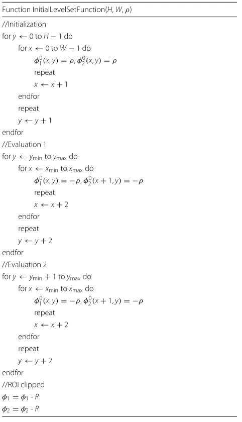
Table 2Definition ofφ0

1(x,y),φ20(x,y)

Function InitialLevelSetFunction(H,W,ρ)

//Initialization fory←0 toH−1 do

forx←0 toW−1 do φ0

1(x,y)=ρ,φ20(x,y)=ρ repeat

x_←x₊1 endfor repeat

y_←y₊1 endfor //Evaluation 1 fory←ymintoymaxdo

forx←xmintoxmaxdo φ0

1(x,y)= −ρ,φ02(x+1,y)= −ρ repeat

x←x+2 endfor repeat

y←y+2 endfor //Evaluation 2

fory_←ymin+1 toymaxdo forx_←xmintoxmaxdo

φ0

1(x,y)= −ρ,φ02(x+1,y)= −ρ repeat

x←x+2 endfor repeat

y←y+2 endfor //ROI clipped φ1=φ1·R

φ2=φ2·R

The pseudo-code for definition of φ0₁(x,y),φ₂0(x,y) is shown in Table 2, where the image dimension isW×H, ρ >0 is a constant with any value, and the ROI is bounded by a rectangle: {(x,y)|xmin≤x≤xmax,ymin≤y≤ymax}.

In this case, the relationship between membership func-tions and level set funcfunc-tions is given by:

⎧ ⎨ ⎩

M1(x)=1−H(φ1(x)) M2(x)=H(φ1(x))H(φ2(x)) M3(x)=H(φ1(x))(1−H(φ2(x)))

(24)

It is worth pointing out that the member functions

mentioned meet 0≤Mi(x)≤1 and

3

i=1

Mi(x)=1.

3.4 ROI-based numerical implementation

In order to remove the influence of noise in the back-ground and reduce computational cost, we propose an ROI-based implementation for the aforementioned algorithm.

In numerical practice, the Dirac functionδ(x)in (12) is smoothed as:

δ(x)= 1

π

2_+x2 (25)

Iteration forφjis proposed by:

φn+1

j =φjn+τ ∂φj

∂t (26)

Table 3Parameters for MRI in this paper

Width 96 Modality MR

Height 192 Repetition time 36 s

Bit depth 12 Echo time 9.2 s

Slice thickness 1 mm Imaging frequency 63.6250

Pixel spacing (1.0417mm, 1.0417mm)

Protocol name COR 3D

Table 4Parameters related to experiments

N η p σ ν μ τ

3 0.7 4 4.0 4.0 1.0 1.0 0.1

In this paper, the window functionKis taken as a Gaus-sian function with a standard deviation σ, denoted by

Kσ. Our proposed ROI-based numerical implementation is presented as follows:

1. ROI mask.I=I·R.

2. Initialization. Set the following parameters:N,η,p, σ,ν,μ,andτ. Initializeb andφ1,. . .,φk. Due to their invariability during iterative procedures, we prepareG,GGT,1∗Kσ,(1∗Kσ)·I2,(G∗Kσ)·I andGGT∗K_σ.

3. Iterative procedure. For thei th iteration, first update cvia (13). Second, updatevia (25), (12), and (26). Finally, updateb via (21), (22), and (23).

4. ROI mask.φj=φj·Rfor next iteration. 5. Redo step (iii) untili exceeds the predefined

maximal iteration.

4 Results and discussion

We analyzed 112 frames of MR brain images; detailed information can be seen in Table 3. The algorithm was implemented using the Microsoft Visual Studio devel-opment platform with the Open CV (Computer Vision) library, and Matlab. In this paper, we have used the same parameters listed in Table 4, except the specific statement. In the experiments, the number for the maximal iteration needed is 50. The energy objective function in (9) keeps descending, shown in Fig. 4. This shows that our proposed method has good convergence.

Fig. 4Energy functional values in the iterations

4.1 Segmentation results

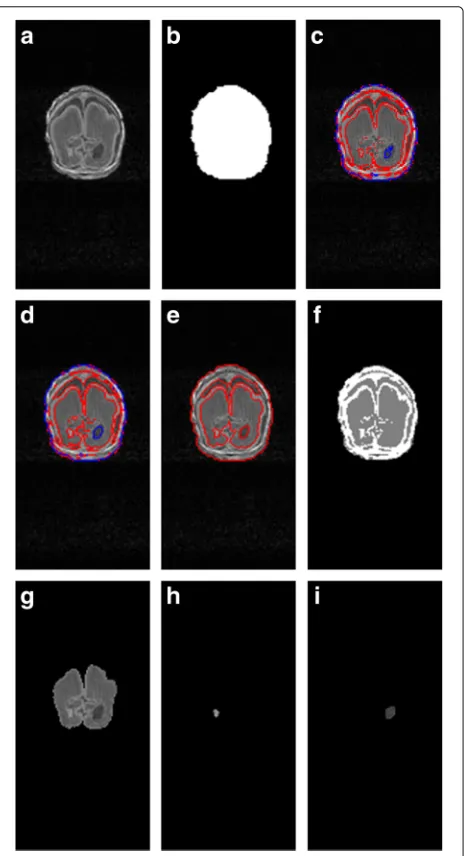
An overview of the proposed method for MRI segmenta-tion is shown in Fig. 5. Here, the original image is shown in Fig. 5a, whose coarse segmentation result, namely ROI, is shown in Fig. 5b. After 10 iterations, the curve evolves as shown in Fig. 5c. After 50 iterations, the final con-tour and segmentation results are illustrated in Fig. 5d–f. Three split parts of segmentation results in Fig. 5g–i demonstrate the capability of our method to segment the bright and dark blobs (high likelihood of potential abnormality) simultaneously. Here, in order to retain the running results by our scripts, contours in red and blue

imply that the boundaries are induced by different level set functions, as mentioned in Section 3.3. Without loss of generality, we henceforth adopt red contours later in this paper.

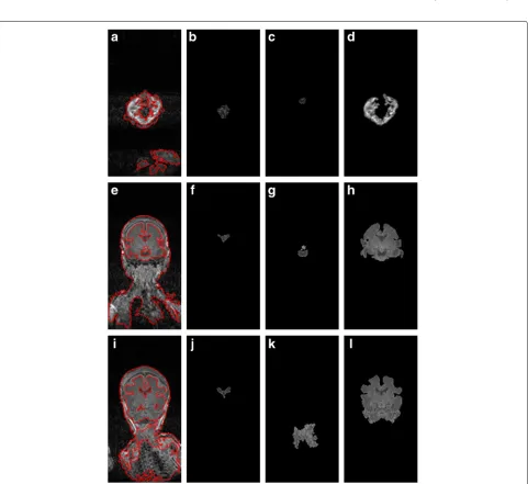
Experimental results for the other frames are shown in Fig. 6. The relevant parameters are employed as shown in Table 4. The segmentation performance verifies that the listed parameters are image independent.

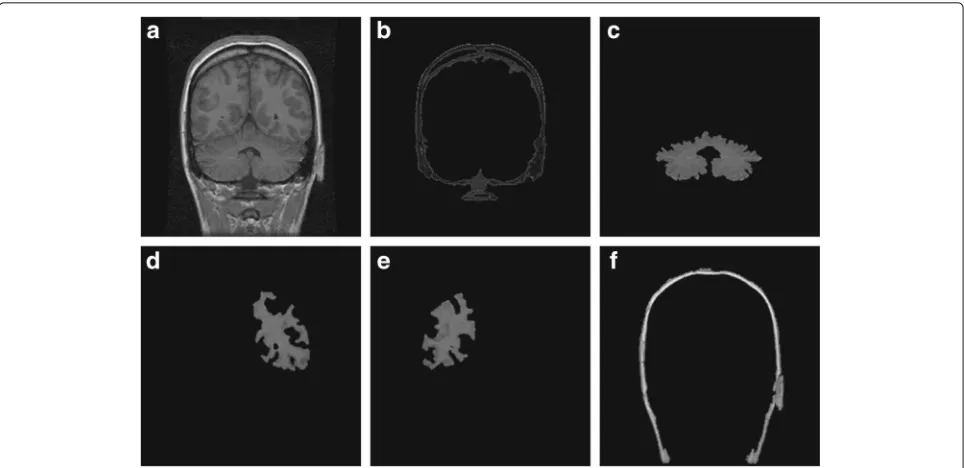
Outside the data set mentioned above, we experi-ment on the MR brain images [38], which includes 60 images (width 256, height 256, bit depth 16). Taking the 6th image (see Fig. 7a) as an example, our pro-posed method can segment the images into parts: skull (see Fig. 7b), white matter (see Fig. 7c, d), and other parts.

4.2 Segmentation assessment

For objective evaluation of our method, we consider man-ual contours drawn by specialists as the ground truth. We introduce two metrics to segmentation assessment. One metric m1is defined to estimate the difference between

the ground truth and the contours extracted by our method. For one specific ground truth contour, we first select its nearest contour edge in contours from our pro-posed method, then we calculate the distance between the contour pair. The other metricm2is to account for how

many accurate possible abnormal blobs are detected. Assuming ground truth contours are denoted by

Cg = Cg1,C2g,. . .,C ng g

!

, and contours from the

pro-posed method are denoted byCp= Cp1,Cp2,. . .,C np p

! .

Fig. 7Segmentation processes for the other frames:athe 14th MR image,b–dsegmented parts,ethe 50th MR image,f–hsegmented parts,ithe 67th MR image, andj–lsegmented parts

For theith contour, the corresponding best matching contour in the proposed method is defined by:

ki=argmin k

⎧ ⎪ ⎨ ⎪ ⎩

pj∈Cgi

d

pj,Cpk

:k=1, 2,. . .,np ⎫ ⎪ ⎬ ⎪ ⎭

whered

pj,Cpk

is the distance from pointpjto contour

edgeCk p.

Therefore, the measurement depicting the difference of the contours representing the ground truth and the proposed method is given by:

m1=

1

ng ng

i=1

⎛ ⎜

⎝

pj∈Ckip

dpj,Cgi ⎞_⎟

⎠/%%%Cki_p%%_% (27)

where%%%Cpki%%%is the number of elements inCpki.

Assuming Np is the number of potential abnormality blobs detected by the proposed method and Ng is the number of possible abnormality blobs provided by spe-cialists, the metricm2is defined by the ratio ofNptoNg:

Table 5Comparison of segmentation metrics

Metrics Li’s method [22] Our method

m1 1.64 0.62

m2 29% 97%

m2 = Np

Ng ×

100% (28)

The smaller m1 or the bigger m2 is, the better the

segmentation result is. Comparison results between Li’s method and our method using these metrics are shown in Table 5 and Fig. 8.

4.3 Comparisons with existing methods

Without less noise affected MRI [39], our and Li’s method [31] give similar contours, shown in Fig. 9, which demon-strates the validity of our method. Our method prevails in

Fig. 9Comparison with the work [31]:aoriginal MR image,bresult via [31], andcresult based on our method

two aspects: (1) the outer contour is more smooth than Li’s method, and (2) it detects more subtle bright or dark blobs which are potential abnormalities.

Compared to bias field estimation [22]-based segmen-tation (see Fig. 10b), our method produces more accurate segmentation result with fine localization of regions of interest, as shown in Fig. 10d. However, result based on [22] cannot give the contour directly and it misses the black blob. Furthermore, it cannot output accurate closed regions, such as the gray matter region (polygon bounded by a closed yellow curve in Fig. 10d). In comparison with our method, traditional level set method [28] only extracts the outermost contours, as shown in Fig 10c. Our method detects complete contours (see Fig. 10d), in which the con-tour is highlighted in yellow, including missed detections in [28].

The authors in [31] take intensity inhomogeneities and level set method into account for image segmen-tation. The difference between ours and the one in [31] lies in that we minimize the w, while the latter

minimizes thebdirectly. Therefore, our method can seg-ment more regions of interest, including bright and dark blobs simultaneously, as shown in Fig. 11, which helps to improve diagnosis in medical applications.

4.4 Discussion

In this paper, we introduced Otsu algorithm to remove background noise from original image. It is simple but effective in coarse segmentation. Such course segmen-tation helps to improve accuracy in final segmensegmen-tation. Additionally, bias field polyfit estimation gives a more continuous bias field map, see Fig. 2b. Furthermore, customized initial level set functions proposed in this paper helps to segment weak-edged, low-resolution MR brain images. In a sense, we incorporate bias field esti-mation into multi-phase level set method to acquire fine segmentation with low computational complexity. The proposed method can outline possible abnormali-ties. However, lesion recognition is to be determined in future work.

Fig. 11Comparison with [31]:athe 84th MR image,bthe result via [31], andcthe result based on our method

5 Conclusions

In this paper, we proposed a robust MRI abnormal-ity detection method, which utilized background noise removal and polyfit level set method. Note that we improve the work in [22, 31], with our method being able to segment subtle bright or dark blobs automatically. Background removal helped us to exclude background noise, which also provided ROI to speed up successive processing. Polyfit level set method with customized ini-tial level set functions in this paper does segment MRIs into individual parts, including tiny tissues. Experimental results demonstrate that our method has good perfor-mance in extracting all the blobs in MRIs, in which, there are potential lesions. But, as for each divided part, whether it is abnormal is yet to be determined. In future work, we will apply our technique on brain injury detection, such as for white matter injury detection.

Acknowledgements

The authors would like to thank NSERC, Canada, for their financial support of this research.

Funding

The work was supported in part by the Open Project of the Artificial Intelligence Key Laboratory of Sichuan Province under grant nos. 2014RZY02 and 2017RZJ03, the Open Project of Sichuan Province University Key Laboratory of Bridge Non-destruction Detecting and Engineering Computing under grant no. 2014QZY01, Natural Science Foundation of Sichuan University of Science and Engineering (SUSE) under grant nos. 2015RC08 and

2017RCL23, and Educational reform project of SUSE under grant no. JG-1707. The work was also supported in part by the Training Programs of Innovation and Entrepreneurship of Sichuan Province for Undergraduates under grant no. 201710622088. The work was also supported in part by Guangxi Key Laboratory of Cryptography and Information Security under grant no. GCIS201607.

Availability of data and materials Not applicable.

Authors’ contributions

CL and AB designed the algorithm, and CL wrote the paper and also performed the experiments. IC and AB reviewed and edited the manuscript. JY gave a critical suggestion on experimental section. All authors read and approved the manuscript.

Ethics approval and consent to participate Not applicable.

Consent for publication Not applicable.

Competing interests

The authors declare that they have no competing interests.

Publisher’s Note

Springer Nature remains neutral with regard to jurisdictional claims in published maps and institutional affiliations.

Author details

1_{Artificial Intelligence Key Laboratory of Sichuan Province, Sichuan Province}

University Key Laboratory of Bridge Non-destruction Detecting and Engineering Computing, Zigong, China.2_{Sichuan University of Science and} Engineering, 643000 Zigong, China.3_{Department of Computing Science,} University of Alberta, T6G 2H1 Edmonton, Canada.4_{Guangxi Key Laboratory of} Cryptography and Information Security, 541004 Guilin, China.

Received: 30 June 2017 Accepted: 22 August 2017

References

1. HM Duvernoy, JL Vannson, P Bourgouin, EA Cabanis, F Cattin, J Guyot, MT Iba-Zizen, P Maeder, B Parratte, L Tatu, et al,The Human Brain: Surface, Three-Dimensional Sectional Anatomy withMRI, and Blood Supply. (Springer, New York, 1999)

2. J Geng, J Xie, Review of 3-D endoscopic surface imaging techniques. IEEE Sensors J.14(4), 945–960 (2014)

3. RW Brown, YCN Cheng, EM Haacke, MR Thompson, R Venkatesan,Magn. Reson. Imaging Phys. Principles Sequence Design. (Wiley, New York, 1999) 4. GT Herman, WN Brouw,Image Reconstruction from Projections—Fundamentals

of Computerized Tomography. (Academic, New York, 1980)

of the heart from CT scans. Eurasip J. Image Video Process.2014(1), 1–13 (2014)

6. Y Ohe, T Hayashi, I Deguchi, T Fukuoka, Y Horiuchi, H Maruyama, Y Kato, H Nagoya, A Uchino, N Tanahashi, MRI abnormality of the pulvinar in patients with status epilepticus. J. Neuroradiol.41(4), 220–226 (2014) 7. I Cheng, SP Miller, EG Duerden, K Sun, V Chau, E Adams, KJ Poskitt,

HM Branson, A Basu, Stochastic process for white matter injury detection in preterm neonates. NeuroImage Clinical.7, 622–630 (2015)

8. U Vovk, F Pernuš, B Likar, A review of methods for correction of intensity inhomogeneity in MRI. IEEE Trans. Med. Imaging.26(3), 405–421 (2007) 9. J Haselgrove, M Prammer, An algorithm for compensation of surface-coil

images for sensitivity of the surface coil. Magn. Reson. Imaging.4(6), 469–472 (1986)

10. DL Thomas, E De Vita, R Deichmann, R Turner, RJ Ordidge, 3D MDEFT imaging of the human brain at 4.7 T with reduced sensitivity to radiofrequency inhomogeneity. Magn. Reson. Med.53(6), 1452–1458 (2005)

11. T Andersson, T Romu, A Karlsson, B Norén, MF Forsgren, Ö Smedby, S Kechagias, S Almer, P Lundberg, M Borga, OD Leinhard, Consistent intensity inhomogeneity correction in water–fat MRI. J. Magn. Reson. Imaging.42(2), 468–476 (2015)

12. A Sharma, R Bammer, VA Stenger, WA Grissom, Low peak power multiband spokes pulses for B1+ inhomogeneity-compensated simultaneous multislice excitation in high field MRI. Magn. Reson. Med. 74(3), 747–755 (2015)

13. W Dominguez-Viqueira, BJ Geraghty, JY Lau, FJ Robb, AP Chen, CH Cunningham, Intensity correction for multichannel hyperpolarized 13_{C imaging of the heart. Magn. Reson. Med.75(2), 859–865 (2015)} 14. T Oida, M Tsuchida, H Takata, T Kobayashi, Actively shielded bias field

tuning coil for optically pumped atomic magnetometer toward ultralow field MRI. IEEE Sensors J.15(3), 1732–1737 (2015)

15. AH Andersen, Z Zhang, MJ Avison, DM Gash, Automated segmentation of multispectral brain MR images. J. Neurosci. Methods.122(1), 13–23 (2002) 16. EB Lewis, NC Fox, Correction of differential intensity inhomogeneity in

longitudinal MR images. Neuroimage.23(1), 75–83 (2004) 17. P Vemuri, EG Kholmovski, DL Parker, BE Chapman, inInformation

Processing in Medical Imaging. Coil sensitivity estimation for optimal SNR reconstruction and intensity inhomogeneity correction in phased array MR imaging (Springer, Berlin, 2005), pp. 603–614

18. J Ashburner, KJ Friston, Unified segmentation. Neuroimage.26(3), 839–851 (2005)

19. A Banerjee, P Maji, inComputer Analysis of Images and Patterns.

Contraharmonic mean based bias field correction in MR images (Springer, Berlin, 2013), pp. 523–530

20. SK Adhikari, JK Sing, DK Basu, M Nasipuri, PK Saha, A nonparametric method for intensity inhomogeneity correction in MRI brain images by fusion of Gaussian surfaces. Signal Image Video Process.9(8), 1945–1954 (2015)

21. W-Q Deng, X-M Li, X Gao, C-M Zhang, A modified fuzzy C-means algorithm for brain MR image segmentation and bias field correction. J. Comput. Sci. Technol.31(3), 501–511 (2016)

22. C Li, JC Gore, C Davatzikos, Multiplicative intrinsic component optimization (MICO) for MRI bias field estimation and tissue segmentation. Magn. Reson. Imaging.32(7), 913–923 (2014) 23. T Xu, I Cheng, R Long, A Mandal, Novel coarse-to-fine dual scale

technique for tuberculosis cavity detection in chest radiographs. Eurasip J. Image Video Process.2013(1), 1–18 (2013)

24. DL Pham, C Xu, JL Prince, Current methods in medical image segmentation. Annu. Rev. Biomed. Eng.2(1), 315–337 (2000) 25. H Narkhede, Review of image segmentation techniques. Int. J. Sci.

Modern Eng.1(8), 54–61 (2013)

26. J Duan, Z Pan, X Yin, W Wei, G Wang, Some fast projection methods based on Chan-Vese model for image segmentation. Eurasip J. Image Video Process.2014(1), 1–16 (2014)

27. R Malladi, JA Sethian, BC Vemuri, Shape modeling with front propagation: a level set approach. IEEE Trans. Pattern Anal. Mach. Intell.17(2), 158–175 (1995)

28. C Li, C Xu, C Gui, MD Fox, inIEEE Computer Society Conference on Computer Vision and Pattern Recognition (CVPR). Level set evolution without re-initialization: a new variational formulation (IEEE, California, 2005), pp. 430–436

29. G Zhu, S Zhang, Q Zeng, C Wang, Boundary-based image segmentation using binary level set method. Opt. Eng.46(5), 050501–3 (2007) 30. C Li, C Xu, C Gui, MD Fox, Distance regularized level set evolution and its

application to image segmentation. IEEE Trans. Image Process.19(12), 3243–3254 (2010)

31. C Li, R Huang, Z Ding, JC Gatenby, DN Metaxas, JC Gore, A level set method for image segmentation in the presence of intensity inhomogeneities with application to MRI. IEEE Trans. Image Process. 20(7), 2007–2016 (2011)

32. A Dirami, K Hammouche, M Diaf, P Siarry, Fast multilevel thresholding for image segmentation through a multiphase level set method. Signal Process.93(1), 139–153 (2013)

33. MT El-Melegy, HM Mokhtar, Tumor segmentation in brain MRI using a fuzzy approach with class center priors. Eurasip J. Image Video Process. 2014(1), 1–14 (2014)

34. CG Koay, PJ Basser, Analytically exact correction scheme for signal extraction from noisy magnitude MR signals. J. Magn. Reson.179(2), 317–322 (2006)

35. S Aja-Fernández, C Alberola-López, C-F Westin, Noise and signal estimation in magnitude MRI and Rician distributed images: a LMMSE approach. IEEE Trans. Image Process.17(8), 1383–1398 (2008) 36. N Otsu, A threshold selection method from gray-level histograms. IEEE

Trans. Syst. Man Cybernet.9(1), 62–66 (1979)

37. AA Aboaba, S Hammed, OO Khalifa, AH Abdalla, Region and active contour-based segmentation technique for medical and weak-edged images. J. Comput. Appl. Math.1(3), 72–78 (2015)

38. MATLAB Central (2017). https://www.mathworks.com/matlabcentral/ mlc-downloads/downloads/submissions/4879/versions/7/download/ zip/MRI_Brain_Scan.zip. Accessed 01 Feb 2017