ORIGINAL PAPER
An activity-based system of models for student mobility
simulation
Gabriella Mazzulla
Received: 4 November 2008 / Accepted: 16 October 2009 / Published online: 4 November 2009 #European Conference of Transport Research Institutes (ECTRI) 2009
Abstract
Purpose The objective of this paper is to provide a tool for transport system planning. Therefore, a system of models for student mobility simulation on a university campus is proposed.
Methods An activity-based approach has been adopted. The system of models is sequential, in which each choice dimension is linked to the previous one and involves the choices made at a lower level, and it is made up of multinomial and hierarchical Logit models. Additionally, the Revealed and Stated preferences technique has been adopted for investigating user choice behaviour in the hypothesis that an innovative transport system is realized to access the campus.
ConclusionsThe proposed system of models adopt the activity-based travel approach combined with the conjoint use of the RP and SP methodologies, allowing a better understanding and prediction of users responses to travel demand management measures. The model structure is very realistic for student mobility simulation, helping the analyst in evaluating the effects of park pricing policies and the introduction of a new transport system in the travel users choices.
Keywords Activity-based . System of models Revealed and stated preferences
1 Theoretical framework
Over the last 30 years, considerable advances in travel demand modelling have been made and, particularly, in discrete choice analysis. The trip-based approach has been widely studied and applied [6,17,34]. Afterwards, the tour-based approach has allowed some complexities to be addressed, such as trip-chaining and interrelations among travel from home to one or more activity locations and back home again. Frequently, these models assume that each tour has a primary destination in which the main activity is carried out; this activity is the major motivation for the journey. Tour-based models have been developed since 1980 in the Netherlands [14,21–23]. Some system of models have been estimated and applied in the US [33, 36], in Sweden [2], in Germany [35], and in Italy [13]. Systems of more advanced models simulate the travel-pattern and analyze every tour in one or more day, by taking into account the existing conditionings among the tours made by people in a day or a week; in some cases, also the tours realized by the other family members are taken into account [1,5].
As is well-known, mobility demand is derived from the need to conduct several activities in different places. Activities and trips have cause and effect relationship. Therefore, since the early seventies and more markedly about 10 years later, many authors have preferred an innovative approach, known in the literature as activity-based, because it is based on the activities rather than on the trip analysis. For this reason, the activity-based models can be defined as activity participation models.
According to the activity-based approach, the mobility demand is simulated by taking into account the relationship between activities and trips and the spatio-temporal constraints in which people make activity and travel decisions. Adler and Ben-Akiva first introduced the activity G. Mazzulla (*)
Department of Land Use Planning, University of Calabria, Via Pietro Bucci, cubo 46/B,
duration and activity scheduling concepts [1], while Bowman and Ben-Akiva presented the first full-day model which integrates the activity participation decision for all activities and travels spanning a day, including the dimensions of destinations, modes and timing of the derived travel [9]. The activity-based travel theory has been widely discussed in the literature; significant reviews were provided by Damm [15], Golob and Golob [20], Pas [30], Kitamura [26], Jones [25], Axhausen and Garling [4], Ettema and Timmermans [18]. An historical development of the activity-based models has been recently proposed by Bowman [8]. The state of the art of the activity-based models is continuously in advance, and several systems of models have been developed in academic setting by Hensher and Ton [24], Arentze and Timmermans [3], Pendyala et al. [32], and many other authors.
In the last twenty years modellers have attempted to incorporate the activity-based theory into travel forecasting models. Very promising results have been enabled by the advance of computing technology. Operational systems were implemented for the urban travel demand forecasting in several city, particularly in the US (such as San Francisco, Sacramento, New York, Dallas, Columbus and so on), as well as for the regional travel demand forecasting in the city of Sacramento (California) [12]. Systems of models were used also for testing parking policy interventions, as an example for the city of Truro (Cornwall) [16].
During the past few years the activity-based travel theory has been combined with the conjoint use of the RP and SP methodologies, even if there are still few proposed applica-tions; as an example one could refer to Shiftan et al. [37].
Traditionally, mobility surveys are effected by the RP method, related to the actual travel behaviour of the users in a real context. Since the early 1970s, some marketing researchers have devised new survey method-ologies, known in the literature as Stated Preferences techniques (SP); also transport researchers immediately showed some interest in these techniques; the first applications in this field began in the early eighties. The SP techniques are methodologies based on the statements of the interviewed about their preferences in different choice contexts, real, hypothetical or experi-mental. Therefore, an important innovation was intro-duced: the possibility of considering choice alternatives unavailable at the time of the surveys [31].
SP survey methodologies involve the definition of the choice alternatives, of the attributes (or factors) consid-ered for each alternative, of the levels of variation of each attribute, of the choice contexts (scenarios) pro-posed to the decision-makers, of the type of preference asked, of the modality of interview management [27,29]. The number of possible scenarios depends on the combinations among the alternatives, the attributes and
the levels of each attribute. The analyst’s aim is to establish the relative effect of each attribute on the overall utility associated with each option by the individuals.
The SP data applications related to stated choices in a specific hypothetical context have assumed a growing impor-tance in the last few decades. Some authors have proposed methodologies for using this kind of data, and models derived from them [28, 31]. However, many authors assert that a direct application of these models in order to forecast the choices made by the users is not very appropriated [11,19]; as a consequence, some authors have proposed joint calibration models using RP and SP data (see, for example, [7]).
In the case of joint calibration using RP and SP data, the scaling estimation methodology is usually applied; this methodology allows variability among different types of data jointly used in a statistic analysis to be considered. The joint estimation of the model parameters can be obtained by maximizing the Likelihood function of the joined sample, with the hypothesis that the two samples are independent. The function is non-linear because the scale factor multi-plies not only the attributes, but also the parameters of the SP utility function. For this reason, the estimation proce-dure of the scale factor is an operational research problem, which can be resolved through a specific software able to manage non-linear Likelihood functions directly, or through techniques allowing the use of non-specific software developed for the discrete choices analysis. In this last case, three methods are reported in the literature: the first one, proposed by Ben-Akiva and Morikawa [7], based on a sequential estimation procedure; the second one, proposed by Bradley and Daly [10], based on the simultaneous estimation of the RP/SP model parameters and the scale parameter; the third one, proposed by Swait and Louviere [38], based on an iterative estimation procedure.
In this paper an original formulation of a system of random utility models is introduced. The user decisional process is simulated according to a sequential approach, or rather through a set of linked sub-models reproducing the different choice dimensions for consecutive stages. An activity-based approach has been adopted. In the proposed system, some user choice dimensions and, specifically, the transport mode choice, is modelled by using both RP and SP data. The conjoint use of such data allows the analysis and the simulation of both current and future consumer behaviour in real scenarios, but also in hypothetical scenarios, with the aim of considering non-existing transport modes among the choice alternatives.
some calibration results are proposed in order to verify the validity of the system. The calibration was effected by means of a survey carried out on the students of an Italian university campus in the autumn of 2004. A brief conclusive section is reported at the end of the paper.
2 Experimental context
An experimental survey was realized on the campus of the University of Calabria, situated in the urban area of Cosenza (in the South of Italy). The campus is attended by 32,000 students and 2,000 members of staff approximately (November 2004). Currently the University is served by a bus service, which does not resolve the problem of student mobility demand in a suitable way; where possible, students prefer to use individual transport, producing congestion both on the access and on the internal campus road networks. The survey, realized in the autumn of 2004, involved a sample of 1,477 students, with a sampling rate equal to 4.5% approximately. These students partly live with their family (780 students, whose 405 in the urban area) and partly live with other students, “lodged” by the campus administration (697 students, whose 690 in the urban area). The inter-viewed students are equally divided between “inside” (43%) and“outside”(57%) students; the“outside”students are people living in a place distant from the campus more than an hour. The sample is divided, also, in“in course”and “out course”students; in Italy, the“out course”condition relates to a university student who has not finished his studies in the prescribed time. The“in course”students are 72% of the total. 90% of the sample is between 18 and 25 years old; most of this are younger than 21. They primarily belong to a middle class of family income (45% of the total), or lower-middle (19%), or upper-middle (19%).
The students described activity and trip sequences in the tours made in a day. The tours are the trip sequences with the first origin and last destination at home (home-based tours), and with one or more sojourns on the campus. Each activity is characterized by the typology and duration, and each trip is defined by origin, destination, duration and transport mode used. In total, the students made 1,631 tours with at least one stop in the university area; 1,323 students made only one tour in a day; 154 students made two tours. As expected, most of the tours were realized for carrying out didactic activities; in 66% of the cases for attending a lesson, in 14% of the cases for conducting other study activities and in 13% of the cases for effecting a different didactic activity from the first ones. However, other activities like handling of personal business or recreation/relational activities were undertaken in the tours but were not considered as primary activities. About 64% of the tours
were trip-tour (i.e. with a single outward and one return trip); the remaining 36% were tours made up of three or more trips (trip-chain), in which two or more activities were combined.
Additionally, the survey was planned to collect RP and SP data on the same sample. The RP survey was done in order to collect some students’socio-economic character-istics and information regarding transport mode actually used to reach the university campus. An SP experiment was designed in order to estimate a strategy for increasing the use of public transport services connecting the urban area to the campus; the strategy consists in conjugating policies for the improvement of the public transport services with demand management policies, i.e. car-park pricing. A new transport system connecting the urban area with the campus was proposed; this system is characterized by a high frequency and a low travel time. At the same time, park pricing policies in the university area were adopted. The access trip was equally realized with a private (45%) or a public transport mode (46%); other transport modes were not much used. Most of the Engineering students realized the access trip by car (72%).
In the SP experiment, the users expressed their degree of preference (according to a semantic scale from 1 to 5) about 7 hypothetical choice scenarios; each scenario includes both car and bus alternatives. The car alternative is characterized by a parking cost attribute, varying from the actual level (free) to an intermediate and high level; the bus alternative is characterized by frequency (low and high) and travel time attributes (equal or lower than the actual time). The results show that the users of the transport system are inclined to accept the policies of mobility management proposed when the use of the car is strongly discouraged through car-park pricing policies. In fact, the improvement of the public transport services involves a meaningful variation in the modal split when an incisive additional cost is imposed on the individual use of the car.
3 The proposed system of models
3.1 General structure
activity in the university area; in the second one the students undertake several activities in the same tour, some inside the campus and other outside the campus, or in the urban area of Cosenza. No hypotheses were made about the connection among the tours realized by the same student in a day. Only the “first tour” was analyzed and simulated because of the low percentage of students which have made more than one tour in a day (12%). This circumstance could represent a limitation of the analysis.
Each simulated tour is characterized by a predominant activity producing the need to make the tour, named primary activity PA. For defining the primary activity of each tour, a hierarchy of activities was formalized, as a function of the spatial and temporal constraints that each activity has in the organization of the same tour. Specifically, the place in which the activity is carried out, the activity type and the chronological sequence were taken into account. It is supposed that the primary activity in the tour is made inside the campus, and each activity effected outside the university area is secondary. A hierarchy of the activity was defined among the activities carried out inside the campus, according to the following order: attending a lesson; other didactic or study activities; meal; handling personal business; recre-ation and/or relrecre-ational activity. If two activities of the same hierarchical level are made in a tour, the primary activity is the first in a chronological order.
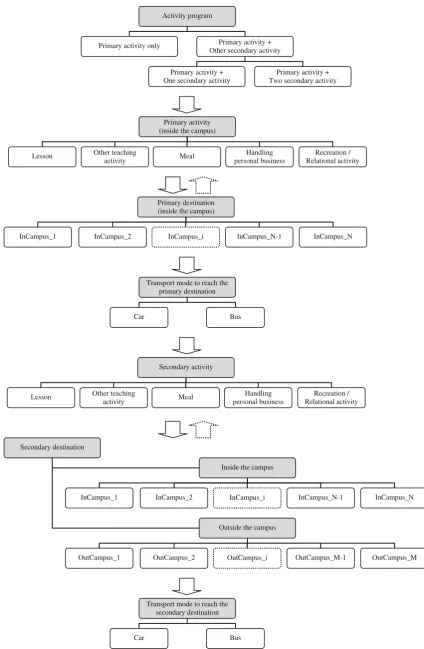
The proposed system of models simulates the user decisional process in six choice dimensions, each included in a different sub-model, whose sequence is introduced in the flow chart shown in Fig. 1. The higher hierarchical level is represented by the activity program choice model AP. The next hierarchical level is repre-sented by the models related to the primary activity, and specifically: choice of the primary activity PA, choice of the primary destination PD, in which this activity is carried out, and choice of the transport mode MPD used to
reach this destination from home. Equally, a set of models relates to the possible secondary activities SA in the tour, and specifically: choice of the secondary activity SA, choice of the secondary destination SD, in which this activity is effected, and choice of the transport mode MSD used for reaching this destination.
The adopted sequential approach involves that the choices referred to a certain choice dimension are conditioned by the choices simulated through the sub-model at the upper level. In two cases the choices simulated by a certain sub-model also condition the choices simulated by the upper sub-model. This is shown in Fig. 1 by a discontinuous line of connecting arrows among the different models. In analytical terms, this reciprocal conditioning is represented by a specific variable introduced in the utility function of the alternatives of the model at the upper level, which considers the choices also made by the users at the lower level. Specifically, this link is introduced between the models for choosing the type and place of the activity, and the destination choice model, in reference to both the primary and secondary activities.
The structure of the system of models indicates the sequence in which the choices on each dimension are made by the users, and choice reciprocal influence. The order of the sequence with which the sub-models are introduced could be different from the one described. For instance, the choice related to the activity program could be made after the choice of the primary activity in the tour, because the user chooses to make a possible secondary activity as a function of the spatio-temporal constraints related to the primary activity.
The order of the sequence is usually verified in the model calibration phase, verifying the different hypotheses by statistical tests performed on the single parameters and sub-models. Nevertheless, in this case, the verification was not effected.
The sequence of the sub-models introduced in Fig.1can be expressed, in analytical terms, by the following formula:
p APð ;PA;PD;MPD;SA;SD;MSD=TÞ ¼p APð =TÞ p PAð =T;APÞ
p PDð =T;AP;PAÞ
p MPDð =T;AP;PA;PDÞ
p SAð =T;AP;PA;PD;MPDÞ
p SDð =T;AP;PA;PD;MPD;SAÞ
p MSDð =T;AP;PA;PD;MPD;SA;SDÞ
ð1Þ
Symbols in formula (1) have the following meaning:
p(AP,PA,PD,MPD,SA,SD,MSD/T) represents the proba-bility that the student, considered that he had decided to go from home to the campus and therefore to make the
OutCampus_2
Outside the campus
OutCampus_i OutCampus_M-1
OutCampus_1 OutCampus_M
InCampus_2
Inside the campus
InCampus_i InCampus_N-1
InCampus_1 InCampus_N
Secondary destination
Primary activity only Primary activity + Other secondary activity Activity program
Primary activity + One secondary activity
Primary activity + Two secondary activity
Lesson Other teaching activity
Primary activity (inside the campus)
Meal Handling personal business
Recreation / Relational activity
InCampus_2
Primary destination (inside the campus)
InCampus_i InCampus_N-1
InCampus_1 InCampus_N
Car Bus
Transport mode to reach the primary destination
Lesson Other teaching activity
Secondary activity
Meal Handling personal business
Recreation / Relational activity
Car Bus
Transport mode to reach the secondary destination
p(AP/T)represents the probability, calculated through the activity program choice model, that the student chooses to combine or not the primary activity with one or more secondary activities, assuming that the tour T is known;
p(PA/T,AP) represents the probability that the student, after he has chosen the activity program AP, undertakes the primary activity PA in the campus, assuming that the tour T is known;
p(PD/T,AP,PA)represents the probability that the student, after he has chosen the activity program AP, undertakes the primary activity PA in the primary destination PD inside the campus, assuming that the tour T is known;
p(MPD/T,AP,PA,PD)represents the probability that the student, after he has chosen the activity program AP, uses the transport mode MPD to reach the primary destination PD, where he makes the primary activity PA, assuming that the tour T is known;
p(SA/T,AP,PA,PD,MPD) represents the probability that the student, after he has chosen the activity program AP, undertakes the secondary activity SA combined with the primary activity PA, made in the primary destination PD, reached by the transport mode MPD, assuming that the tour T is known;
p(SD/T,AP,PA,PD,MPD,SA) represents the probability that the student, after he has chosen the activity program AP, undertakes the secondary activity SA, made in the secondary destination SD, inside or outside the campus, combined with the primary activity PA, made in the primary destination PD, reached by the transport mode MPD, assuming that the tour T is known;
p(MSD/T,AP,PA,PD,MPD,SA,SD) represents the proba-bility that the student, after he has chosen the activity program AP, undertakes the secondary activity SA, made in the secondary destination SD, reached by the transport mode MSD, combined with the primary activity PA, made in the primary destination PD, reached by the transport mode MPD, assuming that the tour T is known.
In the proposed system of models the generative phase of the tour was not simulated because the survey was conducted “at the destination”, i.e. each student was interviewed in the place in which he had undertaken his activity.
The proposed system is made up of behavioural models based on random utility theory, with multinomial or hierar-chical Logit structures according to the degree of similarity perceived by the user among the different alternatives.
3.2 Activity program choice model
The first choice dimension simulated by the proposed system of models relates to the activity program; the proposed model is a hierarchical Logit model (Fig. 1), in which the alternatives at the higher level are: to undertake the primary activity PA in a tour only or to associate other secondary activities SA with the primary activity. If the student has chosen to make some secondary activities in his tour, he can subsequently choose to make one or two secondary activities.
The systematic utility functions of each alternative are brought in the expression (2):
VPA¼bBeginT*BeginTþbOtherT*OtherT
VPAþ1SA¼bPADur*PADurþbPAType*PAType
VPAþ2SA¼bTTime*TTimeþbModeI*ModeIþbPADur*PADurþbPAType*PAType
ð2Þ
in which:BeginTrepresents a cardinal variable indicating the time of tour beginning;OtherTrepresents the number of other tours realized by the user in the same day (cardinal variable); PADur represents a cardinal variable indicating the duration of the primary activity; PAType
represents a dummy variable with value equal to 1 or 0 depending on the primary activity, which can be“to attend a lesson” or other activities; TTime represents the total time from home to the primary destination in the campus;
ModeIrepresents a dummy variable with value equal to 1 or 0 depending on the transport mode used for reaching the first destination in the university area, which can be individual or not.
The variables introduced in the different systematic utility functions explain the temporal constraint which the user has to
take into account in order to program his tour and the existing interactions between this tour and the activity program.
3.3 Primary activity choice model
The proposed model has a multinomial Logit structure. The systematic utilities of the choice alternatives are expressed as a function of socio-economic indicators, such as the student’s “inside” or “outside” condition or the student’s “in course” or “out course” condition. Other indicators relate to the temporal constraints taking into account the interactions between the activity program and travel program, such as the hour of the tour beginning.
In addition, an inclusive variable (LogSum) is used in order to take into account the choices which the students can make among the zones in which the activities are placed. The basic hypothesis is that the spatial distribution of the activities can play a key role in the choice of the primary activity; so, the utility related to the various primary activities (PA) can be expressed as a function of the utility related to the various zones in which these activities can be made. The LogSum variable represents the expected value of the maximum utility perceived by the student for choosing a destination zone (PD), and assumes the following expression:
LogSum PAð Þ ¼ln X pd2PD
exp½V PAð ;PDÞ ð3Þ
The systematic utility functions of each choice alterna-tive are expressed through the formula (4):
VLesson¼bStCourseStCourseþbLogSumLogSum PAð Þ
VODidAct¼bLogSumLogSum PAð Þ
VMeal ¼bOutSideOutSideþbLogSumLogSum PAð Þ
VHoldPerAff ¼bCoursesCoursesþbLogSumLogSum PAð Þ
VRecrAct ¼bHBeginT HBeginTþbLogSumLogSum PAð Þ ð4Þ
in which:StCourserepresents a dummy variable with value equal to 1 or 0 depending on the student’s “in course”or “out course” condition; OutSide represents a dummy variable with value equal to 1 or 0 depending on the student’s “inside” or “outside” condition; LogSum(PA)
represents the expected maximum utility related to the choice of the primary destination PD;Coursesrepresents a dummy variable with value equal to 1 or 0 depending whether the courses are active in the period of surveys or not;HBeginTrepresents a dummy variable with value equal to 1 or 0 depending on the hour of the tour beginning (during the morning or in the afternoon).
3.4 Primary destination choice model
A multinomial Logit model is proposed for simulating the choice of the place where the student makes the primary activity. As an example, N alternatives are considered, and
the university area in N homogeneous traffic zones is separated (Fig.1).
The utility function of the j-th traffic zone is expressed by the following formula (5):
VInCampus j¼ X
i
bAttriAttr
i
InCampus jþbTTimeTTimeþbModeIModeI
ð5Þ
in which AttrInCampus_ j represents the attractive power, or availability of human resources, of the j-th traffic zone. The
Attrvariable of each zone is different according to the type of the primary activity undertaken in it. Specifically, if the primary activity effected by the student is to attend a lesson, the variable of zone availability is equal to the number of teaching staff; if the primary activity undertaken by the student is a different didactic activity, the variable is equal to the number of technical staff; if the primary activity conducted by the student is to consume a meal, the variable is equal to the number of employees in the cafeteria and the number of restaurants and cafés; if the primary activity undertaken by the student is to settle some personal business, the variable is equal to the number of the administrative staff; if the primary activity effected by student is recreational or relational, the variable is equal to the number of students in the campus and the number of cultural and recreational associations inside the zone.
TheTTimevariable represents the total time from home to the primary destination in the campus; the ModeI
variable represents a dummy variable with value equal to one or zero depending on the transport mode used.
3.5 Transport mode choice model to reach the primary destination
The choice dimension of the transport mode used by the student to reach the primary destination (PD) is simulated through a conjoint RP/SP model; this model was calibrated by using RP data (related to real choice scenarios) and SP data (related to hypothetical choice scenarios). The infor-mation obtained by the SP experiment relate to two possible transport modes, car and bus, which the user can use to reach the primary destination on the campus from home. Therefore, only the students undertaking the primary activity in the first destination on the campus are considered for the calibration of the transport mode choice model to reach the primary destination.
transport), and attributes related to the temporal constraints (number of trips in the tour) have been added. Specifically,
the formula (13) represents the analytical expressions of the systematic utilities of the two considered alternatives:
VCarRP=SP¼bTTimeTTimeþbTCostTCostþbIncomeIncome
VBusRP=SP¼bTTimeTTimeþbTCostTCostþbSexSexþbOutSideOutSideþ
þbNTripsNTripsþbFreqBusFreqBus
ð6Þ
in which: TTime attribute represents the total time from home to the primary destination in the campus, for car and bus alternatives; TCost attribute represents the total cost supported by the user from home to the primary destination on the campus, for car and bus alternatives; Income
attribute indicates the family user income, with a cardinal number that changes from low to high income level; Sex
represents a dummy variable indicating the user gender, which can take a value equal to one for a gender and zero otherwise;OutSiderepresents a dummy variable indicating the student’s “outside” condition, which can take a value equal to 1 if the student is resident in a place distant from the university campus and 0 otherwise; NTrips attribute represents the number of trips in the tour; FreqBus
represents a dichotomous variable which can take a value equal to 1 for high frequency and 0 otherwise.
3.6 Secondary activity choice model
As previously specified, when the students choose their activity program, they can decide to undertake the primary activity only during the tour or to associate with this other, so-called, secondary activities. In the latter case, the system proposes a further choice dimension related to the secondary activity (Fig.1).
The primary activity in the tour is carried out in the university area. The same restriction does not occur, instead, for the secondary activity, so the place of destination can be both on or outside the campus.
The proposed model is also a multinomial Logit, with the same alternatives considered for the primary activity choice model. However, in this case each choice alternative indicates an activity which can be made both in the campus and in urban area of Cosenza.
The systematic utilities of the choice alternatives have the same expressions brought in the formula (4), and the
LogSum variable, in this case, relates to the choice of the secondary destination (SD).
3.7 Secondary destination choice model
If the student chooses to carry out a secondary activity on his tour, the system of models simulates, after the choice of the type of activity, the place in which the same one can be undertaken. For simulating the choice dimension related to the secondary activity spatial distribution, a hierarchical Logit model is proposed, in which there are two alternatives at the higher hierarchical level: the secondary activity carried out inside the university area, the secondary activity undertaken outside the university area (Fig. 1). On the lower hierarchical level are located the traffic zones in which the campus and urban area have been separated. As a rough guide, the university area has been separated in N traffic zones, while the urban area in M traffic zones. Further zones could be considered outside the urban area.
The systematic utilities for the different traffic zones are expressed as a function of an indicator of availability, varying according to the secondary activity and place in which is made, inside or outside the campus. Specifically, as indicators of availability for the inside zones the same variable considered in the primary destination choice model are used, while for the outside zones some additional variables are defined. In particular, if the secondary activity effected outside the campus is to study with other students, the indicator is represented by the number of university students living in the zone; if the secondary activity is entertainment, accompaniment of person or personal busi-ness, the indicator is represented by the number of employees in the private and public services in the zone.
The general expression of the systematic utility functions for the different zones, inside and outside the campus, is (7):
VInCampus j¼
X
i
bAttriAttr i
InCampus jþbTTimeTTimeþbModeIModeI
VOutCampus j¼
X
i
bAttriAttr i
OutCampus jþbTTimeTTimeþbModeI ModeI
ð7Þ
TheTTimevariable represents the total time from home to the secondary destination inside the campus or outside the
3.8 Transport mode choice model to reach the secondary destination
The choice dimension of the transport mode used by the student to reach the secondary destination (SD) is also simulated through a conjoint RP/SP multinomial Logit model, in which the choice alternatives are car and bus, in the two different contexts (Fig.1). The transport mode proposed in the SP context refers to the access trip to the university area from home. For this model, therefore, the sample is represented by the students that carried out a secondary activity at the first destination on the campus.
The model structure can be the same as specified for the choice model of transport mode used for reaching the primary destination (cf formula 6). The variables consid-ered have the same meaning as previously shown.
4 Experimental results
The proposed system of models was calibrated by using the data of a sample of University of Calabria students. The results obtained are satisfactory and the statistical tests show that the experimental data are well replied. Addition-ally, the attribute coefficients of the considered systematic utilities show a good statistical significance.
As a rough guide, the university area was separated in three traffic zones, while the urban area was separated in five traffic zones. Further zones could be considered on or outside the campus. As an example, the results obtained for the activity program choice model and the choice model of the transport mode used for reaching the primary destination are reported. The calibration was made by considering the tour realized by the students living in the urban area (1,243 tours) and, specifically, the “first tours” only (1,095 tours).
4.1 Activity program choice model
In this model the systematic utilities are expressed as a function of the variables representing the temporal constraints and the interaction between the activity and travel program. The variables representing the temporal constraints (PADur, BeginT, and TTime) are expressed in minutes; the variableOtherTis equal to 1 if the student make other tours in the same day and 0 otherwise; the variableModeIis equal to 1 for the private transport mode and 0 otherwise; the variable PAType is equal to 1 if the primary activity is“to attend a lesson” and 0 otherwise.
These variables were inserted in the systematic utility functions of the different alternatives in a linear form, as reported in the expression (2). The calibration was made by
excluding a tour with more than three activities (1,018 tours only in the sample). The obtained calibration results are reported in Table 1.
From the results, it is deduced that all the estimated coefficients have a sign consistent with the meaning of the corresponding variable. Specifically, the coefficient of the BeginT variable has a positive sign, because the student who encounters tour delays is more inclined to realize only the primary activity, for an obvious time constraint. Also the coefficient of theOtherTvariable has a positive sign, because the student who makes more tours during the day is often interested in carrying out one activity only in each tour. This variable has a coefficient higher than the others. The coefficient of the PAType
variable has a positive sign, that is, if the primary activity is “to attend a lesson”then other secondary activities are carried out in the tour. By the positive sign of the coefficient of theTTime variable it is deduced that if the trip time spent for reaching the primary destination is higher, the student is more inclined to realize a complex tour (such as trip-chaining). Also theModeIvariable has a positive sign, indicating that the use of a private transport mode to reach the primary destination induces to realize a more complex tour. Finally, by the assumed negative sign of the coefficient of PADur variable, it is deduced that increasing duration of the primary activity involves an increase of the probability of taking a trip-tour.
All the estimated coefficients are statistically different from zero, at a good level of significance (5%), except the ModeI and PAType. The Likelihood Ratio test indicating the goodness-of-fit of the model is good. The ρ2
and the %RIGHT tests are equal to 0.30 and 70.24% respectively. The expected maximum utility parameter is equal to 1.402.
Table 1 Calibration results of the activity program choice models
Alternative Variables Estimated coefficient t-Student
PA BeginT βBeginT 0.003 4.538
OtherT βOtherT 2.223 6.519 PA + 1SA PADur βPADur −0.002 −3.421
PAType βPAType 0.304 1.889
PA + 2SA TTime βTTime 0.008 2.452
ModeI βModeI 0.123 0.952
PADur βPADur −0.002 −3.421
PAType βPAType 0.304 1.889
θ 1.402 (0.859)
LogL(β) −777.206 LogL(0) −1,118.39
LR 682.363 (χ2with 7 dof: 14.067) r2
0.2988
4.2 Transport mode choice model to reach the primary destination
The transport mode choice models were calibrated on the basis of the student’s choices about their access trip to the university area. The calibrated models are distinguished in the RP model, based on the choices made by the users exclusively in the real context, and in the SP model, based on the choices stated in the hypothetical contexts, by considering as“choice” the alternative to which the users associate, in the rating experiment, a greater degree of preference. Additionally, a conjoint RP/SP model was calibrated.
For calibrating these models (formula6),TTimeattribute is expressed in minutes and TCost attribute in Euros; the cost attribute represents, for the car alternative, the kilo-metric cost valued for the access trip added to the possible cost for car-parking, and the total ticket cost for the bus alternative. The bus frequency is expressed as a dichoto-mous variable with a value equal to 1 for higher frequency and 0 otherwise; this variable is considered in the SP context only. The income attribute varies from 1, for low income, to 5, for high income; the attribute indicating the user’s gender is assumed as a dichotomous variable, equal to 1 for females and 0 otherwise; the variable indicating the student’s “outside”condition has a value equal to 1 when the student is resident in a place distant from the university campus and 0 otherwise.
The results of the estimations and the statistical test are reported in Table 2. For calibrating the conjoint RP/SP model, an iterative estimation method proposed by Swait and Louviere has been applied [38].
The results show that all parameters have a correct sign and a value statistically different from zero, at a good level of significance, except the “sex”variable in the SP model. As expected, the cost and time attribute coefficients have a negative sign, while the bus frequency has a positive sign. Additionally, the“income”and“outside”parameters have a positive sign, as expected for the defined value of the variables.
All the models verify the statistical tests on the goodness-of-fit. The r2 statistics has the maximum value in the RP model (equal to 0.1839), confirming the greater predictive capability of the model, which simulates the choices made in a real context; the conjoint model, instead, allows improve-ment of the predictive capability to the SP model (the r2 statistics is equal to 0.1212 for RP/SP model and 0.1199 for SP model, respectively). The estimation of the monetary value of time (VOT) is different in the proposed models; specifically, in the RP model the VOT is equal to 3.78€/h, indicating that the user is willing to pay this fee in order to save one hour of time, while VOT is much lower in the SP and RP/SP models, assuming a value equal to 0.94€/h and 0.67 €/h, respectively. The strong differences among VOT values can be explained by considering that the parameter related toTTimeattribute has a comparable value for all the three models; vice versa, the parameter related to TCost
attribute has very different values: the value of β2 in SP model is about three times higher than the value in the RP model, and the value in RP/SP model is more than four times higher than the value parameter in the RP model. There is every indication that the choices made by the students in the RP context, which is characterised by free parking, scantly
Table 2 Results of model calibrations
Alternative Variable Parameters RP model SP model RP/SP model
Value estimated t-Student Value estimate t-Student Value estimated t-Student
CAR TTime β1 −0.0138 −2.07 −0.0104 −4.13 −0.0104 −2.68
TCost β2 −0.2190 −1.35 −0.6676 −12.40 −0.9296 −11.35
Income β3 0.4772 7.66 0.1957 8.47 0.4032 11.92
BUS TTime β1 −0.0138 −2.07 −0.0104 −4.13 −0.0104 −2.68
TCost β2 −0.2190 −1.35 −0.6676 −12.40 −0.9296 −11.35
Sex β4 0.9954 4.98 −0.0338 0.46 0.3287 2.97
OutSide β5 1.678 9.08 0.4809 7.24 1.1870 11.69
FreqBus β6 – – 1.057 15.5 1.9410 17.58
V.O.T. (€/h) 3.78 0.94 0.67
θ – – 0.52
LogL(β) −333.81 −2,360.82 −2,862.16
LogL(0) −415.19 −2,689.41 −3,264.03
LR 162.77 (χ2=11.070) 657.19 (χ2=12.592) 803.74 (χ2=12.592) r2
0.1839 0.1199 0.1212
depend onTCostattribute, probably because the real travel costs on car are not well perceived by the users. On the other hand, the SP context makes the student think on the requested parking cost. By considering also that the interviewed sample is composed of students, the most realistic estimation could be considered the estimation of the joint RP/SP model.
5 Conclusions
In this paper an original formulation of a system of random utility models has been introduced. The system of models allows student mobility simulation in a university campus. User decisional process has been simulated according to a sequential approach, or rather through a set of linked sub-models reproducing the different choice dimensions for consecutive stages. An activity-based approach has been adopted. The proposed models are multinomial or hierar-chical Logit models.
Additionally, the conjoint RP and SP techniques have been adopted for investigating on the user choice behaviour in the hypothesis that an innovative transport system is realized to access to the university campus. Indeed, in the proposed system of models some user choice dimensions, and specifically the transport mode choice, is modelled by using both RP and SP data. The conjoint use of this data allows the analysis and the simulation of both current and future consumer behaviour in real scenarios, but also in hypothetical scenarios, in order to consider also non-existing transport mode as the choice alternatives.
The system of models was calibrated by using the data collected by a survey made for an Italian university campus, attended by around 30,000 students. Model calibration has allowed the investigation of the general structure of the proposed system and of the systematic utility functions of the choice alternatives; specifically, it has allowed the choice of the best variables to be taken into account for the analysis of the student travel behaviour. In some cases, the individual models pro-posed in the system structure have a simple formulation, like the destination choice models; however, more complex individual models can replace existing simpler models if the need or desire arises.
The calibration results show goodness-of-fit statistics not very satisfactory, especially r2 statistics. In order to improve the interpretation of the proposed models, other variables could be introduced in the utility function of the choices alternative, both in the activity program and transport mode choice models. More significant results can be also obtained by using a wider statistical sample.
The major advantage of the proposed system of models lies in the adoption of the activity-based travel approach
combined with the conjoint use of the RP and SP methodologies, which allows a better understanding and prediction of users responses to travel demand management (TDM) measures. Although the activity-based approach nowadays is widely studied and applied, few authors have used jointly the two approaches to analyze the potential effects of TDM.
The proposed system of models is not relevant to general planning, because it refers to a specific target group. Nevertheless, the model structure is very realistic for student mobility simulation, helping the analyst in evaluat-ing the effects of park pricevaluat-ing policies and the introduction of a new transport system in the travel users choices. Further researches are needed to better develop this approach for additional policy analyses. The obtained results could be used in similar territorial contexts with the aim of supplying better and more efficient transporta-tion services to the university students.
References
1. Adler T, Ben-Akiva M (1979) A theoretical and empirical model of trip chaining behaviour. Transp Res 13(B):243–257
2. Alger S, Daly A, Kjelmann P, Wildert S (1995) Stockholm model system (SISM): application. 7th World Conference of Transpor-tation Research, Sydney, Australia
3. Arentze TA, Timmermans HJP (2004) A learning-based transpor-tation oriented simulation system. Transp Res 38(B):613–633 4. Axhausen KW, Garling T (1992) Activity-based approaches to
travel analysis: conceptual frameworks, models and research problems. Transp Rev 12(4):323–341
5. Ben Akiva M, Lerman SR, Damm D, Jacobsen J, Pitschke S, Weisbrod G, Wolfe R (1980) Understanding, prediction and evaluation of transportation related consumer behaviour. Research Report, MIT Center for Transportation Studies
6. Ben-Akiva M, Lerman SR (1985) Discrete choice analysis: theory and application to travel demand. MIT, Cambridge
7. Ben-Akiva M, Morikawa T (1990) Estimation of travel demand models from multiple data sources. 11th International Symposium on Transportation and Traffic Theory, Yokohama, Japan 8. Bowman JL (2009) Historical development of activity based
model theory and practice. Traffic Eng Control 50(2):59–62 9. Bowman JL, Ben-Akiva M (2000) Activity-based disaggregate
travel demand model system with activity schedules. Transp Res 35(A):1–28
10. Bradley M, Daly A (1991) Estimation of Logit choice models using mixed stated preference and revealed preference informa-tion. 6th International Conference on Travel Behaviour, Quebec 11. Bradley M, Daly A (1992) Uses of the Logit scaling approach in
stated preference analysis. 6th World Conference on Transporta-tion Research, Lyon
12. Bradley M, Bowman JL, Griesenbeck B (2009) Activity-based model for a medium sized city: Sacramento. Traffic Eng Control 50(2):73–79
13. Cascetta E, Biggiero L (1997) Integrated models for simulating the Italian passenger transport system. Eighth Symposium on Transportation Systems, Chania, Greece
Netherlands. World Conference on Transport Research, Hamburg, Germany
15. Damm D (1983) Theory and empirical results: a comparison of recent activity-based research. In: Carpenter S, Jones P (eds) Recent advances in travel demand analysis. Gower, Aldershot 16. Davidson P, Clarke P (2009) Small sized city case study: Truro,
Cornwall. Traffic Eng Control 50(2):81–85
17. Domencich TA, Mc Fadden D (1979) Urban travel demand: a behavioural analysis. American Elsevier, New York
18. Ettema D, Timmermans H (1997) Activity-based approaches to travel analysis. Pergamon, Oxford
19. Fujiwara A, Sugie Y (1992) Modification of stated preference mode choice models to improbe the external validity. 6th World Conference on Transportation Research, Lyon
20. Golob JM, Golob TF (1983) Classification of approaches to travel-behavior analysis. Transportation Research Board, Special Report 201, Washington, DC
21. Gunn HF (1994) The Netherlands National models: a review of seven years of application. Int Trans Oper Res 1(2):125–133 22. Gunn HF, Van der Hoorn A (1998) The predictive power of
operational demand models. Proceedings of the Seminar Trans-portation Planning Methods
23. Hague Consulting Group (1992) The Netherlands National model 1990: the National model system for traffic and transport. The Netherlands
24. Hensher DA, Ton T (2002) TRESIS: a transportation, land use and environmental strategy impact simulator for urban areas. Transportation 29:439–457
25. Jones P (1979) New approaches to understanding travel behav-iour: the human activity approach. In: Hensher DA, Stopher PR (eds) Behavioural travel modelling. Taylor & Francis, London 26. Kitamura R (1988) An evaluation on activity-based analysis.
Transportation 15:9–34
27. Louviere JJ, Hensher DA, Swait JD (2000) Stated choice methods. Analysis and application. Cambridge University Press, Cambridge
28. Ortuzar J de D (1992) Stated preference in travel demand modelling. 6th World Conference on Transportation Research, Lyon
29. Ortuzar J de D, Willumsen LG (1994) Modelling transport, 2nd edn. Wiley, Chichester
30. Pas E (1985) State of the art and research opportunities in travel demand: another perspective. Transp Res 19:460–464
31. Pearmain D, Swanson J, Bradley M, Kroes E (1991) Stated preference techniques: a guide to practice, 2nd edn. Steer Davies Gleave and Hague Consulting Group, London
32. Pendyala RM, Kitamura R, Kikuchi A, Yamamoto T, Fujii S (2006) Florida activity mobility simulator: overview and prelim-inary validation results. Transport Res Rec 1921:123–130 33. Rossi T, Shiftan Y (1997) Tour based travel demand modelling in
the US. Eighth Symposium on Transportation Systems, Chania, Greece
34. Ruiter ER, Ben-Akiva M (1978) Disaggregate travel demand models for the San Francisco bay area. Transp Res Rec 673:121– 128
35. Ruppert E (1998) The regional transportation model TRANSFER. 8th World Conference on Transport Research, Antwerp, Belgium 36. Shiftan Y (1999) A practical approach to model trip chaining.
Transp Res Rec 1645:17–23
37. Shiftan Y, Ben-Akiva M, Proussaloglou K, de Jong G, Popuri Y, Kasturirangan K, Bekhor S (2003) Activity-based modelling as a tool for better understanding travel behaviour. 10th International Conference on Travel Behaviour Research, Lucerne, Swiss 38. Swait J, Louviere J (1993) The role of the scale parameter in the