Saliency detection in complex scenes

Abstract

Detecting multiple salient objects in complex scenes is a challenging task. In this paper, we present a novel method to detect salient objects in images. The proposed method is based on the general ‘center-surround’ visual attention mechanism and the spatial frequency response of the human visual system (HVS). The saliency computation is performed in a statistical way. This method is modeled following three biologically inspired principles and compute saliency by two ‘scatter matrices’ which are used to measure the variability within and between two classes, i.e., the center and surrounding regions, respectively. In order to detect multiple salient objects of different sizes in a scene, the saliency of a pixel is estimated via its saliency support region which is defined as the most salient region centered at the pixel. Compliance with human perceptual characteristics enables the proposed method to detect salient objects in complex scenes and predict human fixations. Experimental results on three eye tracking datasets verify the effectiveness of the method and show that the proposed method outperforms the state-of-the-art methods on the visual saliency detection task.

Keywords: Visual attention; Saliency model; Complex scene; Human fixation prediction

1 Introduction

Visual saliency is a state or quality which makes an item, e.g., an object or a person, prominent from its surround-ings. Humans, as well as most primates, have a marvelous ability to interpret complex scenes and pay their attention to the salient objects or regions in the visual environment in real time. Two approaches for the deployment of algo-rithm based on visual attention have been proposed: the bottom-up and the top-down [1].

For many researches in physiology [2], neuropsychol-ogy [3], cognitive science [4], and computer vision [1], it is essential to study the mechanisms of human attention. The understanding of visual attention is helpful for object-of-attention image segmentation [5,6], adaptive coding [7], image registration [8], video analysis [9], and per-ceptual image/video representation [10]. Most models of attention are bottom-up and biologically inspired. Typ-ically, these models posit that saliency is the impetus for selective vision. Saliency detection can be performed based on center-surround contrast [1], information the-ory [11,12], graph model [13], common similarity [14-16], or learning methods [17,18].

*Correspondence: [email protected]

School of Electronic Engineering, University of Electronic Science and Technology of China, Xiyuan Avenue 2006, West Hi-Tech Zone, Chengdu, Sichuan 611731, China

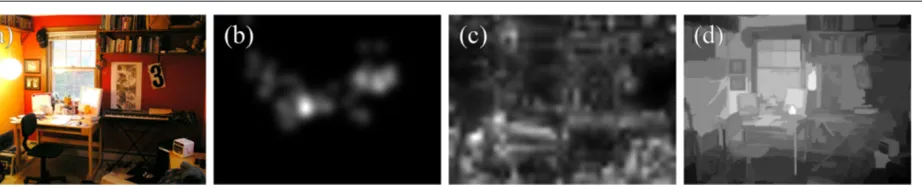
The bottom-up saliency detection methods can be broadly classified into local and global schemes. The local contrast-based methods measure the visual rarity with respect to the local neighborhoods using multi-scale image features [1,19,20]. The saliency maps generated by such methods usually highlight the object boundary. Fur-thermore, without knowing the scale of the salient object, the local methods may not detect the salient object accu-rately. On the contrary, the global contrast-based methods measure the saliency of a pixel by integrating its contrast to all pixels in the image [12,21,22]. Generally, the global methods can generate saliency maps with full resolution and evenly highlighted salient regions. These methods can achieve good accuracy of saliency detection in a scene which consists of a single salient object and a simple back-ground. However, it is hard to detect salient objects from complex scenes due to the global consideration. As shown in Figure 1, the pen container is the most salient accord-ing to the fixation density map from the MIT-1003 dataset [23], which shows the region attracting the attention of most subjects. The saliency map in Figure 1c highlights the object boundary, which is obtained from the local method [1]. The global method [22] cannot detect the container because the color of the container is similar to that of the wall and its contrast to all the pixels of the image is low, as shown in Figure 1d.

Figure 1Saliency detection in a complex scene.(a)Original image.(b)Human fixation density map.(c)Saliency map of the local method [1].(d) Saliency map of the global method [22].

In this paper, we focus on a bottom-up model of saliency detection, which is widely believed to be closely connected to the ubiquity of attention mechanisms in the early stages of biological vision [24]. In neuroscience, numerous stud-ies show that the neuronal response is elevated by the stimulus within the classical receptive field (the center), while stimuli presented in the annular window surround-ing the receptive field (the surround) inhibit the response [25]. According to the ‘center-surround’ mechanisms and the spatial frequency response of the human visual sys-tem (HVS) [26], we propose a saliency model based on the following principles of human visual attention:

1. Appearance distinctness between an object and its surroundings. It is generally considered that the response of neurons comes from the contrast of the center region and the surrounding regions [27]. For a pixelp which is inside an object, the pixel is salient if the object is distinct from its surroundings.

2. Unevenness of appearance within an object while appearance similarity within its surrounding region. For a pixelp inside a region (the center), the pixel is salient if the variability of the region is not too low since some intermediate spatial frequency stimuli may evoke a peak response [26]. Meanwhile, the stimuli from the surrounding region should be as weak as possible because the surround is antagonistic to the center and a stronger response will be evoked without the surrounding stimuli [25]. So, the surrounding region should have low variability. 3. Large object size. According to the

neuropsychological experiments, attentive response increases when the stimulus size is large and the object is attended [28]. If multiple objects have the same distinctness with respect to their surroundings, humans may pay attention to the larger object first.

These principles reflect the common human character-istics about saliency perception. For example, according to the visual experiments, the spatial frequency response of the HVS, which is similar to the response of a band-pass filter, has a peak response at about 2 to 5 cycles per

degree (cpd) and falls off at about 30 cpd [26]. As shown in Figure 2a, a cluttered image is hard to attract peo-ple’s attention. Principle 2 demands HVS to be sensitive to stimuli from the center and not at the surroundings in order to create stronger center-surround contrast and make the object attentive. In the experiments, we find that each of the principles contributes to the performance of the saliency detector.

Extending our previous work [29], we propose a novel method to measure visual saliency based on biologically plausible saliency mechanisms with a reasonable mathe-matical formulation. We define the saliency of an image region in a statistical way by means of the scatter matrix. For a pixel in an image, the center region and the sur-rounding region are defined as the regions centered at the pixel. For a center and a surrounding region, the saliency value is determined by two scatter matrices of the visual features. The first is the ‘within-classes scat-ter matrix’ SW which expresses the similarity between the features of the center region and the surrounding region. The second is the ‘between-classes scatter matrix’ SBwhich describes how the feature statistics in the cen-ter region diverge from those in the surrounding region. For a pixel, there exist many concentric regions with different radii, which have different prominence with respect to their surroundings. In order to detect the most salient objects in the scenes, the saliency support region of a pixel is explored, which is the most salient cen-ter region among all the concentric cencen-ter regions. In order to make the large object more salient, the saliency value is weighted using the radius of the saliency support region.

Figure 2Two types of images.(a)A cluttered image.(b)A concise image. The two people in image(b)attract our attention.

The proposed method is evaluated on three eye track-ing datasets which comprise natural images in different scenes and the corresponding human fixation data. Com-pared to 12 state-of-the-art methods and the human fixa-tion data, the experimental results show that our method outperforms all other methods in terms of receiver oper-ator characteristic (ROC) area metrics for the human fixation prediction task.

This paper is organized as follows: The related work is in Section 2. Section 3 describes the proposed method for saliency detection. The experimental results are provided in Section 4 to verify the effectiveness of the method. Finally, the conclusion is drawn in Section 5.

2 Related work

In the past few decades, a lot of bottom-up saliency-driven methods have been proposed in cognitive fields, which can be broadly classified as biologically inspired, purely computational, or an integration of the two [21].

Many attention models are based on the biologically inspired architecture proposed by Koch and Ullman [30], which is motivated from Treisman and Gelade’s feature integration theory (FIT) [31]. This structure explains the human visual search strategies, i.e., the visual input is firstly divided into several feature types (e.g., intensity, color, or orientation) which are explored concurrently, and then the conspicuities of the features are combined into a saliency or master map which is a scalar, two-dimensional map providing higher intensities for the most prominent areas.

According to this biologically plausible architecture, a popular bottom-up attention model is proposed by Itti et al. [1]. In Itti’s model, three multi-resolution extracted local feature contrasts, i.e., luminance, chrominance, and orientation, are mixed to produce a saliency map. Walther and Koch [19] extended Itti’s model to infer proto-object regions from individual contrast maps at different spatial scales. These models obtained good results in applications from computer vision to robotics [19,32].

In the last decade, many purely computational methods came up to model saliency with less biological motivation. Ma and Zhang [33] proposed a fuzzy growing method to extract salient objects based on local contrast analysis. Achanta et al. [21] estimated the center-surround con-trast by using a frequency-tuned technology. In order to solve the object scale problem, Achanta et al. extended their work by using a symmetric-surround method to vary the bandwidth of the center-surround filtering near image borders [34]. Hu et al. [35] presented a composite saliency indicator and a dynamic weighting strategy to estimate saliency. Hou and Zhang [36] extracted the saliency map from the spectral residual of the log-spectrum of an image. According to the global rarity principle of saliency, Zhai and Shah [37] and Cheng et al. [22] used the histogram-based method to detect the global contrast of a pixel or region. By filtering color values and position values, Perazzi et al. [38] computed the uniqueness and distri-bution to detect salient regions. Recently, based on a graph-based manifold ranking method, Yang et al. [39] detected saliency of the image elements by ranking the similarity to background and foreground queries. Li et al. [40] performed saliency detection by integrating the dense and sparse reconstruction errors of image regions. These state-of-the-art methods can extract salient regions effec-tively.

to simulate the information transmission among the neurons.

Besides Bruce’s work, some other saliency detectors also established models based on information theory. Itti and Baldi [42] presented a Bayesian definition of surprise to describe saliency. Gao and Vasconcelos [43] proposed a discriminant saliency detection model by maximizing the mutual information of the center and surrounding regions in an image. Klein and Frintrop [44] used the integral his-tograms to estimate the distributions of the center and surrounding region and expressed the saliency by the Kullback-Leibler divergence (KLD) of these distributions. Statistical theory has also gotten into the field of saliency detection. Zhang et al. [45] computed saliency based on the self-information of local image features using natural image statistics. Also using natural image statistics, Vigo et al. [46] detected salient edge based on ICA.

We implement the computation of saliency based on the statistics of local image regions. Our work is most closely related to the within-classes scatter matrix and between-classes scatter matrix in Fisher’s linear discriminant anal-ysis (LDA) which is commonly used for dimensionality reduction before later classification [47]. We use these two scatter matrices to measure the variability within/between the center and surrounding regions which are defined in Section 3.1. Furthermore, we compute the visual saliency based on principles 1 and 2.

Some methods detect saliency at a single spatial scale [33,35], while others combine feature maps at multiple scales to the final saliency map [1,19,20]. Without know-ing the scale of the object, these methods may not detect the most salient object accurately. The proposed method finds the saliency support region for a local area and computes the saliency of this region with respect to its surroundings to detect multiple salient objects adaptively.

3 Proposed method

In this section, we propose a computational method for saliency detection in images, which is performed in the CIELAB color space. We first define the center region and surrounding region that are used for the center-surround contrast computation. Secondly, a central stim-uli sensitivity-based model is proposed to compute the saliency of the center region. Then, the saliency support region of a given pixel is searched to mimic the maximum response of the receptive field in the neurophysiological experiment. Finally, we introduce the visual saliency map generation.

3.1 Center region and surrounding region

The saliency computation of the method is based on the selection of two regions, i.e., the center region and sur-rounding region. According to the center-surround mech-anism, the saliency of a pixel is determined by the contrast

between the center object (which the pixel belongs to) and the surrounding region. Withouta prioriinformation of the center object, we assume that it is approximately within a circular region centered at the pixel, which is referred to as the center region. In this paper, the sur-rounding region of the center region is defined as the con-centric annular region outside the center region, which has the maximal radius toward the nearest image border. For a pixel in the image, there are many center regions. As shown in Figure 3, three center regions for the center pixel of the circles are shown, which are the regions within the blue, purple, or red circles. The corresponding surround-ing regions are the annular regions between these circles and the outmost yellow circle.

3.2 Central stimuli sensitivity-based saliency model According to principles 1 and 2, the appearance distinct-ness between the object and its surrounding and the appearance similarity of each of them are key for visual saliency detection. In order to make an object prominent, the stimuli from the center region should make the HVS sensitive while the stimuli from the surrounding region should not. Following the band-pass characteristic of the spatial frequency response of the HVS [26], we measure the sensitivity in a statistics-theoretic way.

Inspired by the scatter matrices used in Fisher-LDA [47], we use the within-classes scatter matrix to measure the similarity of the center region, Rc, and the surrounding

region,Rs, which is defined as

SW=

n∈{1,2}

p∈Rn

xp−μn xp−μn T

(1)

whereR1denotes the regionRc,R2denotes the regionRs,

xpis the feature vector of pixelp(the vector contains the

intensity and color features in the experiments), andμn

is the mean feature vector of the region Rn_{. The matrix}

of each region is normalized by the number of the pix-els in the region. The eigenvalues of the scatter matrix are related to the spatial frequency of the region. If a region is flat, the pixels in the region concentrate on their mean. In other words, the pixels in the region are not scattered. For two flat regions, the eigenvalues ofSWare small. Accord-ing to principle 2, we define the sum of the eigenvalues of SWto be inversely proportional to the saliency value in the method. However, a flat center region with low frequency may get a large saliency value, which violates principle 2. In order to measure the sensitivity to the center stimuli, which has a peak response at an intermediate frequency [26], we modify (1) by weighting the matrix ofRc, which

can be represented as

SW=ωc

p∈R1

xp−μ1 xp−μ1 T

+

p∈R2

xp−μ2 xp−μ2 T

Figure 3Examples of center regions and surrounding region.Three center regions for the pixel in the circle center are shown, which are the regions within the blue, purple, or red circles. The corresponding surrounding regions are the annular regions between these circles and the outmost yellow circle.

whereωcis a empirically set parameter to control the

con-tribution of the similarity ofRcto the computed saliency

value. By settingω_cto 1, a flat center region may produce a large saliency value. Ifω_cis decreased, an uneven cen-ter region with a higher spatial frequency may generate a large saliency value. We will demonstrate in Section 4.5 that the weightω_cplays a significant role in the saliency computing.

To measure the difference ofRc andRs, the

between-classes scatter matrix is used, which is defined as

SB=

n∈{1,2}

(μn−μ) (μn−μ)T (3)

whereμ is the overall mean feature vector of the pixels inRc

Rs. For two regions which are distinct from each

other, the eigenvalues ofSBare large.

The saliency of a particular center region depends on the traces ofSWandSB, i.e., the sums of eigenvalues of the two scatter matrices, which is computed by

Sal(Rc)=

trace(SB) trace(SW)

. (4)

A center region which is distinct from its flat surrounding region has a high saliency value.

3.3 Saliency support region

As shown in Figure 3, many center regions exist for a pixel. Some of them are salient, such as the region within the blue circle, while some others are not, such as the regions within the red and purple circles. As mentioned in Section 2, some of the previous work preset multiple spatial scales or use a single scale to detect saliency, which may fail to find the salient object.

According to the spatial summation curves in the neuro-physiological experiments, when the visual stimuli cover the area of receptive field center, the neural responses reach the peak [48]. We believe that for a salient object, there exists a support to form the saliency quality, which

generates a peak response in the neuron. We attempt to find the support region which generates the most intensive saliency with respect to its surrounding region, referred to as the saliency support region.

We define the saliency support region of a pixel as the center region which has the largest saliency value using (4). The saliency support region, SSR, can be formulated as

SSR=arg max

Rc∈A

Sal(Rc) (5)

whereAis the set of all the possible center regions of a pixel. As shown in Figure 4, the saliency support region of the pixel in the middle of the flower is the region within the red circle, which consists of the stamens and has the largest saliency value with respect to its surround-ing region of flower petals and green leaves. Other center regions are less salient than the saliency support region. We use the saliency value of the saliency support region to represent the saliency of the center pixel of the SSR. The exploration of the saliency support region intends to measure the maximal saliency of pixels and find salient objects with different sizes. For a pixel, there are many possible center regions that need to be compared. In order to reduce computational expense, we reduce the candidate center regions by sampling their radii at a fixed interval in the implementation, i.e., only the regions with the sampled radii are compared.

3.4 Visual saliency map

Figure 4An example of the saliency support region.The region within the red circle is the saliency support region of the pixel in the middle of flower stamen, which has the largest saliency value with respect to its surrounding region of flower petals and green leaves.

by the radius of the saliency support region, which can be represented as

Sal(p)=Sal(SSR)·r(SSR) (6)

wherepis the center pixel of the saliency support region (SSR), andr(SSR) denotes the radius of SSR.

Instead of measuring the saliency values of all the pixels, we sample the pixels at an interval (e.g., 10 pixels) for com-putation reduction. The lattice of the sampled pixels is interpolated bilinearly and Gaussian filtered withσ =25

to generate the final saliency map of the image, as shown in Figure 6.

4 Experiments

In this section, we apply the proposed method on three public eye tracking datasets (two color image datasets and one gray image dataset) to evaluate the performance of human fixation prediction. These datasets comprise natural images, containing different objects and scenes, and the corresponding human fixations. The proposed

Figure 6An example of the saliency map.(a)Original image.(b)Lattice of the sampled pixels.(c)Saliency map generated by interpolation and filtering.

method is compared with the state-of-the-art bottom-up methods based on a well-known validation approach. The qualitative and quantitative assessments of detection results are reported.

4.1 Parameter setting

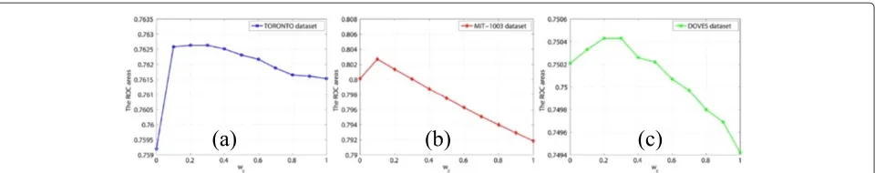
There is a parameter in the proposed method: the weight ω_cof the within-classes scatter matrix of the center region in (2). We set the weightω_c = 0.1 because it can obtain large areas under the ROC curves in the experiments on the three datasets. The relationship between the param-eter and the performance of the method is discussed in Section 4.5.

4.2 Experiments on BRUCE color image dataset

In the first experiment, we perform saliency computa-tions on the popular color image dataset introduced by Bruce and Tsotsos [11], which consists of 120 images in indoor and outdoor scenes, such as human objects, fur-niture, phones, fruits, cars, buildings, streets, etc. All the image sizes are 681×511 pixels. In the dataset, 20 sub-jects’ fixations are recorded for each image. To compare the saliency maps with the human fixations objectively, we use the popular validation approach as in [11]. The area under the ROC curve is used to quantitatively evaluate the performance of visual saliency detection.

We compare the proposed method with 12 state-of-the-art bottom-up saliency detection methods, i.e., Itti’s model (IT) [1], attention information maximization (AIM) [11], spectral residual (SR) [36], graph-based visual saliency (GB) [13], site entropy rate (SER) [41], context aware (CA) [49], salient region detection (AC) [20], max-imum symmetric surround (MSS) [34], region-based contrast (RC) [22], saliency filters (SF) [38], graph-based manifold ranking (MR) [39], and dense and sparse recon-struction (DSR) [40] which are listed in Table 1. These methods involve a variety of saliency models, such as biologically motivated (e.g., IT), computational (e.g., AC and MSS), frequency-based (e.g., SR), mixed (e.g., AIM and GB), local contrast (e.g., IT and AC), global contrast (e.g., RC), and state-of-the-art (e.g., SF, MR, and DSR) models. Some of the methods are used to predict human

fixations, such as AIM, GB, and SER, and some others show excellent performance in the salient region/object extraction task, such as RC, SF, MR, and DSR. For all these methods, we use the source codes or executable codes by the authors. The proposed method is implemented in Matlab.

Figure 7 qualitatively shows the comparison results of saliency maps for some test images of the BRUCE dataset. The original images are shown in Figure 7a, while the maps obtained from the state-of-the-art methods are given in Figure 7b,c,d,e,f,g,h,i,j,k,l,m, respectively. The results of the proposed method are shown in Figure 7n. The fixation density maps are shown in the final column, which are generated from the sum of 2D Gaussians cor-responding to each fixation point of all the subjects [11]. It can be seen that most of the methods can detect the single salient object in a simple scene, such as the sec-ond row. However, it is challenging for the images which

Table 1 The state-of-the-art methods

Algorithm name Reference Implementation code

Itti’s model (IT) Itti [1] Matlab code by Harel [13]

Attention information max. (AIM)

Bruce [11] Matlab code by author

Spectral residual (SR) Hou [36] Matlab code by author

Graph-based visual saliency (GB)

Harel [13] Matlab code by author

Site entropy rate (SER) Wang [41] Executable code by author

Context aware (CA) Goferman [49] Matlab code by author

Salient region detection (AC)

Achanta [20] Executable code by author

Maximum symmetric surround (MSS)

Achanta [34] Executable code by author

Region-based contrast (RC)

Cheng [22] Executable code by author

Saliency filters (SF) Perazzi [38] C code by author

Graph-based manifold ranking (MR)

Yang [39] Matlab code by author

Dense and sparse reconstruction (DSR)

Figure 7Examples of saliency maps over the BRUCE dataset.(a)Original images.(b to n)Saliency maps achieved by the methods IT [1], AIM [11], SR [36], GB [13], SER [41], CA [49], AC [20], MSS [34], RC [22], SF [38], MR [39], DSR [40], and the proposed method.(o)Human fixation density maps.

consist of multiple objects or complex scenes. The com-parison results show that our maps which are based on the biological perception mechanisms are more consis-tent with the human fixation density maps. For example, in the third image, the scene is a bit complex. There are some objects, e.g., the tomatoes, cup, and knife, on a mot-ley table mat. The two tomatoes have the stronger local contrast than the other objects. As a result, it is shown from the fixation density map that the tomatoes attract the attention of most of the subjects. However, most of the methods fail to do well. In the methods IT, AIM, SR, GB, and CA, saliency detection is performed by searching the high-frequency regions. So, the boundaries of the objects are detected as the most salient. In some methods, such as SER, MSS, and SF, the pixels in the cup, knife, or table mat are very salient due to the global consideration. The proposed method searches the saliency support region to explore the most salient region. So, the tomatoes are assigned the highest saliency value and recognized as the most salient region. Meanwhile, if multiple salient objects have the comparable local contrast, our method also can detect these objects. For example, for the eighth image, the two salient objects are detected by the proposed method.

In order to evaluate the quality of the proposed method, we perform a quantitative comparison by computing the salient degree between the extracted saliency map and the human fixations. The popular validation approach, the ROC area [11], is used to evaluate the performance of visual saliency detection. The results of ROC areas of

the compared methods on this dataset are shown in the second column of Table 2. Among the existing methods, the very recent method MR has the best fixation pre-diction performance on this dataset, whose ROC area is 0.7378. It shows that MR does well not only in the salient region detection task but also in this fixation pre-diction evaluation. However, it can be seen that the ROC

Table 2 The ROC areas on three eye tracking datasets

BRUCE MIT-1003 DOVES

Method dataset dataset dataset

IT [1] 0.5709 0.6835 0.5548

AIM [11] 0.6275 0.7662 0.6201

SR [36] 0.5315 0.6977 0.5429

GB [13] 0.5237 0.6857 0.5061

SER [41] 0.6632 0.7835 0.6716

CA [49] 0.6307 0.7585 0.6271

AC [20] 0.5520 0.6251 0.5312

MSS [34] 0.6107 0.6774 0.5530

RC [22] 0.6461 0.7568 0.6176

SF [38] 0.6601 0.7019 0.6492

MR [39] 0.7378 0.7766 0.7375

DSR [40] 0.7144 0.7908 0.7021

PMa _{0.7626 0.8027 0.7503}

a quantization threshold, i.e., the threshold classifies the locations in a fixation density map into fixations and non-fixations. So, different quantization thresholds lead to different results. To perform a fair comparison, we use the fixation points provided by the dataset as the ground truth for all the compared methods, i.e., only the points are fixa-tions and the rest are non-fixafixa-tions. The ROC areas of the compared methods are generated using the Matlab code provided by Harel et al. [13].

4.3 Experiments on MIT-1003 color image dataset We perform saliency computations on another color image dataset introduced by Judd et al. [23]. The MIT-1003 dataset contains 1,003 natural images of varying dimensions (the maximal dimension of the width and height is 1,024 pixels), along with human fixation data from 15 subjects. The images in this dataset contain differ-ent scenes and objects, as well as many semantic objects, such as faces, people, body parts, and text, which are not modeled by bottom-up saliency [23].

We compare the proposed method with the same 12 methods listed in Table 1 on this dataset. Comparison results of saliency maps for some of the test images are shown in Figure 8. The original images are shown in Figure 8a, while the results from the state-of-the-art methods are given in Figure 8b,c,d,e,f,g,h,i,j,k,l,m, respec-tively. The results of the proposed method are shown in Figure 8n, and the fixation density maps provided in the dataset are given in Figure 8o. For the fifth and seventh images that contain complex background, the global contrast-based methods, e.g., RC and SF, are apt to highlight the noise regions, e.g., shadows, and over-look the key regions. Some local contrast-based methods, such as IT, AIM, SR, GB, and CA, detect the bound-ary of objects as the most salient like their performance on the BRUCE dataset. Although some methods pre-set multiple scales, such as IT and AC, they cannot effectively detect salient objects in the complex scenes. Method SER performs better than other existing meth-ods. However, for the images with multiple objects, such as the sixth and seventh images, SER only detects one object. By following the biological perception mecha-nisms and exploring the saliency support region, the pro-posed method can achieve good performance to predict most of the fixations in the images that contain com-plex scenes and semantic objects. For example, in the fifth image, the proposed method detects the face of the

The results of ROC areas of the compared methods on this dataset are shown in the third column of Table 2. Among the existing methods, the very recent method DSR shows the best performance on this dataset. The proposed method achieves a slightly higher ROC area than DSR and also outperforms the state-of-the-art meth-ods on this human fixation dataset. We notice that the improvement of our method on this dataset is not as overt as on the BRUCE dataset. The main reason is that the MIT-1003 dataset contains many semantic objects which put forward challenges to the bottom-up models. The detected results by our method are based on the bottom-up contrast, which may diverge from the fixations of the subjects. Using some high-level features may improve the results.

4.4 Experiments on DOVES gray image dataset

In the third experiment, we test the proposed method on a gray image dataset, DOVES, which is introduced by van der Linde et al. [50]. The DOVES dataset contains 101 nat-ural images and the eye tracking data from 29 subjects. All the image sizes are 1, 024×768 pixels. Because the first fixations of each eye movement trace of the subjects are forced at the center of the image [50], these fixations are removed in the experiments.

Figure 8Examples of saliency maps over the MIT-1003 dataset.(a)Original images.(b to n)Saliency maps achieved by the methods IT [1], AIM [11], SR [36], GB [13], SER [41], CA [49], AC [20], MSS [34], RC [22], SF [38], MR [39], DSR [40], and the proposed method.(o)Human fixation density maps.

Figure 10The relationship between the ROC area and the weightωc.Results on(a)the BRUCE dataset,(b)the MIT-1003 dataset, and(c)the DOVES dataset.

human fixations well. It shows that the proposed method has a good ability to predict fixations even for gray images.

The results of ROC area of all the compared methods on the DOVES dataset are presented in the fourth col-umn of Table 2. Method MR shows the highest ROC area (0.7375) on this dataset compared to the previous meth-ods. The main reason is that most of the subjects tend to focus their fixations on the image center if there are no very prominent regions. Compared with MR, the pro-posed method achieves about 2% improvement of ROC area. It shows that the proposed method outperforms the state-of-the-art methods on fixation prediction for gray images.

4.5 Discussion

In our model, the parameter ωc is designed to

deter-mine the region of which frequency will be assigned a high saliency value. If ω_c is set to 1 and 0, the regions with very low and high frequency will be assigned high saliency values, respectively. According to the HVS princi-ples, the very low and high frequency regions may weaken the response of the HVS. So, an inappropriate value ofω_c will lead to the wrong detection, i.e., the ROC area may be small.

Figure 10 shows the relationship between the ROC area and the weight ωc in (2) on the three datasets.

Gener-ally, when the weightωcis bigger than 0.3, the ROC area

decreases as the weight increases. That is to say, the salient objects are not necessarily flat according to the evalua-tion based on the human fixaevalua-tion data. On the contrary, if no constraints are imposed on the similarity of the center region, i.e.,ωc=0, the ROC area drops, especially on the

BRUCE dataset, the ROC area in Figure 10a is the lowest whenω_c= 0. That is to say, if the center region is rather cluttered, it may not attract human attention. This result is consistent with the spatial frequency response of the HVS [26]. The curves in Figure 10 are similar to the mirror of the spatial frequency response curve, which show that the response reaches a maximum when the spatial frequency

gets an intermediate frequency, ω_c is between 0.1 and 0.3, while it falls off rapidly at higher frequency, namely ωc = 0. The response decreases slowly as the frequency

decreases to DC, i.e.,ωc = 1, from the intermediate

fre-quency. It is worth noting that our model is biologically plausible. It is difficult to denote the spatial frequency by specific values ofωc.

The performance improvement of the proposed method in the fixation prediction experiments verifies the effec-tiveness of the scatter matrix-based saliency computation and the saliency support region exploration. However, since we use the pixel-wise processing manner and the SSR is searched for every processed pixel, the method is computationally expensive. We therefore adopt the sub-sampling method to reduce the cost. The average running time on the BRUCE dataset to generate the saliency map is 60.63 s when measured on an Intel 3.20-GHz CPU with 3-GB RAM in Matlab implementation. In the future, we will study the superpixel-based processing to make the algorithm more efficient.

5 Conclusions

Competing interests

The authors declare that they have no competing interests.

Acknowledgements

This work was partially supported by NSFC (No. 61201274), National High Technology Research and Development Program of China (863 Program, No. 2012AA011503), and Fundamental Research Funds for the Central Universities (No. ZYGX2012J025).

Received: 27 July 2013 Accepted: 17 June 2014 Published: 24 June 2014

References

1. L Itti, C Koch, E Niebur, A model of saliency-based visual attention for rapid scene analysis. IEEE Trans. Pattern Anal. Mach. Intell.20(11), 1254–1259 (1998)

2. S Kastner, LG Ungerleider, Mechanisms of visual attention in the human cortex. Ann. Rev. Neurosci.23, 315–341 (2000)

3. HE Egeth, S Yantis, Visual attention: control, representation, and time course. Ann. Rev. Psychol.48, 269–297 (1997)

4. R Desimone, J Duncan, Neural mechanisms of selective visual attention. Ann. Rev. Neurosci.18, 193–222 (1995)

5. H Li, KN Ngan, Saliency model based face segmentation in

head-and-shoulder video sequences. J. Vis. Commun. Image Represen. 19(5), 320–333 (2008)

6. H Li, KN Ngan, Learning to extract focused objects from low DOF images. IEEE Trans. Circuits Syst. Video Technol.21(11), 1571–1580 (2011) 7. KC Liu, Prediction error preprocessing for perceptual color image

compression. EURASIP J. Image Video Process.2012, 3 (2012) 8. D Mahapatra, Y Sun, Rigid registration of renal perfusion images using a

neurobiology-based visual saliency model. EURASIP J. Image Video Process.2010, 195640 (2010)

9. J You, G Liu, A novel attention model and its application in video analysis. Appl. Math. Comput.185(2), 963–975 (2007)

10. M Mancas, B Gosselin, B Macq, Perceptual image representation. EURASIP J. Image Video Process.2007, 098181 (2007)

11. N Bruce, JK Tsotsos, Saliency based on information maximization. Adv. Neural Inform. Process. Syst.18, 155–162 (2006)

12. W Luo, H Li, G Liu, KN Ngan, Global salient information maximization for saliency detection. Signal Process.: Image Commun.27(3), 238–248 (2012) 13. J Harel, C Koch, P Perona, Graph-based visual saliency. Adv. Neural Inform.

Process. Syst.19, 545–552 (2006)

14. H Li, KN Ngan, A co-saliency model of image pairs. IEEE Trans. Image Process.20(12), 3365–3375 (2011)

15. F Meng, H Li, G Liu, KN Ngan, Object co-segmentation based on shortest path algorithm and saliency model. IEEE Trans. Multimedia14(5), 1429–1441 (2012)

16. H Li, F Meng, KN Ngan, Co-salient object detection from multiple images. IEEE Trans. Multimedia15(8), 1896–1909 (2013)

17. T Liu, J Sun, NN Zheng, X Tang, HY Shum, Learning to detect a salient object, inProceedings of IEEE Conference on Computer Vision and Pattern Recognition (CVPR)(Minneapolis, 18–23 June 2007), pp. 1–8

18. J Li, Y Tian, T Huang, W Gao, Multi-task rank learning for visual saliency estimation. IEEE Trans. Circuits Syst. Video Technol.21(5), 623–636 (2011) 19. D Walther, C Koch, Modeling attention to salient proto-objects. Neural

Netw.19(9), 1395–1407 (2006)

20. R Achanta, F Estrada, P Wils, S Süsstrunk, Salient region detection and segmentation, inProceedings of International Conference on Computer Vision Systems (ICVS), vol. 5008 (Santorini, 12–15 May 2008), pp. 66–75 21. R Achanta, S Hemami, F Estrada, S Süsstrunk, Frequency-tuned salient

region detection, inProceedings of IEEE Conference on Computer Vision and Pattern Recognition (CVPR)(Miami, 20–25 June 2009), pp. 1597–1604 22. MM Cheng, GX Zhang, NJ Mitra, X Huang, SM Hu, Global contrast based

salient region detection, inProceedings of IEEE Conference on Computer Vision and Pattern Recognition (CVPR)(Colorado Springs, 20–25 June 2011), pp. 409–416

23. T Judd, K Ehinger, F Durand, A Torralba, Learning to predict where humans look, inProceedings of IEEE International Conference on Computer Vision (ICCV)(Kyoto, 27 Sept–4 Oct 2009), pp. 2106–2113

24. D Gao, N Vasconcelos, Decision-theoretic saliency: computational principles, biological plausibility, and implications for neurophysiology and psychophysics. Neural Comput.21, 239–271 (2009)

25. KA Sundberg, JF Mitchell, JH Reynolds, Spatial attention modulates center-surround interactions in macaque visual area V4. Neuron61(6), 952–963 (2009)

26. DH Kelly, Motion and vision.I. Stabilized images of stationary gratings. J. Opt. Soc. Am.69, 1266–1274 (1979)

27. JR Cavanaugh, W Bair, JA Movshon, Nature and interaction of signals from the receptive field center and surround in macaque V1 neurons. J. Neurophysiol.88(5), 2530–2546 (2002)

28. K Herrmann, L Montaser-Kouhsari, M Carrasco, DJ Heeger, When size matters: attention affects performance by contrast or response gain. Nat. Neurosci.13(12), 1554–1559 (2010)

29. L Xu, H Li, L Zeng, Z Wang, G Liu, Saliency detection using a central stimuli sensitivity based model, inProceedings of IEEE International Symposium on Circuits and Systems (ISCAS)(Beijing, 19–23 May 2013), pp. 945–949 30. C Koch, S Ullman, Shifts in selective visual attention: towards the

underlying neural circuitry. Hum. Neurobiol.4, 219–227 (1985) 31. AM Treisman, G Gelade, A feature-integration theory of attention. Cogn.

Psychol.12, 97–136 (1980)

32. S Frintrop, E Rome, HI Christensen, Computational visual attention systems and their cognitive foundation: a survey. ACM Trans. Appl. Percept.7, 6:1–6:39 (2010)

33. YF Ma, HJ Zhang, Contrast-based image attention analysis by using fuzzy growing, inProceedings of ACM International Conference of Multimedia (Berkeley, 2–8 Nov 2003), pp. 374–381

34. R Achanta, S Süsstrunk, Saliency detection using maximum symmetric surround, inProceedings of IEEE International Conference on Image Processing (ICIP)(Hong Kong, 26–29 Sept 2010), pp. 2653–2656 35. Y Hu, X Xie, W Ma, L Chia, D Rajan, Salient region detection using

weighted feature maps based on the human visual attention model, in Proceedings of Fifth Pacific Rim Conference on Multimedia(Tokyo, 30 Nov–3 Dec 2004), pp. 993–1000

36. X Hou, L Zhang, Saliency detection: a spectral residual approach, in Proceedings of IEEE Conference on Computer Vision and Pattern Recognition (CVPR)(Minneapolis, 18–23 June 2007), pp. 1–8

37. Y Zhai, M Shah, Visual attention detection in video sequences using spatiotemporal cues, inProceedings of ACM International Conference of Multimedia(Santa Barbara, 23–27 Oct 2006), pp. 815–824

38. F Perazzi, P Krähenbühl, Y Pritch, A Hornung, Saliency filters: contrast based filtering for salient region detection, inProceedings of IEEE Conference on Computer Vision and Pattern Recognition (CVPR)(Providence, 16–21 June 2012), pp. 733–740

39. C Yang, L Zhang, H Lu, X Ruan, MH Yang, Saliency detection via graph-based manifold ranking, inProceedings of IEEE Conference on Computer Vision and Pattern Recognition (CVPR)(Portland, 23–28 June 2013), pp. 3166–3173

40. X Li, H Lu, L Zhang, X Ruan, MH Yang, Saliency detection via dense and sparse reconstruction, inProceedings of IEEE International Conference on Computer Vision (ICCV)(Sydney, 1–8 Dec 2013), pp. 2976–2983 41. W Wang, Y Wang, Q Huang, W Gao, Measuring visual saliency by site

entropy rate, inProceedings of IEEE Conference on Computer Vision and Pattern Recognition (CVPR)(San Francisco, 13–18 June 2010), pp. 2368–2375

42. L Itti, P Baldi, Bayesian surprise attracts human attention. Adv. Neural Inform. Process. Syst.19, 547–554 (2006)

43. D Gao, N Vasconcelos, Bottom-up saliency is a discriminant process, in Proceedings of IEEE International Conference on Computer Vision (ICCV)(Rio de Janeiro, 14–20 Oct 2007), pp. 1–6

44. DA Klein, S Frintrop, Center-surround divergence of feature statistics for salient object detection, inProceedings of IEEE International Conference on Computer Vision (ICCV)(Barcelona, 6–13 Nov 2011), pp. 2214–2219

45. L Zhang, MH Tong, TK Marks, H Shan, GW Cottrell, SUN: a Bayesian framework for saliency using natural statistics. J. Vis.8(7), 1–20 (2008)

visual eye movements. Spat. Vis.22(2), 161–177 (2009)

doi:10.1186/1687-5281-2014-31

Cite this article as:Xuet al.:Saliency detection in complex scenes.EURASIP Journal on Image and Video Processing20142014:31.

Submit your manuscript to a

journal and benefi t from:

7Convenient online submission 7Rigorous peer review

7Immediate publication on acceptance 7Open access: articles freely available online 7High visibility within the fi eld

7Retaining the copyright to your article