DOI10.1186/2190-8567-4-2
R E S E A R C H Open Access
A Density Model for a Population of Theta Neurons
Grégory Dumont·Jacques Henry·Carmen Oana Tarniceriu
Received: 15 January 2013 / Accepted: 3 September 2013 / Published online: 17 April 2014
© 2014 G. Dumont et al.; licensee Springer. This is an Open Access article distributed under the terms of the Creative Commons Attribution License (http://creativecommons.org/licenses/by/2.0), which permits unrestricted use, distribution, and reproduction in any medium, provided the original work is properly cited.
Abstract Population density models that are used to describe the evolution of neural populations in a phase space are closely related to the single neuron model that de-scribes the individual trajectories of the neurons of the population and which give in particular the phase-space where the computations are made. Based on a transforma-tion of the quadratic integrate and fire single neuron model, the so-called theta-neuron model is obtained and we shall introduce in this paper a corresponding population density model for it. Existence and uniqueness of a solution will be proved and some numerical simulations are presented. The results of existence are compared to previ-ous results of existence or nonexistence (burst) for populations of leaky integrate and fire neurons.
1 Introduction
It is a big challenge to find the most appropriate mathematical model to describe the electrical activity of populations of neurons; it should, in the first place, give
G. Dumont (
)·J. HenryInstitut de Mathématiques de Bordeaux, Université Bordeaux 1, 351 cours de la Libération, 33405 Talence cedex, France
e-mail:[email protected] Present address:
G. Dumont
Physics Department, University of Ottawa, 150 Louis Pasteur, Ottawa, Ontario, Canada K1N 6N5 J. Henry
INRIA Bordeaux Sud Ouest, 200 avenue de la vieille tour, 33405 Talence cedex, France e-mail:[email protected]
C.O. Tarniceriu
a realistic view of the very complex brain activity and be able to describe the emergent phenomena that are observed in vivo, but in the same time, it should keep a certain simplicity that would help to analytically solve it and to numerically implement it.
Our attention has been kept by the so-called population density approach that has been successfully used to describe the evolution of physiologically structured pop-ulation in many areas of biology, and in particular, in neuroscience. A poppop-ulation density model will track down the evolution of a density function of the population in the state space, which is determined by the structuring variable. In theoretical neu-roscience, the concept of a probability density function has been already extensively used ([1–3]). A step forward, though, was made by applying this concept to model interactions of large populations of sparsely connected neurons ([4–7]). The connec-tion between probability-density approach and populaconnec-tion density approach is based on the observation that, for a large population of similar neurons, the probability density can be interpreted as a population density ([4,6]). For a method to derive population density models, we refer to [6], where an illustrative exemplification is given for the case of integrate-and-fire neurons. Here, the effect of the synaptic con-nections has been modeled as a jump in the state variable, the membrane potential in this case, when a neuron of the population receives a synaptic input. For more sim-ulations of networks of integrate-and-fire neurons via population density models, we also refer to [8] and [9]. Another method can be found in [10] where a population density equation has been derived for a population of SRM (spike-response model) neurons with escape noise. A well-posedness result for a population density model of Leaky Integrate-and-Fire (LIF) neurons can be found in [11]. The approach proved to be an useful tool in analyzing special behaviors of neural populations, such as the existence of equilibrium solution ([12]), or the emergence of synchronization of neurons ([13–15]).
It is somehow usual to apply the population density formalism to populations of integrate-and-fire neurons, due to the simplicity of the model and to the possibility to express the firing rate in terms of the population density function. We have chosen in this paper to consider a large homogeneous population of neurons that are char-acterized by the theta-neuron model ([16]). As it is known, the theta neuron model, or Ermentrout–Kopell model, is an alternative version of the Quadratic Integrate-and-Fire (QIF), which is the simplest spiking neuron model. In contrast to the leaky integrate-and-fire model, the QIF model does have a spike generation mechanism, which makes it suitable for us to describe the internal state of a population density function of neurons. Nevertheless, the use of the equivalent theta-neuron model is preferable since it is a continuous version of the QIF model, and the state variable varies in a finite domain. We will come back in the first section of this paper with more details about this subject.
We therefore use the population density formalism in this paper to derive a pop-ulation density model for a poppop-ulation of theta-neurons and we shall prove the well-posedness of the model by a method similar to those used in [11] or [14] in the case of populations of leaky integrate-and-fire neurons. The main difference between these cases and the one considered in this paper is due to the different expressions of the firing rates of the populations.
a homogeneous population of neurons characterized by the quadratic and-fire model. Based on the Ermentrout–Kopell transformation, the quadratic integrate-and-fire can be written in its equivalent form in terms of a new variable called the phase of a neuron. We next introduce a population density model for the population of neurons that is structured by their phase instead of their membrane’s potential. We continue by proving the well-posedness of the model; in the non-connected case, i.e., when all the neurons of the population receive only an external stimulus, the result we prove is global. In the case of a connected population, we prove a global well-posedness result under an assumption that has sense from a biological point of view. If the above specified assumption is not taken into consideration, the result is only local.
We end this paper by presenting some numerical simulations for the population density model that we introduced, which are compared to direct Monte Carlo simu-lations.
2 Quadratic Integrate-and-Fire Neurons: Population Density Approach
The quadratic integrate-and-fire model was introduced in [17] and consists in an or-dinary differential equation that models the evolution in time of the membrane’s po-tential, and a reset mechanism. We consider in this paper a model that describes the dynamics of a (QIF) neuron that receives external stimuli:
d
dtv(t )=v 2(t )+I
b+h+∞j=1δ(t−tj)
Ifv= +∞ thenv= −∞. (1)
Here,v(t )represents the potential of the neural membrane at time t,tj are the ar-rival times of external impulses, and the effect of the reception of a spike at neuron’s synapse has been modeled as a jump of sizeh of the potentialv. The jump is pos-itive (respectively negative) if the spike is received from an excitatory (respectively inhibitory) source. Due to the quadratic term,vcan reach infinity in finite time. The time whenvreaches the infinity value is considered as the time when the neuron is emitting a spike and the potential of the membrane is instantaneously reset to−∞. The parameterIbplays a key role in the dynamics of the (QIF) model of neuron’s potential (see [18,19], and [20] for details).
Let us now introduce the population density function such that
v2
v1
p(t, v)dv=Fraction of neurons having at timet
the potential of the membranev∈ [v1, v2]
.
Thenp(t, v)is the relative density of the population that has at timet the potential of the membranevand one has
+∞
We shall follow below the same assumptions and derivation formalism as those used in [4,6,7] for the case of leaky integrate-and-fire neurons, assumptions that will be shortly reminded below.
One of the main hypotheses used to obtain a population density model is that the population is homogeneous, i.e., all the neurons of the population have the same properties, and, in our case, are individually described by the model (1).
The spikes received by the neurons of the population, either from internal or exter-nal sources, are supposed to be uniformly distributed in the population, and letσ (t )
be the average spike arrival rate. Given a statev, the flux flowing through the statev
is supposed to be composed of two parts: a drift flux due to the continuous evolution determined by the (QIF) model (1) and a flux due to synaptic connections among the neurons of the population. The flux due to synaptic connections is generated by all the neurons thatjumpfrom the statev−hinto the statev whenever an electric impulse is received. Thus, the total flux is defined as
J(t, v)=v2+Ib
p(t, v)+σ (t )
v
v−hp(t, w)dw. (2)
Therefore, the evolution in time of the density functionpis given by
∂
∂tp(t, v)= − ∂
∂vJ(t, v) (3)
which can be written equivalently as
∂
∂tp(t, v)+
Quadratic integrate-and-fire
∂ ∂v
v2+Ib
p(t, v)+σ (t )
Excitation
p(t, v)−p(t, v−h)=0. (4)
A periodic boundary condition for the flux is imposed next, which is consistent with the reset mechanism of the single neuron model (1):
lim v→−∞
v2+Ib
p(t, v)= lim v→+∞
v2+Ib
p(t, v). (5)
Due to the boundary condition, one can check easily the conservation property of Eq. (4) by simple integration on the interval(−∞,+∞),
d dt
+∞
−∞ p(t, v)dv=0. (6)
Letr(t )be the firing rate of the population, that is, the flux throughv= +∞and
Jthe average connection per neuron
r(t )= lim v→+∞
v2+Ib
p(t, v). (7)
Fig. 1 Scheme of a population under an external influence without conduction delay. The population receives a known external influenceσ0(t ), and
produces the activityr(t ). The feedback is instantaneous and given byJ r(t )
Fig. 2 Scheme of a population
under an external influence with conduction delay. The population receives a known external influenceσ0(t )from an
excitatory population of neurons, and produces an activityr(t )—the firing rate of the population. The feedback is then given by
J0tα(u)r(t−u)du
the neurons in the same population. The second term can be considered in two ways: either we neglect the synaptic conduction delays within the population (Fig.1), in which caseσis written as
σ (t )=σ0(t )+J r(t ), or we take into account synaptic delays (Fig.2) and write
σ (t )=σ0(t )+J
t
0
α(u)r(t−u)du, (8)
with
∞
0
α(u)du=1, (9)
whereαis a delay density function.
We can now give the model in its complete form:
⎧ ⎪ ⎪ ⎪ ⎪ ⎪ ⎪ ⎪ ⎪ ⎪ ⎪ ⎪ ⎪ ⎨ ⎪ ⎪ ⎪ ⎪ ⎪ ⎪ ⎪ ⎪ ⎪ ⎪ ⎪ ⎪ ⎩
∂
∂tp(t, v)+ ∂ ∂v((v
2+I
b)p(t, v))
=σ (t )(p(t, v−h)−p(t, v)), (t, v)∈(0,+∞)×(−∞,+∞) σ (t )=σ0(t )+J
t
0α(s)r(t−s)ds, t≥0
r(t )=limv→+∞(v2+Ib)p(t, v), t≥0 limv→−∞(v2+Ib)p(t, v)
=limv→+∞(v2+Ib)p(t, v), t≥0
p(0, v)=p0(v), v∈(−∞,+∞).
In the model above, the case of instantaneous reception of the impulses can be ob-tained by takingα=δ(0).
Note that if the initial condition satisfies−∞+∞p0(v)dv=1, then the solution to the nonlinear problem (10) also satisfies−∞+∞p(t, w)dw=1.
In our paper,σ0 stands for the rate of the Poisson spike train that each neuron receives from an external source, which is not explicitly modeled. The rateσ0 is then considered as given. The case of a probability density model where the Pois-son spike train is approximated by the sum of a deterministic baseline and a white noise has been considered in [21]. In the paper [22], the authors derived an explicit formula of the firing rate of a noisy quadratic integrate-and-fire neuron with and with-out the synaptic dynamics. It is possible to look at this formula as the second-order approximation of the firing rate of a neural network where each neuron receives an independent Poisson spike train.
In the paper [23], the authors study the firing rate of the noisy quadratic integrate-and-fire neuron receiving an oscillatory input. To this end, the authors used the so-called linear response theory. The theory is not really adapted to a neural network where each neuron receives an independent Poisson spike train since the transfer function cannot be computed explicitly.
3 A Population Density Model for Theta Neurons
We shall shortly recall the derivation of the theta-neuron model (Ermentrout–Kopell). Let us consider a non-connected (QIF) neuron, i.e., its membrane potential is given by
d
dtv(t )=v 2(t )+I
b
Ifv= +∞ thenv= −∞. (11)
Then, by taking the transformation
θ=2 arctanv+π, (12)
one can prove directly by changing the variablev=tanθ−π2 in the first equation of (11), that the evolution in time of the new variableθ, calledthe phase, is given by
d
dtθ (t )=(1+cosθ )+(1−cosθ )Ib. (13)
Obviously, the following correspondences take place:
v−→ +∞ ⇔ θ−→2π,
v−→ −∞ ⇔ θ−→0.
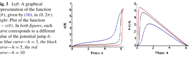
Fig. 3 Left: A graphical representation of the function s(θ ), given by (16), in(0,2π ).
Right: Plot of the function θ−s(θ ). Inboth figures, each curve corresponds to a different value of the potential jumph:
the blue curve—h=3,the black curve—h=5,the red
curve—h=10
Now, if we consider next a coupled neuron which is described by the model (1), corresponding to the jump in potential generated by an impulse arrival
v−→v+h, (14)
we have a phase shift (see [24]), given by
θ−→2 arctan
h+tan
θ−π
2
+π.
Or, equivalently, if a neuron receiving an impulse has a jump in potential
v−h−→v, (15)
then, the phaseθchanges correspondingly as
s(θ ):=2 arctan
tan
θ−π
2
−h
+π−→θ. (16)
By continuity, we extend the formula atθ=0 by
0−→0,
which means that a neuron which receives an impulse at the time of spike emission will not have a phase shift. The evolution of the functionswith respect to phaseθis exemplified in Fig.3.
Then the evolution of the phase of a connected neuron is given by
d
dtθ (t )=(1+cosθ )+(1−cosθ )Ib
+
2 arctan
h+tan
θ−π
2
+π−θ
+∞
j=1
δ(t−tj). (17)
Based on the transformation of the model (1) into the model (17), we intend to obtain a corresponding population density model for a population of neurons charac-terized by their phaseθ. The advantages of doing so are obvious: first of all, through this transformation, the state spacev∈(−∞,+∞)is transformed into a finite one
the statev will be replaced by a continuous flow through the state 2π, which will influence the expression of the firing rate of the population, as it can be seen below.
As before, if we denote byq(t, θ )the density of neurons having phaseθat timet, then
θ2
θ1
q(t, θ )dθ=Fraction of neurons with phaseθ∈ [θ1, θ2]at timet
,
and one can assume once again that
2π 0
q(t, θ )dθ=1.
As in the previous section, we assume the homogeneity of the population and the uniform distribution of the average reception rate over the neurons of the population. Similarly, we consider the flux flowing now through a stateθas formed of the drifting flux due to the continuous evolution of the phase of the neurons due to (13), and the flux determined by the phase shifting generated by the arrival of synaptic impulses:
J(t, θ )=f (θ )q(t, θ )+σ (t )
θ
s(θ )
q(t, y)dy, (18)
where
f (θ )=(1+cosθ )+(1−cosθ )Ib,
s(θ )=2 arctan
tan
θ−π
2
−h
+π. (19)
Then, corresponding to Eq. (4), we obtain
∂
∂tq(t, θ )+
Theta neuron
∂ ∂θ
f (θ )q(t, θ )=σ (t )
Excitation
s(θ )qt, s(θ )−q(t, θ ), (20)
where the functionsf andsare defined by (19).
Due to the fact that the second term of the flux (18) does not affect the neurons at the firing state, the boundary condition becomes in this case:
f (0)q(t,0)=f (2π )q(t,2π ) ⇔ q(t,0)=q(t,2π ).
The same argument is applied to obtain the expression of the firing rate, which was defined as the flux through the phase 2π:
r(t )=f (2π )q(t,2π )
=2q(t,2π ). (21)
flux, we have here the opposite case, since only the drift flux influences the rate of neurons at the firing phase. Another major difference is that, in our model, the firing rate does not explicitly depend on the average reception rateσ as it is the case in the leaky integrate-and-fire population density models ([6,11]).
Using the boundary condition, and integrating (20) on the domain(0,2π ), one can easily check the conservation property of Eq. (20).
Therefore, the evolution in time of the density functionq(t, θ )is described by the following system:
⎧ ⎪ ⎪ ⎪ ⎪ ⎪ ⎪ ⎪ ⎪ ⎪ ⎨ ⎪ ⎪ ⎪ ⎪ ⎪ ⎪ ⎪ ⎪ ⎪ ⎩
∂
∂tq(t, θ )+ ∂
∂θ(f (θ )q(t, θ ))
=σ (t )(s(θ )q(t, s(θ ))−q(t, θ )), t >0, θ∈(0,2π ) σ (t )=σ0(t )+J
t
0α(s)r(t−s)ds, t≥0
r(t )=2q(t,2π ), t≥0
q(t,0)=q(t,2π ), t≥0
q(0, θ )=q0(θ ), θ∈ [0,2π],
(22)
where, as before, if we takeαas a given function of time, we obtain the case where synaptic delays are considered, whereas forα(t )=δ(t ), we obtain the case of instan-taneous synaptic transmission.
The models (10) and (22) are obviously related through the following relation between the density functionspandq:
p(t, v)dv=q(t, θ )dθ ∀t∈(0,+∞).
4 Existence and Uniqueness of the Solution
In this section, we shall prove the existence and uniqueness of the solution to problem (22). This will be done first in the linear case, i.e., whenσ (t )=σ0(t )(withσ0a given function), and later in the general nonlinear case.
4.1 The Linear Case
In this subsection, we are going to prove the global existence of a unique solution for the linear version of the model. Assuming thatJ is zero, which corresponds to the case when the neurons of the population are not connected but each of them receives an external inputσ0, the model reduces to the following problem:
⎧ ⎪ ⎪ ⎪ ⎪ ⎨ ⎪ ⎪ ⎪ ⎪ ⎩
∂
∂tq(t, θ )+ ∂
∂θ(f (θ )q(t, θ ))
=σ (t )(s(θ )q(t, s(θ ))−q(t, θ )), t >0, θ∈(0,2π ) q(t,0)=q(t,2π ), t >0
q(0, θ )=q0(θ ), θ∈ [0,2π],
(23)
Theorem 1 Letσ ∈C(0,+∞)a bounded function and the initial condition q0∈
C[0,2π] a periodic function.Then there exists a unique positive solution to prob-lem(23),q∈C([0,+∞)× [0,2π]),which is periodic with respect to the second argument.Furthermore,the firing rater(t )is bounded by an exponential:for some
λ >0,
r(t )≤Ceλt.
LetXλ, whereλ >0 will be specified later, be defined by
Xλ=
p∈C[0,+∞)× [0,2π]/p(t,0)=p(t,2π ),
ande−λtp(t,·)L∞[0,2π]<∞.
We endowXλwith the following norm:
p = ess sup t∈[0,+∞(
e−λ(t )p(t,·)L∞[0,2π]. (24)
Let us introduce onXλthe mappingF defined by
F:Xλ→Xλ
m→q, (25)
whereq is the solution to the problem
⎧ ⎪ ⎪ ⎪ ⎪ ⎨ ⎪ ⎪ ⎪ ⎪ ⎩
∂
∂tq(t, θ )+ ∂
∂θ(f (θ )q(t, θ ))
=σ0(t )(s(θ )m(t, s(θ ))−q(t, θ )), t >0, θ∈(0,2π )
q(t,0)=q(t,2π ), t≥0
q(0, θ )=q0(θ ), θ∈ [0,2π].
(26)
In order to prove Theorem1, we shall use the Banach’s fixed-point theorem for the applicationF. First of all, let us introduce more rigorously the notion of a solution to our system. First, we define acharacteristic lineas the solution to
˙
θ (t )=fθ (t ), θ (0)=θ0, (27) where
f (θ )=(1+cosθ )+(1−cosθ )Ib.
Sincef is a Lipschitz continuous function on[0,2π], there exists a unique solution to problem (27) that gives the characteristic curve that starts from a pointθ0att=0, and it can be extended to every t >0 by periodicity, due to the periodicity off. Actually, it will be more helpful to define the characteristic in the equivalent way, as follows: for everyt≥0 fixed, for everyθ∈ [0,2π], there exists a single curve, let us denote itc[(0, θ0)](t ), such that
˙
c(0, θ0)
(t )=fc(0, θ0)
(t ), c(0, θ0)
(t )=θ, c(0, θ0)
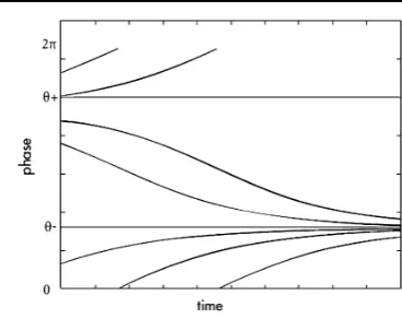
Fig. 4 The evolution in time of the characteristic lines in the caseIb<0
We have used here a different notation for a curve starting from a point(0, θ0)in order to avoid confusions. Due to the properties of the functionf, we will have that, for any given point(t, θ )there is a unique initial point(0, θ0).
The computations below were considered for all the casesIb<0, Ib=0 and
Ib>0. The way the characteristics behave in time in each case is different, but this does not affect the results stated below. We just remind that forIb<0, Eq. (27) has two equilibria: a stable attractor and a nonstable equilibrium. In Fig.4, we represented the evolution in time of the characteristics in the caseIb<0. ForIb=0, the equation has one equilibrium, which is a saddle node, while for the caseIb>0, (27) has no equilibrium.
The main problem for defining a solution on these lines is to be sure that they do not cross in order not to lose the diffeomorphic property. By a simple computation one can find that
∂c[θ0](t )
∂θ0 = exp
t
0
fc[θ0](τ )
dτ
, (29)
therefore we have that for any finitet, ∂c[θ0](t )
∂θ0 is strictly positive, and then the
char-acteristics starting from different points do not cross. Nevertheless, depending on the sign offthe above derivative can go asymptotically to 0.
On the characteristic lines, we can rewrite (26) as an ordinary differential equation
d dtq
t, c(0, θ0)
(t )=σ0(t )s
c(0, θ0)
(t )mt, sc(0, θ0)
(t )
−σ0(t )+f
c(0, θ0)
(t )qt, c(0, θ0)
(t ).
Since the domain[0, T]×[0,2π]is covered by the above defined characteristic lines, we have that for every(t, θ )∈ [0, T] × [0,2π],
q(t, θ )=qt, c(0, θ0)
(t )
=e−
t
0(σ0(s)+f(c[(0,θ0)](s)))dsq
0(0, θ0)
+ t
0
e−
t
u(σ0(s)+f(c[(0,θ0)](s)))ds
×σ0(u)s
c(0, θ0)
(u)mu, sc(0, θ0)
By direct computation one gets that
fc(0, θ0)
(t )=(Ib−1)sin
c(0, θ0)
(t ), f(θ )≤ |Ib−1|, (31)
and
s(θ )= 2
[tan((θ−π )/2)−h]2+1·
1
cos2((θ−π )/2)· 1 2
= 1
[sin((θ−π )/2)−hcos((θ−π )/2)]2+cos2((θ−π )/2)≤β. (32) Let us denote in the following
σ0=inf
t≥0σ0(t ), σ0=supt≥0σ0(t ). (33) Thus, one has
exp − t 0
σ0(s)+f
c(0, θ0)
(s)ds ≤ expt−σ0+ |1−Ib|
:=exp{t M}, ∀t≥0.
Let us prove the contraction property of the mapF and takem1,m2two solutions to the problem; then
F (m1)
t, c(0, θ0)
(t )−F (m2)
t, c(0, θ0)
(t )
≤ t
0
exp(t−u)Mσ0(u)s
c(0, θ0)
(u)
×m1
u, sc(0, θ0)
(u)−m2
u, sc(0, θ0)
(u)du
≤βσ0
t
0
exp(t−u)M
×m1
u, sc(0, θ0)
(u)−m2
u, sc(0, θ0)
(u)du.
Thus, multiplying the last inequality bye−λt and taking the ess sup with respect tot, one gets that
F (m1)−F (m2)≤
βσ0
λ+Mm1−m2
1−expt (−λ+M)
≤ βσ0
λ+σ0− |1−Ib|
(m1−m2),
which implies that, forλ > βσ0−σ0+ |Ib−1|,
F (m1)−F (m2)≤K(m1−m2), K <1,
4.2 The Nonlinear Case
Let us go back now to the general model (22). Below, we prove the existence and uniqueness of a solution locally in time. Then, under an assumption regarding the number of connections per neuron and the delay kernel, the global in time existence is proved.
Theorem 2 Letσ0andαbe two functions ofC(0,+∞)and the initial conditionq0
be a periodic function ofC[0,2π].Then one can findT >0 such that there exists a unique positive solution to the nonlinear problem(22), q∈C([0, T] × [0,2π]),
which is periodic with respect to the second argument.
In the following, the computations will be made in the space
X=C
[0, T] × [0,2π], · ∞,
whereC stands for the functions that are continuous in time and continuous and periodic in phase. Let us define onXthe mapGby
G:X→X
m→q,
whereq is the solution to the problem
⎧ ⎪ ⎪ ⎪ ⎨ ⎪ ⎪ ⎪ ⎩
∂
∂tq(t, θ )+ ∂
∂θ(f (θ )q(t, θ ))=σ (t )[s(θ )m(t, s(θ ))−m(t, θ )]
σ (t )=σ0(t )+Jf (2π )
t
0α(t−s)m(s,2π )ds
q(t,0)=q(t,2π ) q(0, θ )=q0(θ ).
The proof will use the standard Banach–Picard fixed-point theorem applied to the mapG with respect to the usual norm onL∞([0, T] × [0,2π]). Below · will denote the norm inL∞.
Let(t, θ )∈ [0, T] × [0,2π]. As before, we define a characteristicc[(0, θ0)](t )as a solution to (28) and write the problem along these curves as
d dtq
t, c(0, θ0)
(t )
= −fc(0, θ0)
(t )qt, c(0, θ0)
(t )
+σ (t )sc(0, θ0)
(t )mt, sc(0, θ0)
(t )−mt, c(0, θ0)
(t ). (34)
For any fixed bounded functionsmandσ, one can find a unique solutionq by inte-grating (34)
q(t, θ )= qt, c(0, θ0)
(t )
= e−
t
0f(c[(0,θ0)](s))dsq
+ t
0
e−
t
uf(c[(0,θ0)](s))ds
×σ (u)sc(0, θ0)
(t )mu, sc(0, θ0)
(t )−mu, c(0, θ0)
(t )du
:=G(m). (35)
It remains therefore to show that the application
m→G(m),
withGdefined by (35), andσ given by
σ (t )=σ0(t )+2J
t
0
α(t−s)m(s,2π )ds, (36)
has a fixed point.
To prove the invariance of a ball inX, let us takeR a positive real number to be fixed later on, andm∈Xsuch thatm ≤R. Then, for everyT >0:
σ ≤ σ0 +2J TαR. (37)
Choosing for nowT ≤2J1αR, the last relation yields:
σ ≤ σ0 +1. First note that, definingMT as
MT = ess sup 0≤u≤t≤T
exp
−
t
u
fc[θ0](s)
ds
,
we get that
MT <exp
T|1−Ib|
. (38)
Next, taking the absolute value in (35), we obtain by using the relations (32) and (38):
G(m)≤expT|1−Ib|
q0 +T
σ0 +1
[βR+R]
≤expT|1−Ib|
q0 +
1 2Jα
σ0 +1
(β+1),
where we have also used the fact thatT ≤2J1αR.
Let us assume that the time interval is chosen less than a given valueT0, and take
T ≤min
T0, 1 2JαR
,
forRdefined as a
R=expT0|1−Ib|
q0 +
1 2Jα
σ0 +1
Then
T ≤min
T0,
1
exp(T0|1−Ib|){2Jαq0 +(σ0 +1)(β+1)}
,
which shows that the invariance of the ball property takes place locally in time. Let us go now to the contraction property and take solutions m1, m2∈X two solutions to (35). We denote byσ1 andσ2the corresponding quantities defined by (36) tom1andm2. Then
G(m1)−G(m2)
t, c(0, θ0)
(t )
≤expT0|1−Ib|
× t
0
σ1(τ )s
c(0, θ0)
(τ )
×m1
τ, sc(0, θ0)
(τ )−m2
τ, sc[θ0](τ )
+sc(0, θ0)
(τ )m2
τ, sc(0, θ0)
(τ )σ1(τ )−σ2(τ )dτ
+ t
0
σ1(τ )m1
τ, c(0, θ0)
(τ )−m2
τ, c(0, θ0)
(τ )
+m2
τ, c(0, θ0)
(τ )σ1(τ )−σ2(τ )dτ
.
Using the fact that the solutions are elements ofX, the bound forσ given by (37), and, again, the relations (32) and (38), we obtain:
G(m1)−G(m2)≤exp
T0|1−Ib|
T(β+1)σ0 +1
m1−m2
+(β+1)2RJ Tαm1−m2
≤TexpT0|1−Ib|
(β+1)σ0 +2
m1−m2, where we have also used 2J T Rα<1. Choosing nowT such that
T <min
T0,
1
exp(T0|1−Ib|)(β+1)(σ0 +2)
,
1
exp(T0|1−Ib|){2Jαq0 +(σ0 +1)(β+1)}
,
one gets the conclusion on the interval[0, T].
Theorem 3 Let us assume the same hypothesis as in Theorem2.We assume further-more that2Jα<1.Then there exists an unique solution to problem(22)that is global in time.
corresponding lengths of the intervals will be denoted by{li}ni=1. We will also use, for convenience, the following notations:γ= |1−Ib|,k1=2Jαandk2=(σ0+ 1)(β+1). Using these notations, we have obtained that there exists a unique solution onB(0, R1)with
R1:=exp(γ l1)
q0 +
k2
k1
on the interval[0, T1], whereT1is chosen such that
l1<min
T0,
1
exp(γ l1)(β+1)(σ0 +2)
, 1
exp(γ l1){k1q0 +k2}
. (39)
Let us consider now the problem on the next interval,[T1, T2]with the initial condi-tionq01(θ )=q(T1, θ ). We shall concentrate our attention on the third term in (39) since it explicitly depends on the initial condition. Then considering again the same applicationG, given by (35), and following the same computations, we obtain that
G(m)≤expl2|1−Ib|
q01 +
1 2Jα
σ0 +1
(β+1).
Since
q01 ≤R1, we get that
G(m)≤expγ (l1+l2)
q0 +2
k2
k1
,
andT2is chosen such that
l2≤exp
γ (l1+l2)
k21q0 +k1k2+k2
.
By induction, it follows that, for thenth interval, the following relations should hold:
Rn=exp
γ
n
i=1
li
q0 +n
k2
k1
and
ln≤
1
exp{γni=1li}[k1nq0 +k2
n−1 i=0ki1]
. (40)
In order to get this, we shall choose the time intervals such that
ln=
c n,
withca positive constant to be specified later. By doing so, we obtain the result on the interval[0, Tn]of length
n
Using
n
i=1 1
i <1+logn,
it follows that
exp
γ
n
i=1
li
≤exp{cγ}ncγ.
Also, fork1<1
k1n<1,
n−1
i=0
k1i =1−k
n 1 1−k1
. (41)
Then we can bound
1
exp{γni=1li}[k1nq0 +k2
n−1 i=0k1i]
≥ 1
ecγncγ[q
0 +k2/(1−k1)]
,
and choosingcsuch thatcγ <1, it follows that for someN0 1
ecγncγ[q
0 +k2/(1−k1)]≥
c
n, forn≥N0,
which completes our proof.
We shall end with a remark regarding a special case of the nonlinear problem, for which the global result obtained in the linear case holds. Suppose that we consider the case of delayed average reception rate, i.e.,
σ (t )=σ0(t )+
t
0
α(t−s)q(s,2π )ds
and we assume that the delay functionαis zero in a neighborhood of the origin[0, τ]. When integrating along the characteristics on the interval[0, τ], the solution of our problem is given by the solution of the linear problem considered in the first subsec-tion. Next, reiterating the procedure on the intervals[kτ, (k+1)τ],k=1,2, . . ., and having in mind that
(k+1)τ kτ
α(k+1)τ−sq(s,2π )ds=
τ
0
α(s)q(k+1)τ−s,2πds=0
andqis already calculated on the interval[0, (k−1)τ], one gets a global solution for this special case, which is given by the solution of the linear problem.
5 Numerical Results
method applied to the theta-neuron model. To solve numerically (22), we write the first equation of the system in a conservative form
∂
∂tq(t, θ )+ ∂
∂θJ(t, θ )=0,
with the fluxJ(t, v)given by
J(t, θ )=f (θ )q(t, θ )+σ (t )
θ
s(θ )
q(t,θ )d˜ θ˜
:=F (t, θ )+I (t, θ ),
whereI (t, θ )stands for the integral part of the flux andF (t, θ )for the drift part of the flux.
Denoting bytthe time step and byθthe phase step, we define
θk=kθ, tn=nt, qkn=q
tn, θk
,
Fkn+1/2=Ftn, θk+1/2
, Ikn+1/2=Itn, θk+1/2
, Jnk+1/2=Jtn, θk+1/2
.
For the discretization of (22), we use a first-order explicit in time scheme given by
qkn+1=qkn− t θ
Jnk+1/2−Jnk−1/2
=qkn− t θ
Fkn+1/2−Fkn−1/2− t θ
Ikn+1/2−Ikn−1/2.
The drift numerical fluxFk+n 1/2was reconstructed by using the upwind method (see [25] for details of the upwind numerical reconstruction) and the integral partIkn+1/2
was approximated by using a first order reconstruction.
The simulations of the model (22) presented in Fig.5show the evolution in time of the phase distribution of the neural population. The blue curve in the plots cor-responds to the Monte Carlo simulation and the black curve to the finite differences scheme discretization of (22). In the first plot, upper left of Fig.5, the initial repar-titionq0, which is a truncated Gaussian, is represented. Under the influence of the external impulsesσ0(t ), the jump process present in the model (22) takes place. The density seems to reach an equilibrium that is shown in the last plot of Fig.5. Unfor-tunately, we have not proved theoretically the existence of a steady state, which is subject to our future research. In Fig.6, we show the evolution in time of the firing rate of the populationr(t )under a constant external influence and in Fig.7the firing rate of the population under an oscillatory external influence. Again, it can be noticed that under a constant influence, the firing rate seems to converge toward a steady state.
6 Discussion and Conclusion
Fig. 5 Simulations of the model (22).The figuresgive the repartition of the population at different instants in time:t=0,t=0.1,t=0.5,t=0.6. For each instant,the two plots in the figuresrepresent the same densityq(t, θ )obtained by two different methods: the Monte Carlo method—blue curve, and the finite differences scheme approach for the model (22)—black curve. The initial Gaussian repartitionq0is
repre-sented in theupper left plot. The simulations have been obtained for a constant external influenceσ0=20,
the potential jump size—h=5, the coupling parameter—J=3 and the basic current—Ib= −1.The last
figureshows the repartition at the final timet=3, which evidences a convergence toward an equilibrium repartition
Fig. 6 Simulation of the evolution in time of the firing rater(t )for a constant external influenceσ0=20;
the potential jump size ish=5, the coupling parameter—J=3 and the basic current—Ib= −1. The
initial condition was taken as a Gaussian repartition
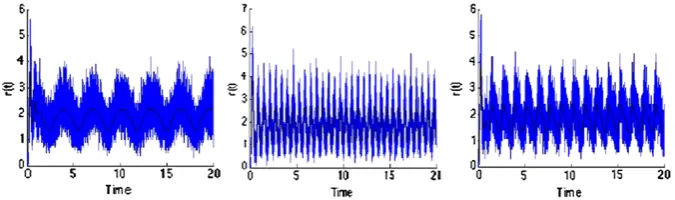
Fig. 7 Simulations of the model in the case when the initial condition is a Gaussian.The figures
rep-resent the evolution in time of the firing rater(t )of the model for a non constant external influence σ0(t )=I0+I1sin(ωt ). Inthe first plotI0=10,I1=10,ω=2, inthe second plotI0=10,I1=10,
ω=5 and inthe third plotI0=10,I1=10,ω=10. The potential jump size ish=5, the coupling
the behavior of populations of neurons. The population density approach leading to partial differential equations is suited for very large populations of neurons; we think that mathematical studies on the qualitative behavior of population density models may help for the choice of the particular single neuron model used to describe the internal state of the neurons of the population, and give insights on the results. In par-ticular, the possibility of burst of the firing rate corresponding to a synchronization of the neurons, as opposed to a regular activity, is of interest to neuroscientists.
We have highlighted a qualitative difference between the population density ap-proach applied to a population of theta-neurons, and the same apap-proach applied to populations of LIF neurons. In [11], it was proved that a global solution exists for the LIF population density approach equation with no delay and the firing rate remains bounded in the case whereJ <1. On the other hand, in [14] it was shown that forJ
andσ0large enough, for any initial condition there will be a burst in finite time: The firing rate goes to infinity.
In the present study of populations of theta-neurons, we consider only the case with conduction delay. The condition for existence of a global solution (no burst) involves the product of the number of connectionsJ and the maximum of the delay repartitionα. In order to satisfy this condition for largeJ, the delay kernelαshould spread over the time interval in order to decrease its maximum. So, it is possible to exhibit populations with the sameJ that will burst in finite time with the LIF model but will have a regular behavior on an infinite horizon with the QIF model with a different delay repartition.
As it is known, the formal threshold imposed in the LIF model is defined as the value at which an action potential is initiated, and the firing rate of the population density models in this case is defined as the flux passing through this threshold. In our case, the neurons of the population are supposed to transmit the electrical signal at the peak value, instead of the value at which the initiation of a spike occurs, which is actually theθ+root of the model (19). Therefore, the firing rate in our model de-pends only on the drifting flux through the phase 2π. This fact allowed us to obtain a global well-posedness result in the general case of the model. But the same fact does not allow to use the same argument as in [14] to study the conditions of bursting. Fur-thermore, in all the simulations that we have done, the synchronization phenomenon have not been observed in the case of a theta-neurons population.
Competing Interests
The authors declare that they have no competing interests.
Authors’ Contributions
In this paper, we have introduced a population density model for a population of theta-neurons. The global well-posedness of the model has been proved in the case when the neurons of the population are not con-nected but receive an external stimulation and, under a special assumption, in the case when connections among the neurons of the population are taken into account.
This seems to be the case in the simulations of the model and, as far as we know, the existence of a unique equilibrium solution to the model (22) is not proved.
Our main goal is to find an analytical description based on the model presented here for the occurrence of interesting behaviors, such as the synchronization of the neurons of the population. This will allow us to find the proper conditions that lead to such a behaviors and maybe, a way to control it.
All authors had an equal contribution to the theoretical part of the paper. The first author carried out the numerical simulations. All authors read and approved the final manuscript.
Acknowledgements The second and third authors were members of the project LEA Math-Mode Projet
Franco-Roumain. The first author has been financially supported by Conseil Régional d’Aquitaine.
References
1. Wilbur W, Rinzel J:A theoretical basis for large coefficient of variation and bimodality in
neu-ronal interspike interval distributions.J Theor Biol1983,105(2):345-368.
2. Kuramoto Y:Collective synchronization of pulse-coupled oscillators and excitable units.Physica D, Nonlinear Phenom1991,50:15-30.
3. Abbott LF, van Vreeswijk C:Asynchronous states in networks of pulse-coupled oscillators.Phys Rev E1993,48:1483-1490.
4. Knight B, Manin D, Sirovich L:Dynamical models of interacting neuron populations in visual
cortex.Robot Cybern1996,54:4-8.
5. Knight BW:Dynamics of encoding in neuron populations: some general mathematical features.
Neural Comput2000,12:473-518.
6. Omurtag A, Knight B, Sirovich L:On the simulation of large population or neurons.J Comput Neurosci2000,8:51-63.
7. Nykamp DQ, Tranchina D:A population density approach that facilitates large-scale modeling
of neural networks: analysis and an application to orientation tuning.J Comput Neurosci2000,
8:19-50.
8. Apfaltrer F, Ly C, Tranchina D:Population density methods for stochastic neurons with realistic
synaptic kinetics: firing rate dynamics and fast computational methods.Netw Comput Neural
Syst2006,17:373-418.
9. Cai D, Tao L, Rangan A, McLaughlin D:Kinetic theory for neuronal network dynamics.Commun Math Sci2006,4:97-127.
10. Gerstner W, Kistler W:Spiking Neuron Models. Cambridge: Cambridge University Press; 2002. 11. Dumont G, Henry J:Population density models of integrate-and-fire neurons with jumps:
well-posedness.J Math Biol2012.
12. Sirovich L, Omurtag A, Knight B:Dynamics of neuronal populations: the equilibrium solution.
J Appl Math2000,60:2009-2028.
13. Sirovich L, Omurtag A, Lubliner K:Dynamics of neural populations: stability synchrony.Netw Comput Neural Syst2006,17:3-29.
14. Dumont G, Henry J:Synchronization of an excitatory integrate-and-fire neural network.Bull Math Biol2013,75(4):629-648.
15. Garenne A, Henry J, Tarniceriu O:Analysis of synchronization in a neural population by a
popu-lation density approach.Math Model Nat Phenom2010,15:5-25.
16. Ermentrout GB, Kopell N:Parabolic bursting in an excitable system coupled with a slow oscilla-tion.SIAM J Appl Math1986,46:233-253.
17. Latham P, Richmond B, Nelson P, Nirenberg S:Intrinsic dynamics in neuronal networks. I. The-ory.J Neurophysiol2000,83:808-827.
18. Izhikevich EM:Dynamical Systems in Neuroscience. Cambridge: MIT Press; 2007.
19. Ermentrout B: Ermentrout–Kopell canonical model. Scholarpedia 2008. doi:10.4249/ scholarpedia.1398.
20. Eftimie R, de Vries G, Lewis MA:Weakly nonlinear analysis of a hyperbolic model for animal
group formation.J Math Biol2009,59:37-74.
21. Fourcaud N, Brunel N:Dynamics of the firing rate probability of noisy integrate and fire neurons.
22. Brunel N, Latham P:Firing rate of noisy quadratic integrate-and-fire neurons.Neural Comput
2003,15:2281-2306.
23. Fourcaud-Trocme N, Hansel D, van Vreeswijk C, Brunel N:How spike generation mechanisms
determine the neuronal response to fluctuating inputs.J Neurosci2003,23(37):11628-11640.
24. McKennoch S, Voegtlin T, Bushnell L:Spike-timing error backpropagation in theta neuron
net-works.Neural Comput2009,21:9-45.