R E S E A R C H
Open Access
Mice endplate segmentation from
micro-CT data through graph-based
trabecula recognition
Shi-Jian Liu
1†, Zheng Zou
2†, Jeng-Shyang Pan
1,3,4*and Sheng-Hui Liao
5Abstract
Though segmentation of spinal column from medical images have been intensively studied for decade, most of the works were concentrated on the segmentation of the vertebral body and arch, instead of the endplate. Recently, the increasing study on degeneration analysis of vertebra and intervertebral disc (IVD) make endplate segmentation as important as others. While the accurately segmentation of mice endplate from micro computed tomography (CT) images is challenging. The major difficulties include potential high system payload and poor run-time efficiency resulting from high-resolution micro-CT data, highly complicated and variable shape of the vertebra tissues, and the ambiguous segmentation boundary due to the similarity of spongy structures inside both the endplate and its adjacent vertebral body. To solve the problems, the core idea of the proposed method is to identify trabeculae between the endplate and the body through a graph-based strategy. In addition, in order to reduce the data
complexity, an endplate-targeted region of interest (ROI) extraction method is introduced according to the analysis of spatial relationship and variety of bone density of vertebra. Furthermore, shape priori of endplate in both
two-dimensional and three-dimensional are extracted to assist in the segmentation. Finally, an iterative cutting procedure is implemented to produce the final result. Experiments were carried out which validate the performances of the proposed method in terms of effectiveness and accuracy.
Keywords: Vertebral endplate, Trabecular bone, Segmentation, Harmonic field, Graph cuts, Micro-computed tomography
1 Introduction
Demanded by image-based spine assessment, biomechan-ical modeling and surgery simulation, segmentation of spinal column from medical images have been intensively studied for decades. In former researches, most of the works were concentrated on segmenting vertebral tis-sues such as the body and arch, while vertebral endplate segmentation were rarely mentioned. However, endplate is as important as the others. As a transitional zone between the intervertebral disc (IVD) and vertebra, it not only plays an important role in containing the adjacent
*Correspondence:[email protected]
†Shi-Jian Liu and Zheng Zou contributed equally to this work. 3College of Computer Science and Engineering, Shandong University of Science and Technology, 266590 Qindao, China
4Department of Information Management, Chaoyang University of Technology, Taizhong, Taiwan
Full list of author information is available at the end of the article
disc, distributing applied loads evenly to the underlying vertebra, but also serves as a semi-permeable interface that allows the transfer of water and solutes, preventing the loss of large proteoglycan molecules from the disc [1, 2]. Recently, it is also believed that there has a close relationship between the harm of endplate and osteoporo-sis [3]. Therefore, endplate segmentation could become an important pre-requisite of vertebra/IVD degeneration analysis and many other applications, which is a major motivation of this work.
Up to now, endplate segmentation from computed tomography (CT) images accurately is still a challenging task in practice, which relies heavily on knowledge, expe-rience, and manual works [4]. The main difficulties can be concluded as follows.
• Potential high system payload and poor run-time efficiency. The average thickness of endplate is
generally less than 80μm; therefore, a high-resolution imagery such as the micro-CT technique is required in order to achieve a high-accuracy segmentation. While, high resolution often leads to high system payload and poor run-time efficiency. • Highly complicated and variable shape of the
vertebra tissues. The shape of vertebra including the endplate, body and arch are highly complicated and variable. For example, the mice vertebra mice we test have transverse processes relatively longer and of larger curvature comparing to the human’s. Therefore, mice vertebral body and arch are more likely to be interrupted with each other; it is more difficult to separate them properly. Besides, existing algorithms designed for human vertebrae may not be suitable for our case anymore.
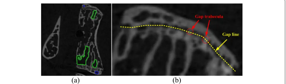
• Ambiguous segmentation boundary. Both the endplate and body are composed of spongy
cancellous bone (see blue and green region marked in Fig.1a), which makes the segmentation boundary ambiguous. Though there exists a gap area (labeled with a yellow dotted line in Fig.1b) between them, however, the gap is considerably narrow and divided by trabeculae, which means it is difficult to find a proper continuous curve as a segmentation boundary.
As we mentioned above, though few works could be found on endplate segmentation, plenty of researches have been done to achieve detection and segmentation of vertebrae [5–9], spinal canals [10], and spinal cord [11].
For the purpose of separating the neighboring vertebrae roughly, Zhao et al. [12] proposed a neighboring point rat-ing method based on constructrat-ing membership grade to form a virtual plane to cut adjacent processes. The method proposed by Kim et al. [9] searches a ray emitted from the stared point among the center axis of the spine and further
construct a three-dimensional (3D) surface by propagat-ing the ray to detect the accurate gap area between two processes.
A common strategy to reduce the data complexity is by limiting the algorithm applied to a relatively small region of interest (ROI) [13]. In order to identify the ROI, Athertya et al. [5] extract the Harris corners [14] among the possible vertebra region to detect the vertebra range. However, the detection needs several interactions and training in advance, meanwhile the accuracy of detec-tion depends on the selecdetec-tion of multi-stage seed points. Cheng et al. [6] detect the vertebra region by a proba-bilistic map computed from a voxel-wise classifier and use mean shift algorithm to estimate the ROI after annota-tions.
In our work, we also need to isolate individual vertebra from a given vertebral column, to extract the ROI for data complexity reduction, while more importantly, to segment the endplate, and we made it in a endplate-targeted way. Specifically, taking micro-CT images as input, we aim to develop an intelligent framework to accurately segment the endplate from the others. And the core idea is to recognize the trabeculae (e.g., marked by red circles in Fig.1b) within the narrow gap formed by the endplate and its adjacent vertebral body by a graph-based algorithm. The proposed framework can be separated into four parts, which are (1) pre-processing, (2) priori shape extraction, (3) gap trabecula detection, and (4) trabecula cutting and refining. Particularly, we firstly isolate each vertebra and identify the ROI for endplate in a top-down basis (Section2.1). Secondly, shape priori in both 2D and 3D are introduced to offer constraints for later graph cuts based trabeculae recognition (Section2.2). After that, a graph will be constructed based on mask skeletonization before the graph cuts based trabeculae recognition (Section2.3). Finally, we find an optimal cutting strategy to remove the
redundant connections properly (Section2.4). An accu-rate result can be achieved after these processes, which is ready for subsequent operations such as the 3D recon-struction.
2 Material and methods
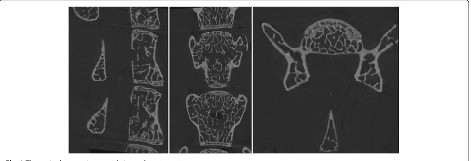
The experimental data we used were collected from the animal laboratory of spinal surgery of the Xiangya Hospital. Micro-CT technique is adopted due to the high-quality imagery requirement. To capture the data, mice of different ages were fixed in a slot scanned by a Bruker SkyScan1172 micro-CT scanner. The in-plane resolution of the image is 7.27μm×7.27μm, and the slice spacing is 7.27μm. Figure 2 demonstrates a typical data of the inputs, which contains 4 lumbar vertebrae.
2.1 Pre-processing
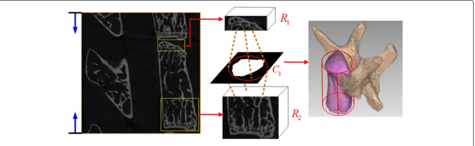
The aim of the pre-processing is to get proper ROI for the endplates. In this work, a top-down strategy which consists of three steps as shown in Fig.3is proposed to achieve the goal from coarse to fine.
The first step is to isolate the vertebra from each oth-ers. Other than finding separation lines or surfaces such as the method proposed by Kim et al. [9], thanks to the high resolution of micro-CT image and unconnected spa-tial relationship among different vertebrae, this step can easily be done by 3D region growing on the mask resulting from a Otsu threshold.
The second step finds out ROI for endplate within each axial slices. Due to the shape complexity mentioned above, it is normally impossible to completely cut off the ver-tebral arch by planes as proposed in existed methods [12, 15]. To remove useless regions as many as possible, an optimal cylinder will be computed automatically in our method to meet the quasi-cylindrical shape of the verte-bral body as shown in the right of Fig.4. The cylinder can be obtained by topology analysis of the vertebra beginning
from both the top and bottom part to the center part in axial planes slice by slice as indicated by blue arrows in Fig.4. Because in this way, we could find two regions indicated byR1 andR2 in Fig.4 which cover the entire
endplate. Then, based on the projection of bone regions withinR1 andR2, we can easily find a circle (e.g.,C1 in
Fig.4) which can be used to define the target cylinder. The last step produces the finest ROI by further con-firming the proper range of the axial slices. It travels each slice in the way as described in the second step, while other than analyzing the topology, bone densityρ(Ii) of each slice i will be calculated according to Eq. 1, and then the variation of bone density will be used to find the rightful indexes.
ρ(Ii)=
NF(Ii)
AF(Ii)×
100% (1)
whereAF(Ii)is the area (measured by number of pixels) of the entire vertebral region within sliceIi, whileNF(Ii) denotes the region where identified as the bone tissue withinAF(Ii)(e.g., the colored region of slice in Fig.5a).
The effect of this method lies in the fact that, as shown in Fig.5a, the top layer of endplate is much denser than the other parts. For example,ρ(Ia) > ρ(Ib) > ρ(Ic) > ρ(Id). With the computed data, a chart, as illustrated in Fig.5b, can be used to find the desirable range. The horizontal axis of the chart is the slice index, the vertical axis is the bone density accordingly. For the case shown in Fig.5b,
P1 and P2 will be chosen as the bounds of the range. Because, along with the direction of the horizontal axis,
ρ(IP1) reaches the first peak and the variation of bone
density aroundIP2become very small.
2.2 Shape priori extraction
It is well known that shape priori could be very useful because the constraints they represent could be important
Fig. 3The workflow of the proposed pre-processing
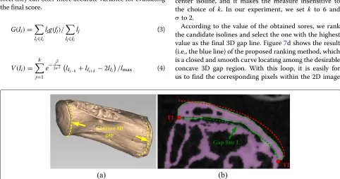
guidance for the segmentation. As for endplate segmenta-tion, there are two kinds of shape priori according to our observation. The first one is that there appears a concave gap between the endplate and the adjacent body, which can be observed from its 3D geometry. We use the yellow dotted line in Fig.6a to show this 3D shape priori. The sec-ond one is the shape similarity between the internal and external edge of endplate, which can be approximated by the green and red dotted line in Fig.6b respectively.
As we mentioned, the core idea of our method is to find and cut the trabeculae within the narrow gap within 2D image as shown in Fig. 6b; therefore, it is better for us to have some priori knowledge of the 2D gap, which described by a gap lineL(i.e., the green dotted line shown in Fig. 6b) in our method. To identify L, two terminal points (i.e.,T1 andT2) and the curve between them are
used.
Fortunately, with the first shape priori, an optimal 3D loop can be found by a harmonic field based method introduced in Section 2.2.1, which is useful for locating
T1andT2. While, with the second shape priori, a fitting
method is presented in Section2.2.2to approximate the shape ofL.
2.2.1 Terminal point identification
In our method, we solve the 2D terminal point identifica-tion problem from a 3D point of view, namely, a harmonic
field -based method as presented in our previous works [16,17] is adopted to find an optimal 3D loop laying on the vertebra mesh surface reconstructed from ROI intro-duced above. Figure7a demonstrates such a reconstructed mesh model.
Generally speaking, a harmonic field Ø is a scalar field attached to each mesh vertexes which satisfies Ø = 0, where is the Laplacian operator. Basic steps of the harmonic field based method include (1) designat-ing a proper weightdesignat-ing scheme, (2) calculatdesignat-ing Ø by a least square sense, and (3) choosing a desirable line from the isolines uniformly sampled from Ø. We adopt most part of the method from our former works, from which details such as the methodology and parameter setting can be found. Major differences between this method and the previous one lays in the following two aspects.
Firstly, when adopting least square method to solve the Poisson equationØ = 0, we use boundary constraints as illustrated in Fig. 7b, where the blue and red spheres indicate mesh vertexes of Dirichlet condition [18] equal to 1 and 0 respectively. Figure 7c shows all the isoline candidates.
Secondly, we proposed a ranking method to select the optimal isoline from the candidates through a score func-tionScore(Ii)of theith isolineIi defined by Eq.2, which takes two factors including the field gradient magnitude
Fig. 5Endplate region extraction.aAxial views (right) of four typical slices of index a, b, c, and d (left).bBone density variation among a sequence of slices. The horizontal axis is the slice index, the vertical axis is the bone density value accordingly,P1 andP2 indicate the range of the result
G(Ii)and the shape variance among the local regionV(Ii) into consideration.
Score(Ii)=G(Ii)×V(Ii) (2) where G(Ii) and V(Ii) meets Eqs. 3 and4 respectively. These two factors reflect both the variance along the indi-vidual isoline and among the local isoline region; there-fore, they can offer more accurate variance for evaluating the final score.
G(Ii)=
lj∈Ii
ljg(fj)/
lj∈Ii
lj (3)
V(Ii)= k
j=1
e−
j2
2σ2 l
Ii−k+lIi+k−2lIi
/lmax (4)
Letfjbe thejth triangle whereIipath through, thenljand
g(fj) denote the length and corresponding gradient ofIi withinfjrespectively. For the shape variance factorV(Ii), we take the isoline Ii as the center, and select the pre-vious and nextk isolines as the local region,Ii+k is the previouskth isoline,Ii−k is the next kth isoline.lmax is
the maximum length of the candidate isolines. The Gaus-sian convolution is used to design the different weight for neighboring isolines with different distances from the center isoline, and it makes the measure insensitive to the choice of k. In our experiment, we set k to 6 and
σto 2.
According to the value of the obtained sores, we rank the candidate isolines and select the one with the highest value as the final 3D gap line. Figure7d shows the result (i.e., the blue line) of the proposed ranking method, which is a closed and smooth curve locating among the desirable concave 3D gap region. With this loop, it is easily for us to find the corresponding pixels within the 2D image
Fig. 7Processes of the harmonic field based 3D shape priori extraction scheme.aThe 3D mesh model reconstructed from the ROI.bThe blue and red spheres indicate mesh vertexes of Dirichlet condition in our case equal to 1 and 0 respectively.cThe isolines uniformly sampled from the generated harmonic field.dThe result of the harmonic field based concave 3D gap shape priori extraction
which can be used as the terminal points of the 2D gap line.
2.2.2 2D gap line identification
After the identification of terminal pointsT1andT2(e.g.,
the red points shown in Fig.8), the next step is to deter-mine the shape of the gap lineLwith a proposed fitting method demonstrated in Fig.8, which is based on the sim-ilarity of shape between the internal and external edge of an endplate. Specifically, letzdenotes the direction ofZ
axis, we first locateT1andT2which are offset points from
T1andT2along withzby distanceD, whereDis the
aver-age distance travel fromT1andT2to the top contour of
endplate along withz. After that, we can find more end-plate top contour points (e.g., the yellow points in Fig.8) which have the same space inYaxis betweenT1 andT2. Then, taking the yellow points as controllers, a splineL
Fig. 8Processes of the fitting based 2D shape priori extraction scheme.T1andT2are the terminal points of gap lineL,T1andT2are the offset points fromT1andT2by distanceD,Lis a spine approximates external edge of endplate generated according to the yellow control points
(e.g., the yellow dotted line in Fig.8) could be generated. Finally, we can get theLby pushing back distanceDalong with the opposite direction ofZaxis.
2.3 Trabecula detection
Introduced by Boykov et al. [19,20], graph cuts theory has become a powerful tool for medical image segmentation [21–23]. There are two major steps for graph cut-based segmentation, which are graph construction and cost function designation. Traditionally, all pixels and their neighborhood relationship in the image will be used as vertexes and edges to construct a graph, and pixel intensi-ties are used to determine the weight. One problem with this method is that when dealing with high-resolution images, the graph scale would be explosive.
The graph cuts framework is also adopted in our method, however, aiming for trabeculae detection instead of image segmentation, the proposed method is differ-ent from the traditional one in the following two aspects. (1) Only key pixels are treated as the vertexes for graph construction, which can be extracted by a skeletoniza-tion of the mask image within the coronal or sagittal view of the ROI (Section 2.3.1). (2) The shape prior intro-duced in Section2.2are used to design the cost function (Section2.3.2).
2.3.1 Graph construction
banded graph cuts for fast segmentation. In our case, a skeletonization-based method is proposed as shown in Fig.9.
Specifically, with the mask depicted in Fig.9b, a skele-tonisation method proposed by Cardenes [24] is firstly employed to thin the foreground bone tissues into 1-pixel width skeletons as shown in9c. Then the skeletons will be refined by keeping the largest connected component as shown in Fig.9d. Finally, a graphG=(V,E)will be con-structed according to the skeletonS, whereV andE are the vertex set and edge set respectively.
According to the graph cuts theory, V is consisted of three kinds of nodes, i.e., the source nodeS, sink nodeT, and the rests denoted byN. In our method,Nis formed by vertexes selected fromSby checking every skeleton point
p according to its 8-neighborhood connectivityNd8(p),
namely, p belongs to N if and only if Nd8(p) > 2 or
Nd8(p) =1, which meanspis a branch or terminal point
ofS. In additional, if there exists a edgeEvu ∈Ebetween vertexuandv(u,v∈N), then withinSwe can always find a path fromutovwithout passing any other vertexw∈N
.
2.3.2 Cost function design
The graph cuts is driven by cost functions as the weight of the graph. Derived from the basic cost function templet [25], the graph cuts is defined as an energy minimization problem. For a vertex setN and a label setL, the goal is to find a mappingf : N → Lsuch that the boundary of an object can be detected by minimizing energy function
E(f)defined in Eq.5.
Ef =
v∈V
Ed(fv)+λ
(v,u)∈E
Es(fv,fu) (5)
whereEdis a data term defined as a cluster likelihood of nodes for the object, while the region cost is the sum of a
data penalty termEd. On the other hand,Esis a bound-ary term that denotes a shape boundbound-ary penalty term of the two adjacent vertexes labeled by different labels. λ controls the balance between region and shape boundary constraints. In order to better incorporate the endplate shape priori into segmentation, we re-designed bothEd andEsas follows.
In our data term, the source nodeSrepresents endplate regions, and the sink nodeT represents the body region. Take the gap line introduced above as a initial cut curve
Ccut, the new data term meets Eq.6.
Ed(fv)=
⎧ ⎨ ⎩
ln dmax−dmin
dmax−d(v,Ccut)+ε ,(S,v)∈Es
ln
dmax−dmin
d(v,Ccut)−dmin+ε ,(v,T)∈Et
(6)
where d(v,Ccut) is the distance from vertex v to Ccut,
which could be positive or negative depending on which side v lie on. dmax = max(d(v,Ccut)),(v ∈ N), and
dmin=min(d(v,Ccut)),(v∈N). In this way, the data term
measures the confidence degree belonging to labels with signed distance of nodes related to the initial cut curve, namely, the largerd(v,Ccut), the higher confidence degree
vhas, and vice versa.
Though both vertebral body and endplate exist in tra-beculae, their shape are different. Specifically, trabeculae inside the body seem longer and their growth directions are inconsistent, while trabeculae among endplate seem much shorter and their growth direction are similar to the principal direction. Therefore, these shape characteristic can help us to tell the two kinds of trabeculae, and the corresponding boundary term can be defined in Eq.7.
Es(fv,fu)=ln(|−→n1(v,u)|arccos
||−→
n1(v,u)|| × ||−→n||
|−→n1(v,u)· −→n|
+βlength(v,u))
(7)
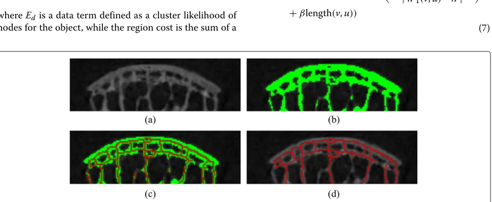
Fig. 9The skeletonisation process.aThe input image.bThe mask image resulting froma, where the foreground bone tissues are in green.c
where−→n1(v,u)represents the vector starting from node
vto node u, −→n is a normalized principle vector of the vertebra, length(v,u) denotes the length of the skeleton path betweenvandu, arccos(||−→n1(v,u)||×||−→n||
|−→n1(v,u)·−→n| )is the inter-section angle between vector−→n1and vector−→n, which is
among the range [ 0,π2], β is a weighting factor for bal-ancing the intersection angle and the length of edge. The design of the boundary term assign a higher weight to edge with shorter length and with direction similar to principle direction, which makes the minimal cut passes the edge standing for trabecula with such characteristic. With the help of the proposed graph cuts method, all the trabeculae between endplate and vertebra body can be found successfully.
2.4 Trabecula cutting
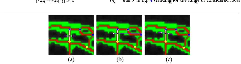
As a result, the graph cuts proposed above labeled the ver-texes into two sets, and the edges between the two sets stand for the trabeculae between the endplate and verte-bral body in our method; therefore, in order to obtain the final segmentation result, we have to further cut them. Our basic idea is to generate a proper straight line to achieve the purpose, while the main difficulty is the posi-tion and angle of the straight line. To solve the problem, an iterative searching strategy is proposed.
Firstly, we initialize a cut line described as a purple line in Fig.10a which passes through the trabecula represented by the white edge on the graph. The cut line locates at the middle of the white edge and forms two pointsp1andp2
when extending to the boundary of bone tissue (e.g., the white points in Fig.10). The distanced1between two ends
is|p1−p2|.
Next, we move the cut line towards the endplate at uni-form velocity. As the line moves, each move generates a updated two-ends distancedi(i=2, 3,· · · ·). When the cut line touches the endplate, thedi = |di−di−1|will
be increased dramatically. So we stop the movement when dimeet the Eq.8.
|di−di−1|> λ (8)
where we setλto 20 empirically.
Finally, the cut line will be rotated clockwise with a constant angle θ iteratively to get the proper angle. During each iteration, the distance di(j ∗ θ),(j = 1, 2,· · · ·, 2/θ) at the jth rotation will be compared withdi−1, namely,|di(j∗θ)−di−1|. The angle with
min-imal variation is the optmin-imal direction, which is the most parallel to the boundary of endplate, and the interface tra-becula can be cut completely according to such a line as described in Fig.10c.
3 Results and discussion
In this section, experiments designed to evaluate the per-formance of the proposed method will be presented. All experiments were carried out on a common personal computer with a Intel Core i3 processor (3.5 GHz) and 8 GB memory.
3.1 Experiment for shape prior extraction
In Section 2.2, we proposed two kinds of shape prior, which are the 3D gap line on the mesh surface and the 2D gap line within CT slices. Since the 3D gap line serves as the foundation of the 2D gap line detection, its extraction performance is firstly assessed.
3.1.1 Shape prior extraction results
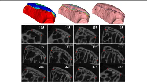
We test effect of the proposed shape prior extraction method by employing it for all vertebra in our data set. The (1) generated harmonic field, (2) isoline candidates and (3) resulting 3D gap line of a randomly selected verte-bra are shown in the first row of Fig.11from left to right respectively. Since the 3D gap line will be further trans-formed into two terminal points of the 2D gap line, Fig.11 also shows the corresponding terminal points (i.e., the red dots) within some typical slices, whose index are labeled on the top-right of the slice image. From the figures, we can see that both the 3D gap line and terminal points are correctly detected.
3.1.2 Parameter evaluation of 3D gap extraction
During the selection of the best isoline, there is a param-eterkin Eq.4standing for the range of considered local
Fig. 11Experimental results of shape priori extraction. The generated harmonic field, isoline candidates and the resulting 3D gap line of a randomly selected vertebra are shown in the first row from left to right respectively. The rest part shows the terminal points corresponding to the 3D gap line within some typical slices
region. As we mentioned, the extraction result is insensi-tive to the value ofk, and we set it to 6 empirically. In order to prove that, another experiment is carried out, where we vary the value ofkfor the optimal 2D gap line selection and check out for the differences.
Specifically, let Ga be the selected gap line when k equals toa, then we can have 7 gap lines under the con-ditions thatkvaries from 3 to 9 (i.e.,G3,G4,· · · ·,G9).
In order to see the differences between them, we calcu-late theDCD(Ga,G6),(a ∈[ 3, 9]a = 6) which is the
directional cut discrepancy (DCD) metric as employed in our previous work [16] to act as the mean errors comparing Ga with G6 in millimeters. We randomly
selected eight vertebra from the data set and extract eight gap lines for each of them. We calculate the
DCD data for these eight cases, and record them in Table1.
From the table, we can see that on the one hand, most of the DCD data are zero, which means we can have the same gap line withkvaries slightly for most of the cases. On the other hand, all non-zero data are very small, which means even if the selected gap line is different from the desired one under some circumstances, the mean errors between them is within a reasonable tolerance. In summary, the gap line extraction method is effective and efficient, the result is tolerable to the choice ofk.
3.2 Segmentation results
The next experiment is to test the effect of the proposed method by segmenting every vertebra in our data set. The
Table 1DCD records for evaluation ofKdefined in Eq.4
I II III IV V VI VII VIII
DCD(G3,G6) 0.02 0 0.14 0 0.04 0 0 0
DCD(G4,G6) 0 0 0.09 0 0.04 0 0 0
DCD(G5,G6) 0 0 0 0 0 0 0 0
DCD(G7,G6) 0 0 0 0 0 0 0 0
DCD(G8,G6) 0.02 0 0 0 0 0 0 0
Fig. 12The segmentation results in terms of 2D slices. The proposed method is employed to a randomly selected vertebra, the color regions of the 12 slices in the first, and second two rows are two endplates of the vertebra respectively
experimental results show that most of the endplates (93% exactly) can be successfully segmented, the reason for a few failed cases is mainly due to the great damage of the target vertebra.
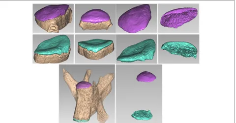
Among the successful ones, segmentation results of a randomly selected vertebra are shown in both 2D (Fig. 12) and 3D (Fig. 13). Figure 12 shows the seg-mentation results in terms of 2D slices. The first and
second double-row slices belong to the two endplates of selected vertebra respectively. The slices were uni-formly selected from different sagittal views. Figure 13 shows the segmentation results in terms of recon-structed 3D meshes, namely, the first and second row depict two endplates of the target vertebra in differ-ent perspective views, while the third row shows the relationship between the endplates and the rest parts of
Table 2Accuracy evaluation of the proposed segmentation method based on VD, Dice, ASSD, and MSSD metrics
Endplate Dice(%) ASSD(μm) MSSD(μm) VD(μm3)
L4U 91.02±1.8 2.77±0.01 7.85±0.13 79.23±8.9
L4D 90.43±3.2 3.09±0.06 6.96±0.27 84.79±11.2
L5U 91.14±2.6 2.48±0.03 8.11±0.32 76.51±9.6
L5D 90.88±2.7 4.02±0.02 7.55±0.19 82.14±10.5
the vertebra. From the figures, we can conclude that the endplates were successfully segmented using the proposed method.
3.3 Quantitative results
There are many approaches proposed for human’s ver-tebra segmentation; however, there is no study on mice endplate segmentation from micro-CT data except our study; therefore, no other methods can be found for comparison. Instead, we compared our results with the ground truth which are manually segmented by experi-enced experts with an image editing software slice-by-slice. In order to carry out the comparisons, four metrics are used to quantitatively evaluate the segmentation accu-racy, which include volume difference (VD, μm3), dice similarity coefficient (DC, %), and two surface distance metrics, i.e., average symmetric surface distance (ASSD,
μm), maximum symmetric surface distance (MSSD,μm) [26,27].
Table 2 shows the segmentation accuracy of the proposed method in terms of the metrics described above for the segmentation results mentioned in Section3.2. For better analysis, we classified the statistical results of end-plates according to their anatomical positions, namely, the L4U, L4B, L5U, and L5B stand for the upside/downside endplate of the fourth/fourth lumbar vertebra respec-tively. As shown in Table2, four types of endplate’s Dice coefficient are all more than 90%, the average DC is
91.33±2.8%. The average ASSD of the endplates is 3.02± 0.04μm, which is smaller than 4μm. L5U has the largest MSSD, which is less than 8.5μm.
As the VD data shows, the concave angle of upside end-plate is typically less than that of downside endend-plate within the same vertebra. For example, L4U with VD less than that of L4D. It can be interpreted by the fact that the surface of upside endplate is usually more flat than that of the downside one. In additional, endplate of L5 has higher Dice coefficient than the that of L4, which is mainly because, comparing with L4, L5 is closer to the ischium, and the concave angle of L5 is typically smaller in general. According to the results illustrated above, we can draw the conclusion that our method is accurate and complies with the actual anatomic shape feature of mice endplate.
3.4 Computational efficiency
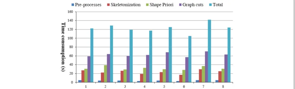
As another important issue, the efficiency of the proposed method can be assessed by system time consumptions. Therefore, time consumption for each process of the pro-posed method including the pre-process, skeletonization, shape priori and graph cuts, are recorded. Figure14shows 8 cases of our records. For each case, the input data contains 6 endplates represented by 610 slices in total.
According to Fig.14, the average time consumption for the pre-process, skeletonization, shape priori and graph cuts are 4.13±0.83 s, 24.63±4.27 s, 32.25±3.88 s, and 62.88± 4.42 s respectively. And it takes around 20 s to segment one endplate using the proposed method, which is approved by the doctors.
4 Conclusions and future work
In this paper, an intelligent framework is proposed to seg-ment each endplate from micro-CT data captured from the vertebral column of mice. The innovations of the pro-posed method can be summarized as the following three aspects. Firstly, this work is one of few researches which focus on endplate segmentation. Secondly, we solve the
endplate segmentation as a recognition problem of trabec-ulae within 2D gap area formed by target endplate and its adjacent vertebral body by a graph-based strategy. Thirdly, both 3D and 2D shape priori of the vertebra are used to guide for the segmentation, which are extracted by a harmonic field-based ranking method and a spline-fitting method respectively.
To assess the proposed method, experiments for shape prior extraction, accuracy and efficiency evaluation, and demonstrations of the segmentation results are presented and discussed in details, which proved the effective and efficiency of this work. However, there still have some works that could be done in the future including improve-ment of the accuracy and efficiency by incorporating more reliable shape priori and optimizing the graph cut-related procedures, since it consumes half of the total time as shown in the experiment.
Abbreviations
3D: Three-dimensional; ASSD: Average symmetric surface distance; CT: Computed tomography; DC: Dice similarity coefficient; DCD: Directional cut discrepancy; IVD: Intervertebral disc; MSSD: Maximum symmetric surface distance; ROI: Region of interest
Acknowledgements
The authors gratefully acknowledge the helpful comments and suggestions of the reviewers, which have improved the presentation.
Funding
This work is supported by the National Natural Science Foundation of China (61872085, 61772556), Scientific Research Project of Fujian University of Technology (GY-Z160130, GY-Z160138, GY-Z160066), the Natural Science Foundation of Fujian Province (2017J05098, 2017H0003, 2018Y3001), Project of Fujian Education Department Funds (JK2017029, JZ160461), Project of Fujian Provincial Education Bureau (JAT160328, JA15325) and Project of Science and Technology Development Center, Ministry of Education (2017A13025).
Availability of data and materials Please contact author for data requests.
Authors’ contributions
S-JL and ZZ contributed equally to the design and plan of the algorithm. ZZ collects all the materials and related literatures. S-JL offers feasible experimental scheme. JSP and S-HL offer the micro-CT data and guide the research. All authors read and approved the final manuscript.
Competing interests
The authors declare that they have no competing interests.
Publisher’s Note
Springer Nature remains neutral with regard to jurisdictional claims in published maps and institutional affiliations.
Author details
1Fujian Provincial Key Laboratory of Big Data Mining and Applications, Fujian University of Technology, No3 Xueyuan Road, University Town, Minhou, 350108 Fuzhou, China.2Colleague of Mathematics and Informatics, Fujian Normal University, Shang Street, Minhou district, 350117 Fuzhou, China. 3College of Computer Science and Engineering, Shandong University of Science and Technology, 266590 Qindao, China.4Department of Information Management, Chaoyang University of Technology, Taizhong, Taiwan.5School of Information Science and Engineering, Central South University, No.932 South Lushan Road, 410083 Changsha, China.
Received: 15 August 2018 Accepted: 29 March 2019
References
1. E. Perilli, I. H. Parkinson, L.-H. Truong, K. C. Chong, N. L. Fazzalari, O. L. Osti, Modic (endplate) changes in the lumbar spine: bone micro-architecture and remodelling. Eur. Spine J.24(9), 1926–1934 (2015)
2. M. Muller-Gerbl, S. Weiber, U. Linsenmeier, The distribution of mineral density in the cervical vertebral endplates. Eur. Spine J. Off. Publ. Eur. Spine Soc. Eur. Spinal Deformity Soc. Eur. Sect Cervical Spine Res. Soc. 17(3), 432–438 (2008)
3. S. Brown, S. Rodrigues, C. Sharp, K. Wade, N. Broom, I. W. McCall, S. Roberts, Staying connected: structural integration at the intervertebral disc-vertebra interface of human lumbar spines. Eur. Spine J.26(1), 248–258 (2017)
4. N. Newell, C. A. Grant, M. T. Izatt, J. P. Little, M. J. Pearcy, C. J. Adam, A semi-automatic method to identify vertebral end plate lesions (Schmorl’s nodes). Spine J.15(7), 1665–1673 (2015)
5. J. S. Athertya, G. Saravana Kumar, Automatic segmentation of vertebral contours from CT images using fuzzy corners. Comput. Biol. Med.72, 75–89 (2016)
6. E. Cheng, Y. Liu, H. Wibowo, L. Rai, in2016 IEEE 13th International Symposium on Biomedical Imaging (ISBI). Learning-based spine vertebra localization and segmentation in 3D CT image, (2016)
7. R. Korez, B. Ibragimov, B. Likar, F. Pernuš, T. Vrtovec, A framework for automated spine and vertebrae interpolation-based detection and model-based segmentation. IEEE Trans. Med. Imaging.34(8), 1649–1662 (2015)
8. M. Pereañez, K. Lekadir, I. Castro-Mateos, J. M. Pozo, Á. Lazáry, A. F. Frangi, Accurate segmentation of vertebral bodies and processes using statistical shape decomposition and conditional models. IEEE Trans. Med. Imaging. 34(8), 1627–1639 (2015)
9. Y. Kim, D. Kim, A fully automatic vertebra segmentation method using 3D deformable fences. Comput. Med. Imaging Graph.33(5), 343–352 (2009) 10. Q. Wang, L. Lu, D. Wu, N. Y. El-Zehiry, Y. Zheng, D. Shen, S. K. Zhou,
Automatic segmentation of spinal canals in CT images via iterative topology refinement. IEEE Trans. Med. Imaging.34(8), 1694–1704 (2015) 11. C. Yen, H.-R. Su, S.-H. Lai, inPattern Recognition (ACPR), 2013 2nd IAPR Asian
Conference On. Reconstruction of 3D Vertebrae and Spinal Cord Models from CT and STIR-MRI Images (IEEE, Naha, 2013), pp. 150–154.https://doi. org/10.1109/ACPR.2013.32
12. K. Zhao, Z. Q. Wang, Y. Kang, H. Zhao, A highly automatic lumbar vertebrae segmentation method using 3D CT data. J. Northeast. Univ. 32(3), 340–317 (2011)
13. L. Li, H. Cai, Y. Zhang, W. Lin, A. Kot, X. Sun, Sparse representation based image quality index with adaptive sub-dictionaries. IEEE Trans. Image Process.25(8), 3775–3786 (2016)
14. L. Li, Z. Yu, G. Ke, W. Lin, S. Wang, Quality assessment of dibr-synthesized images by measuring local geometric distortions and global sharpness. IEEE Trans. Multimedia.PP(99), 1–1 (2017)
15. S. Liu, Y. Xie, A. P. Reeves, Automated 3D closed surface segmentation: application to vertebral body segmentation in CT images. Int. J. Comput. Assist. Radiol. Surg.11(5), 789–801 (2016)
16. B. J. Zou, S. J. Liu, S. H. Liao, X. Ding, Y. Liang, Interactive tooth partition of dental mesh base on tooth-target harmonic field. Comput. Biol. Med.56, 132–144 (2015)
17. S. H. Liao, S. J. Liu, B. J. Zou, X. Ding, Y. Liang, J. H. Huang, Automatic tooth segmentation of dental mesh based on harmonic fields. BioMed Res. Int. 2015, 1–10 (2015)
18. G. Buttazzo, G. Dal Maso, Shape optimization for Dirichlet problems: relaxed formulation and optimality conditions. Appl. Math. Optim.23(1), 17–49 (1991)
19. Y. Boykov, M. P. Jolly, inMICCAI 2000: Proceedings of the Third International Conference on Medical Image Computing and Computer-Assisted Intervention, ed. by S. L. Delp, A. M. DiGoia, and B. Jaramaz. Interactive organ segmentation using graph cuts (Springer, Berlin, 2000), pp. 276–286.https://doi.org/10.1007/978-3-540-40899-4_28 20. A. Delong, Y. Boykov, in2009 IEEE 12th International Conference on
Computer Vision. Globally optimal segmentation of multi-region objects (IEEE, Kyoto, 2009).https://doi.org/10.1109/ICCV.2009.5459263 21. M. G. Linguraru, W. J. Richbourg, J. F. Liu, J. M. Watt, V. Pamulapati, S. J.
22. D. Mahapatra, Combining multiple expert annotations using semi-supervised learning and graph cuts for medical image segmentation. Comput. Vis. Image Underst.151, 114–123 (2016) 23. Y. Pauchard, T. Fitze, D. Browarnik, A. Eskandari, I. Pauchard, W. Enns-Bray,
H. Pálsson, S. Sigurdsson, S. J. Ferguson, T. B. Harris, V. Gudnason, B. Helgason, Interactive graph-cut segmentation for fast creation of finite element models from clinical ct data for hip fracture prediction. Comput. Methods Biomech. Biomed. Eng.19(16), 1693–1703 (2016)
24. R. Cardenes, J. M. Pozo, H. Bogunovic, I. Larrabide, A. F. Frangi, Automatic aneurysm neck detection using surface voronoi diagrams. IEEE Trans. Med. Imaging.30(10), 1863–1876 (2011)
25. G. D. Li, X. J. Chen, F. Shi, W. F. Zhu, J. Tian, D. H. Xiang, Automatic liver segmentation based on shape constraints and deformable graph cut in CT images. IEEE Trans. Image Process.24(12), 5315–5329 (2015) 26. Y. Gan, Z. Xia, J. Xiong, Q. Zhao, Y. Hu, J. Zhang, Toward accurate tooth
segmentation from computed tomography images using a hybrid level set model. Med. Phys.42(1), 14–27 (2014)