Optimization of triple inverted pendulum control process based on motion vision

R E S E A R C H

Open Access

Optimization of triple inverted pendulum

control process based on motion vision

Xiaoping Huang

, Fangyi Wen

and Zhongxin Wei

Abstract

An inverted pendulum is a typical nonlinear and absolutely unstable system. In order to control the triple inverted pendulum effectively and steadily, an optimization method of inverted pendulum control process based on motion vision was proposed. The real-time motion pictures of the triple inverted pendulum in the swinging-up process were collected through the CCD camera, and the real-time motion pictures of the triple inverted pendulum were recognized, matched and optimized by using Harris algorithm. By using motion vision to control and optimize the triple inverted pendulum, the stabilization control of the triple inverted pendulum was realized.

Keywords: Motion vision, Triple inverted pendulum, Control process optimization

1 Introduction

The inverted pendulum is the model of the most bal-anced control and the lack of driving control system, which is widely used in teaching and theoretical re-search. Therefore, for many years, people have been working on the problem of inverted pendulum control in theory and function. The theory of control operation and the method of control will have a great promotion and positive significance for the industrial production. Automatic control is a highly theoretical subject and it is a very important engineering technology. The engin-eering technology theory mentioned in the literature [1] was “automatic control theory.” In the scope of the improvement of the control theory, it is not feasible to use the theory in reality without proving the correct-ness of a theory. It is necessary to design the controller according to its theory in order to achieve the true value of the theory [2, 3]. In literature [4], it was pointed out that the inverted pendulum, as a target of experiment, is a system with multiple variables, rapid transformation, nonlinearity, and poor stability. We can add a control algorithm to increase its stability to prove the processing ability of the control method for com-plex, unstable, and nonlinear systems. At the same

time, how this method embodies the difficult problems in a series of automatic control categories, such as ro-bustness, stabilization, and tracking in the process of controlling the system, could also be reflected in the process of controlling the inverted pendulum move-ment. Therefore, it was concerned by the scientists. Using different control algorithms, different types of inverted pendulum control have become a worldwide research topic with high research value [5,6].

The fuzzy control theory was used to control the inverted pendulum in the literature [7], when the fuzzy control method was used to analyze the inverted pendulum problems, the mathematical theory was not used to analyze the nonlinear factors in the inverted pendulum system and the influence of them on the controller, but was used to analyze all kinds of unstable conditions caused by the method in the trol of the inverted pendulum, according to the con-troller’s experience and the previous experience. Finally, the mode of the fuzzy control theory set was used to express the processing methods. However, the fuzzy control theory did not have a concise and prac-tical way to deal with multivariable problems. There-fore, the analysis of the triple inverted pendulum system was not entirely applicable.

The neural network was applied to the inverted pendulum control system and developed rapidly in the early 1990s. It was mentioned in the literature * Correspondence:[email protected];[email protected];

[email protected]

1_{College of Mechanical and Electrical Engineering, Nanning University, No.8} Lonting Road, Nannin 530200, China

Full list of author information is available at the end of the article

[8] that the neural network could arbitrarily ap-proach the complex nonlinear relationship as much as possible, could learn to train data samples and was suitable for the absolutely unstable inverted pen-dulum control system, and could use the characteris-tics that all the characteristic information with a certain quantity or a certain nature could be evenly stored in each layer of neurons in the network, so this method had strong robustness and capacity. The back-propagation neural network could also be com-bined with the Q learning algorithm, and was used as the non-discrete model to control learning of inverted pendulum. However, due to the sensitivity of the neural network system and slow convergence rate, the computation of objective function was very complex and time consuming.

In view of the incomplete research of the inverted pen-dulum control system by the above methods, the triple inverted pendulum control system based on visual differ-ence feedback was proposed. The vision sensor camera was used to collect the image information during the inverted pendulum motion, and the image corner matching was applied to monitor the inverted pendulum in real time. Then, the mathematical model of the triple inverted pendulum control system was constructed, and the balance control of the inverted pendulum system was carried out through the linear quadratic optimal control theory [9,10].

2 Methods—optimization of triple inverted pendulum system control process

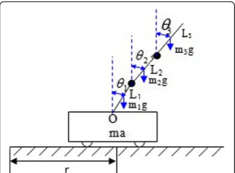
2.1 Inverted pendulum control system of motion vision After collecting the motion image information of triple inverted pendulum by visual sensor, we set up an application network remote control platform. The triple inverted pendulum was mainly composed of car, pendulum 1, pendulum 2, and pendulum 3, and there were free links between them. The car could move horizontally on the horizontal guide rail, and the pendulum bar could move freely in the vertical plane. The motion analysis of the system diagram was shown in Fig. 1.

Firstly, we used a camera to collect image information of inverted pendulum and make the image preprocess-ing. Then, we selected the annotation template and placed it in the same plane, collected the template im-ages from different angles, detected the feature points (corner points) in the image, obtained the internal and external parameters of the camera, and optimized the refinement.

Secondly, we extracted the image feature point in-formation. The corner detection method was based on Harris corner monitoring and matching method.

For the pixels (x,y) on the image, the image window

W (W(x,y) was the image window function) should be moved on the quantification (u,v). If we wanted to define the energy function E, the formula (1) was shown as follows.

E uð ;vÞ ¼X x;y

W xð ;yÞ½I xð þu;yþvÞ−I xð ;yÞ2 ð1Þ

The Harris corner was based on the grayscale images, soI(x,y) was represented the gray value of images. Taylor expansion method was applied to deal with small quan-tities, so when (u,v) was small,Ecould be represented by the following formula (2).

E uð ;vÞ≈½u;vM u

v ð2Þ

Among formula (3),

M¼X

x;y

W xð ;yÞ I

2

x IxIy IxIy I2y

¼

X

x;y GI2x

X

x;y

GIxIy

X

x;y

GIxIy

X

x;y GI2y

2 6 6 4

3 7 7 5

ð3Þ

Ix¼∂_∂I_x and Iy ¼∂_∂I_y respectively represented the first-order differential step degree of the image in the direction of x and y. The image had noise when it was obtained and conveyed, so there were many methods to increase the level of noise resistance. Gauss smoothing filter for anti-noise processing was used in this paper, andWwas the Gauss template function. The expression was shown in formula (4).

W xð ;yÞ ¼G¼ exp − 1 2σ2 x

2_þ

y2

ð4Þ

E was close to local autocorrelation function. As-suming that λ1 and λ2 were the eigenvalues of matrix M, we could use λ1 and λ2 to determine the corner.

R was defined as the interest value of the correspond-ing pixel points; the formula was shown as follows in formula (5).

R¼ det M−kðtraceMÞ2 ð5Þ

Among them, k was the constant, and according to the experience, the value was 0.04–0.06, trace M =λ1 +λ2 represented the direct trace of the matrix, and det M =λ1λ2 was the determinant of the matrix. Then, the basis for obtaining Harris corner was that the_Rvalue of a pixel in a frame was the best in other areas, which was greater than the set thresholdR0.

There was a phenomenon of rotation and deviation in the two images. Under the condition of obtaining the corner with the same threshold R0, if the corner set of

the overlapping parts of the image was set to_Aand A′, the necessary condition for the image matching was given first:

1. The number of corners should be the same,A

= {a1,a2,…,an} andA′= {a1′,a2′,…,an′}had the same number of corners;

2. a1anda1′were the corresponding corners, then they had the same corner valueR(a1) =r(a1′); 3. Ifa1anda1′were the corresponding corner points,

their number of adjacent corner points should be equal, that wasNr(a1) =Nr(a1′),rrepresented the neighborhood radius;

4. If {a1,ai}εA, {a1′,ai′}εAwere the corresponding corner point, then their distance was equal d(a1,ai)

=d(a1′,ai′);

5. Ifaiandajwere corresponding corner points,ai′

andaj′were other corresponding corner points, {a1,ai}εA, {a1′,ai′}εA. According toai,aj,ai′, and

aj′, the matching parameter was calculated by the following formula (6).

Pij¼ Δxij;Δyij;Δθij

ð6Þ

△xij and △yij were the translational quantities of the

image waiting for matching for the matching image onx

and y axis,△Ѳijwas the angle of rotation. If the

match-ing parameter Pijof any matching corner point in theA

and A′set was the constant vector, then the two images matched completely.

2.2 Motion control optimization of triple inverted pendulum system

Firstly, we constructed the mathematical model of triple inverted pendulum system according to La-grange equation and set r as the motion displacement of horizontal guide rail, and Ѳ1, Ѳ2, and Ѳ3 were

re-spectively the angles of the lower, middle, and upper pendulums relative to the vertical direction. The La-grange equation for the triple inverted pendulum sys-tem with conservative force and dissipative force were shown in the following formula (7).

d dt

∂T

∂q_i

−∂_∂T_{_}

qi þ∂_∂V

qi þ_∂∂D_{_}

qi

¼ Fqi ð7Þ

In the formula,qirepresented the generalized

coordin-ate, that were r, Ѳ1, Ѳ2, Ѳ3; Fqi was the non-potential

generalized force, when qi=r, Fqi=G0U,U was the

con-trolled quantity, G0and was the gain constant. Whenqi

=Ѳ1,Ѳ2, andѲ3,Fqi= 0,T,V, andDwere respectively the

function, potential energy, and dissipative energy of the

system, then T ¼P

i¼0 n

Ti, V ¼ P i¼0

n

Vi, and D¼ P i¼0 n

Di. Among them, n was the stage number of the inverted pendulum(n= 3); Ti,Vi, andVi were kinetic energy,

po-tential energy, and dissipative energy of cars and all levels of pendulum. The mathematical model could be obtained by putting Ti,Vi and Di(i= 0, 1, 2, 3) into the

formula (8).

Mðθ1;θ2;θ3Þ rn θ1n θ2n θ3n 2 6 6 4 3 7 7

5þN θ1;θ2;θ3;θ1_ ;θ2_ ;θ3_

r0 θ10 θ20 θ30 2 6 6 4 3 7 7

5¼G uð ;θ1;θ2;θ3Þ

ð8Þ

Formula (8) was a nonlinear vector differential equation. When the system worked, it moved on the edge of the equilibrium position. In the formula, when u= 0, it was linearized near the equilibrium positionr¼θ1¼θ2¼θ3

¼r_¼θ_1¼θ_2¼θ_3¼0 instead of the nonlinear vector

differential equation.

Secondly, a linear quadratic optimal control was in-troduced to improve the triple inverted pendulum system.

1. The pendulum bars were linked by hinges without any constraints, so it was difficult to control the attitude in the initial swing.

of the triple inverted pendulum in the initial swing process, we used the finite-time time in-variant LQ (liner quadratic) problem to achieve the optimal control.

−P t_ð Þ ¼P tð ÞAþATP tð Þ þQ tð Þ

−P tð ÞBR−1ð ÞBt TP tð Þ P tf ¼S;t∈ t0;tf

8 <

: ð9Þ

In the formula (9), A and B were the coefficient matrices of the corresponding dimensions, S was the weighting matrix, and t was the adjusting time. The solution matrix P(t) was n×n positive semi definite symmetric matrix, then the necessary and sufficient conditions of the optimal control u_ð•Þ were shown in formula (10).

_

u tð Þ ¼−K t_ð Þ_x tð Þ;K t_ð Þ ¼R−1BP tð Þ ð10Þ

The optimal trajectoryx_ð•Þwas shown in formula(11).

_

x tð Þ ¼A_x tð Þ þBu t_ð Þ;x t_ð Þ ¼0 x0 ð11Þ

The optimum performance value_J ¼ Jðu_ð•ÞÞwas shown in formula (12).

_ J ¼1

2x

T

0P tð Þx0 0;∀x0≠0 ð12Þ

The optimal control system was adjusted by finite-time time invariant LQ, and its control state was observed. The feedback was that the inverted pendulum was stabilized and the jitter time was short in the process from swinging up to steady state.

2. The other key link of the triple pendulum automatic swing was the stable state entering the inverted position after swinging up. This area was a balance control problem. If it could not be effectively controlled, it would lead to the failure of the whole control system. Therefore, the control tending to steady state was based on the infinite-time LQ to adjust the optimal control. The sufficient and necessary condition for the given infinite-time time invariant LQ to regulate optimal control was shown as follows in formula (13).

_

u tð Þ ¼−K t_ð Þ_x tð Þ;K_ ¼R−1BT_{P ð13Þ}

The equation of state for the optimal trajectory x_ðtÞ

was shown in formula (14).

_

x tð Þ ¼A_x tð Þ þBu;x_ð Þ ¼0 x0 ð14Þ

The optimal performance value _J ¼ Jðu_ð•ÞÞ was shown in formula (15).

_

J ¼xT0Px0;∀x0≠0 ð15Þ

3. Two-point boundary value problem: The triple pendulum control system was in the limited

time t∈[0,T], and the following boundary value

conditions was satisfied to the process from static sag to vertical inverted position.

y tð Þt¼0;T¼0;y_ð Þt _t¼0;T¼0 ð16Þ

θð Þ ¼0 ½π π πT;θ_ð Þt _t¼0;T¼0 ð17Þ

Among them,t= 0 was the initial value condition, and

t= T was the final value condition. In addition, accord-ing to the performance of the hardware, and the high sensitivity and strong instability of the triple pendulum control system, the action of the car must also satisfy the following constraints during the hoisting process.

y

j j≤1:5m;j jy_ ≤5m=s;j j€y ≤20m=s2 ð18Þ

θ¼ ½θ θ_Τ¼ ½θ1 θ2 θ3 θ_ 1 θ_

2 θ_

3was appointed, the first-order ordinary differential equations could be ob-tained was shown in formula (19).

_

θ¼β θ_{;θ_;€}

y

¼ θ

1 θ2 θ3 θ_ 1 θ_

2 θ_

3

h i

ð19Þ

Where the vector function β¼ ½β₁ β₂ β₃ β₄ β₅ β₆Τ, the edge value condition were shown in formula (19) and formula (20).

θ_{ð Þ ¼0 ½π π π}T_;θ_ 0

ð Þ ¼0 ð20Þ

θ_{ð Þ ¼T 0;θ_}

T

ð Þ ¼0 ð21Þ

Obviously, ordinary differential Eq. (19) and boundary value condition (20), (21) were formed a nonlinear two-point boundary value problem.

4. Reference ground track: The design method of the nominal trajectoryy* =γ(t,p) was not unique, polynomial functions or cosine series could be selected. In general, the inputu*(t) was required to be continuous, soγ(t,p) must meet the demands of quadratic differential ifα= 2.

We should combine the finite-time and infinite-time invariant LQ regulation to improve the control, so that the system could reduce the attitude adjustment time in the automatic swing-up transition process and could quickly enter the stable stage of the automatic swinging up. After entering the stable stage, the inverted control of the triple pendulum was also the key stage. Through the adjustment of the infinite-time time invariant LQ, the system would maintain a steady and gradual process in a state tending to equilibrium.

3 Analysis of the result of optimization process

The inverted pendulum system was a very unstable sys-tem. In order to stabilize the state of the automatic swing-up transition stage and steady swing phase during

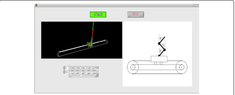
the control process, the finite-time and infinite-time in-variant LQ were used to adjust the optimal control to im-prove the triple inverted pendulum system in this paper. In order to prove the effectiveness of the improved method in the aspect of stability control, we carried out experiments in MATLAB simulation environment, and waw collected datum and analyzed them. In the process of control, the moving effect of the pendulum and car in the triple inverted pendulum was presented visually and viv-idly in the form of animation in Fig.2. And we could ob-serve that many directions control the motion of the rocker and the car in the process of the controller to con-trol the whole process of mobile, and it was a very vivid triple inverted pendulum visual simulation platform.

4 Results and discussions 4.1 Experiment 1

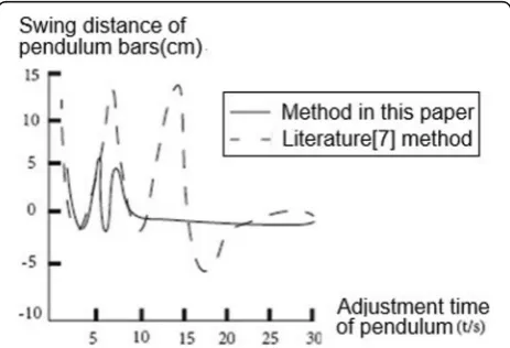
In automatic swing-up transition phase, in order to con-trol the accurate swing of cars and pendulum bars, the finite-time time invariant LQ was used to adjust the opti-mal control, then we could achieve the steady state of the pendulum bars in the initial swing process, after the sys-tem was adjusted by the method in the text and literature [7] method, they gradually reached a stable state. The fol-lowing table was the control time data of automatic swing-up adjustment when the pendulum bars by two methods starts to swing was shown in Table1.

Fig. 3Comparison of adjustment time curves of pendulum bars of two methods.

Table 1The automatic swing-up adjustment control schedule

Methods Moving distance of pendulum (cm)

Adjustment time (t/s)

Method is this paper 15 7

From data analysis of Table 1, the two methods ad-just the initial swing stage of the inverted pendulum simultaneously. It could be seen from the data that the adjustment time of the literature [7] method was too long, so the stability of the control system was not strong. According to Table 1, we could get the adjustment time curve figure of the inverted pendu-lum of two methods, as shown in Fig. 3.

From the two curves of Fig.3, it was observed that the time consuming of the inverted pendulum from the ini-tial pendulum to the steady motion of the pendulum bar was about 7–8 s, while the time consuming of the litera-ture [7] was about 25 s. Therefore, the control perform-ance of the initial pendulum stage of the method in this paper was better.

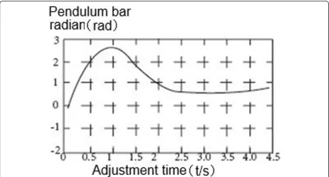
In the process of inverted pendulum adjustment, the swing angle radian would be generated. From Figs.3to4, we would analyze the swing angle radian in the initial swing time of the inverted pendulum controlled by two methods.

From Figs.4 and5, we could see the difference of the swing radian in the swinging-up stage of the inverted pendulum. After using the method in this paper to con-trol the inverted pendulum, the swing angle radian of initial swing was much less than that of literature [7] method, and it was indicated that the method in this paper was effective for the triple inverted pendulum in the initial swing stage.

4.2 Experiment 2

Stable swing stage: For the stable swing stage of the triple inverted pendulum from initial swing stage to the steady motion, the swing state was the control of the balance. Figure 6 was the comparison of the optimal control curve given by the system and the curves of the steady swing stage of two methods.

The motion velocity of inverted pendulum in steady swing stage could be analyzed from Fig. 6, the motion

Fig. 5The radian adjustment figure of the inverted pendulum by the method in this paper.

velocity of the inverted pendulum controlled by the method in this paper was close to the optimal speed of the system, and the goodness of fit was better. The mo-tion speed of literature [7] algorithm was faster, and it was indicated that the inverted pendulum was always in a state of quivering.

4.3 Experiment 3

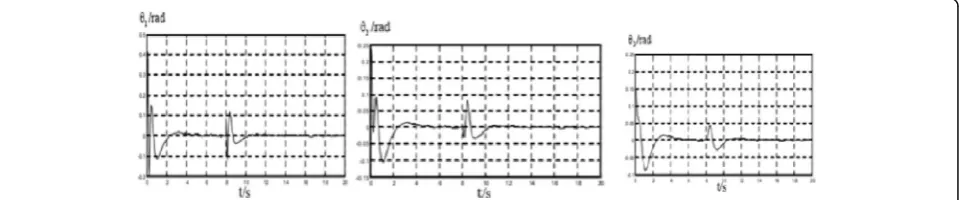
When we constructed the triple inverted pendulum con-trol model, at first, we set an initial displacement angle for triple inverted pendulum, and the starting position of the three-stage inverted pendulum car was given by the simulation control system to the force F in a uniform direction at the bottom of the car. Within 20 s, we re-corded the motion state and the degree of pendulum and kept the car in a set of orbit range (0 to 10 m), then kept the third movement that did not exceed the scope of the above a predetermined angle.

The initial object of the three-stage inverted pendu-lum system was set in the same range and randomly selected in the above range. Through constant up-dates, the control system could control the inverted pendulum, so the time of its movement was within the prescribed limits. The time period and sampling frequency were 0.5 s to ensure that the three-stage

inverted pendulum could be maintained in a certain angle. In the case of white noise signal interference and shock signal interference, the stability of the sys-tem was maintained, and the robustness was strong. The range and control of the upper, middle and lower positions with white noise and impulse were shown in Fig. 7a–c.

With the control method of this paper, the ampli-tude of the three-stage inverted pendulum could be stabilized at a certain time. This method had the ad-vantages of high modeling accuracy and good control-lability, which could be used to solve the problems of complex systems which were difficult to solve by trad-itional methods.

5 Conclusions

In this paper, the triple inverted pendulum control system based on the motion vision was proposed, and motion at-titude of the inverted pendulum was monitored by vision sensor. The finite-time and infinite-time time invariant LQ control method were introduced to control the bal-ance of the triple inverted pendulum from the initial swing stage to the steady swing stage. The experiments showed that the inverted pendulum control system designed in this paper solved the problem of changeable and unstable

Fig. 7The control curve of the triple inverted pendulum

inverted pendulum. The parameters of the controller were further optimized on the basis of optimizing feedback control parameters; thus, we could improve the conver-gence speed of the system. The design of the controller ac-cords with the goal and principle of triple inverted pendulum control system, which was an effective design scheme, and it could provide some reference value for other fields of the control theory.

Abbreviations

CCD:Charge coupled device; LQ: Liner quadratic

Acknowledgements

The authors thank the editor and anonymous reviewers for their helpful comments and valuable suggestions.

Funding

This work was supported in part by a grant from the Industry-Academy Cooperation Education Project of the Ministry of Education (project No.201702135097), the Science and Technology Planning Project of Guangxi Bureau of quality and technology supervision (contract No.GXKJJH2018009).

Availability of data and materials

The data and materials are available from the corresponding author on reasonable request.

Authors_’contributions

All authors have taken part in the discussion of the work described in this paper. XH wrote the first version of the paper. FW took part in the experiments of the paper. ZW revised the paper in different versions. All authors read and approved the final manuscript.

Authors_’information

Xiaoping Huang received the B.S. degree in automation from Hunan Industry University, Zhuzhou, China, in 1996, and the M.S. degree in Control Science and Engineering from Guilin University of Technology, Guilin, China, in 2007. From 1996 to 2010, he was a Senior engineer in Guilin Shuguang Rubber Industry Research and Design Institute. From 2011 to 2016, he was an associate professor of the college of Mechanical and Electrical Engineering at Nanning University. From 2017 to now, he was a professor of the college of Mechanical and Electrical Engineering at the same University. His research interests include Intelligent Control and Embedded System.

Fangyi Wen received her B.S. degree in Computer science and technology in Guilin University of Electronic Science and Technology in 2005, and she is currently a senior engineer at Guangxi Quality Technical Engineering School. Her current research interests focus on Computer Control Technology. Zhongxin Wei received his B. S. and M. S. degrees from Xi’an Jiaotong University in 1988 and 1991, he is currently engineer Senior engineer at Guangxi Quality Technical Engineering School. His current research interests include automatic detection technology.

Ethics approval and consent to participate Not applicable

Consent for publication Not applicable

Competing interests

The authors declare that they have no competing interests. And all authors have seen the manuscript and approved to submit to your journal. We confirm that the content of the manuscript has not been published or submitted for publication elsewhere.

Publisher’s Note

Springer Nature remains neutral with regard to jurisdictional claims in published maps and institutional affiliations.

Author details

1_{College of Mechanical and Electrical Engineering, Nanning University, No.8} Lonting Road, Nannin 530200, China.2_{Guangxi Quality Technical Engineering} School, No.8 Lonting Road, Nannin 530200, China.

Received: 16 April 2018 Accepted: 25 June 2018

References

1. A Guo, H Zhou, Teaching reform for automatic control principle. J Electr Electron Educ36(1), 11–12 (2014)

2. Y Liu, P Wang, L Liao, et al., LOR controller optimization for double inverted pendulum based on improved artificial bee colony algorithm. Comput Measur Control22(9), 2820_–2822 (2014)

3. X Wang, W Chen, X Zhao, Overview of swing-up and stability control of the inverted pendulum system. Tech Autom Appl34(11), 5–9 (2015)

4. Q Wang, H Huang, Symbol-type adaptive fuzzy control on inverted pendulum system. Commun Eng Des35(3), 1016_–1020 (2014) 5. Z Zhang, X Wei, S Wang, Study and design of the rotational inverted

pendulum based on 52 microcontroller. J Langfang Teach Coll14(4), 49–52 (2014)

6. Z Wu, Real-time simulation of control system based on RTX, Simulink and LabWindows/CVI. Electron Des. Eng22(13), 44–47 (2014)

7. Q Song, D Li, The design and stability study of double inverted pendulum controller. Comput Simul32(4), 305–309 (2015)

8. S Zhu, X Wang, W Liu, Robust adaptive repetitive control for periodically time-varying systems. Acta Automat Sin40(11), 2391–2403 (2014) 9. D Qiao, Y Zhang, L Shi, Optimization design of binocular stereo vision

sensor based on genetic algorithm. Journal of Natural Science of Hunan Normal University37(6), 53_–56 (2014)