Some considerations in heterogeneous nonisothermal transport models for wood: a numerical study

ORIGINAL ARTICLE

Wook Kang · Woo Yang Chung · Chang-Deuk Eom Hwanmyeong Yeo

Some considerations in heterogeneous nonisothermal transport models for

wood: a numerical study

Abstract This study compares a number of coupled heat and mass transfer models and presents numerical compari-sons of phenomenological coeffi cients between the four models (Stanish, Perre, Pang, and Avramidis) that are most frequently used in the literature to describe wood-drying processes. The USDA sorption isotherm, the Hailwood-Horrobin model, was adopted to calculate the relations between moisture content in wood and water vapor pressure at any temperature. Due to different assumptions about the driving forces of heat and mass transfer, coeffi cients in each model represent different values for moisture content and temperature and are closely related to each other. In the case of isothermal mass transfer, the moisture diffusion coeffi cient in the transverse directions from the Stanish and Pang models increased with decreasing moisture content. This contradicts the Avramidis and Perre models and numer-ous experimental results. Thermal diffusion effects on the drying process may not be predominant because the noniso-thermal state is relatively short. Therefore, the Perre model, which does not consider the thermal diffusion effect, has been used successfully in the drying simulation. However, it may be erroneous in certain cases when the nonisothermal state prevails over the system, such as building physics. The Pang model cannot explain the phenomena of thermal dif-fusion and moisture thermodifdif-fusion. It might be reasonable to modify the thermal diffusion of the Avramidis model, which is lower than that of the Stanish model. The apparent heat diffusivity was higher than the true heat diffusivity.

Key words Nonisothermal transport model · Drying · Build-ing physics · Phenomenological coeffi cients · Sorption isotherm

W. Kang · W.Y. Chung

Division of Forest Resources and Landscape Architecture, Chonnam National University, Gwangju 561-756, Republic of Korea

C.-D. Eom · H. Yeo (*)

Department of Forest Sciences, Research Institute for Agriculture and Life Sciences, Seoul National University, San 56-1, Sillim-dong, Gwanak-gu, Seoul 151-921, Republic of Korea

Tel. +82-2-880-4781; Fax +82-2-873-2318 e-mail: [email protected]

Introduction

Heat and mass transfer modeling is important for improving our knowledge of many engineering problems, such as the moisture-buffering capacity of wood in building physics,1 wood drying, and wood-based panel manufacturing during hot pressing. Most of the sophisticated models have been developed within the wood-drying research fi eld. Their importance is increasing because of the demand for wood components as building materials is expected to increase in the future and given that well-designed drying process control is required at present.

Moisture in wood exists in three phases: water vapor, bound water, and free water above the fi ber saturation point (FSP). There are two phases of water vapor in the cell cavities and bound water in the cell walls, below FSP in the hygroscopic range. The maximum bound water content is at the FSP and is limited by the number of sorption sites available. This may differ among species because their chemical compositions vary, but it is usually assumed that FSP is 30% water, based on the wood’s dry weight at room temperature.

It is well documented that the driving potential for the movement of free water and water vapor is the gradient of capillary pressure and vapor pressure, respectively. Fur-thermore, the fl ux of water vapor can be divided into the convection component of the gas mixture fl ux and the dif-fusion component of water vapor under the effect of a gra-dient in vapor concentration. However, the driving potential for the bound water differs according to researchers, and can be expressed in terms of a number of different system variables. Siau2

stated that under isothermal conditions it does not matter which potential is used in the diffusion equation as long as the appropriate diffusion coeffi cient is used. The most commonly used potentials are based on the chemical potential and the gradient of bound water concentration.

Under nonisothermal conditions, thermally induced mass transfer (thermal diffusion or Soret effect) should be taken into account in models. This is because there might

be a signifi cant temperature difference between the outer and inner surfaces of a building envelope, although this may be neglected in wood drying because the temperature change duration is relatively small.

In the literature, we can fi nd three distinct formulations of nonisothermal transport models that are widely accepted in wood drying and other research fi elds. First, Avramidis et al.3

developed Luikov-type equations mainly for model-ing wood drymodel-ing at low temperatures, and are based on a series of studies by Stamm,4

Choong,5

and Siau.2,6

Avramidis assumed that mass transfer is driven by moisture and tem-perature gradients. He used the combined bound water diffusion coeffi cient that involves both bound water and water vapor movement. However, the model can be applied only below the hygroscopic range and at low temperature below the boiling point of water because he did not consider capillary movement above the hygroscopic range and water vapor convection after change of water state to vapor. Second, Perre’s model7

is based on Whitaker’s multiphase transfer model8

with an additional potential of bound water. Perre et al.7

focused on heat and mass transfer modeling above the boiling point of water, in which mass transfer by gas convection is dominant. The bound water diffusion coeffi cient is based on Stamm’s result,4

which is similar to the Avramidis model. Third, Stanish9

assumed that bound water diffusion is driven by the chemical potential, which makes his model different from Perre’s model. It should be noted that both Stanish and Perre developed general models for nonhygroscopic as well as hygroscopic materials. Pang10 focused mainly on high-temperature wood drying and he used the driving potential for bound water similar to the chemical potential of Stanish’s model.

All the above models were compared for their ability to predict experimental results. Satisfactory agreements were obtained over given material and environmental conditions. However, not all the physical and transport coeffi cients were determined experimentally, and the validity would be uncontestable. The application of a model to various wood species might be questionable under a wide range of dynamic external conditions.

Kamke and Vanek11

compared the capacities of 12 wood-drying models with the experimental wood-drying results of mois-ture change rate and distribution that included the above three models (Avramidis, Perre, and Stanish). They stated that “none of the models violated any of the known wood-drying phenomena, but there was a high variability between

models’ results that was not in close agreement with the test runs. It might be due to uncertain coeffi cients for the models, different degrees of simplifi cations, and different ways of solving the heat and mass transfer equations.” In addition, the equations for boundary conditions and external heat and mass convection coeffi cients are usually different among models, which might affect the numerical results. Yeo and Smith12

developed the convective mass transfer coeffi cient conversion method, which proves that boundary-layer theory is useful for evaluating external moisture resistance during wood drying, using surface moisture data.

However, little work has been done on the numerical comparison of governing equations for heat and mass trans-fer models in wood because their assumptions and equation forms are different, and it is not easy to compare those dif-ferences explicitly between models. The objective of this study was to numerically compare four models in the hygro-scopic range after modifying them to the same form of partial differential equations.

Formulation of the heat and mass transfer equation

Conservation of mass and energy

Stanish et al.13 and Perre et al.7 developed the three mass conservation equations for the multiphase mass transfer of bound water, water vapor, and air, as shown in Table 1 (the notation used in the equations and throughout the text is defi ned in Table 2). The fl uxes of bound water differ between these two reports. In the hygroscopic range, Stanish et al.13

assumed that the fl ux of bound water is proportional to the chemical potential and volume fraction of the cell wall, but Perre et al.7 considered only the bound water diffusion. The vapor fl uxes can be divided by gas con-vection and vapor diffusion, and they adopted similar assumptions.

However, the changes in air density and internal gaseous pressure can be neglected when modeling heat and mass transfer below the boiling point of water. This assumption enables the three conservation equations to be simplifi ed to two conservation equations and the fl ux of water vapor can be redefi ned by assuming the air fl ux is negligible:13

J M

RT P P D P

v

v v g

eff v = −

−

(

)

Table 1. Comparison of fl uxes defi ned by Stanish et al. and Perre et al.

Flux Stanisha _Perreb

Jb ₋ ( ₋ ) ⎛ _{∇ − ∇}

⎝⎜ ⎞⎠⎟

D

M RT

P P S T

bS

v v v v

1 φ 1 −rowDbP∇m

Jv _{− ∇ −}

−

( ) ∇⎛⎝⎜

⎞ ⎠⎟ ρ

μ

v g g

g

v v g

eff g v g

K

P M

RT P P D P P P

1 − ∇ − ∇

⎛ ⎝⎜

⎞ ⎠⎟ ρ

μ ρ ρρ

v g g

g g eff v g

K

P D

Ja _{− ∇ −}

−

( ) ∇⎛⎝⎜

⎞ ⎠⎟ ρ

μ

a g g

g

a a g

eff g a g

K

P M

RT P P D P P P

1 − ∇ − ∇

⎛ ⎝⎜

⎞ ⎠⎟ ρ

μ ρ

ρ ρ

a g g

g g eff a g

K

P D

Furthermore, the gradient of water vapor can be reduced to one of water vapor pressure by using the ideal gas law:7

J M

RTD P

v v

eff v

= − ∇ (2)

The effective vapor diffusivity and bulk binary diffusivity of water vapor in air is given by:

Deff=αφDv (3)

D T

P v

g

= × ⎛_⎝ ⎞_⎠ ⎛

⎝⎜

⎞ ⎠⎟ −

2 20 10

273 15

101325 5

1 75 .

. .

(4)

Bories14

stated that the attenuation factor for effective vapor diffusivity through porous media depends on the material’s texture (tortuosity, porosity distribution, anis-otropy), moisture content, and experimental conditions. Akanni and Evans15

reviewed the tortuosity factor employed

frequently for porous solids, and represented it as a func-tion of porosity. However, the coeffi cient remains unknown and differs among researchers.

Stanish9

adapted values of a of 0.05 and 0.01 for southern pine and Douglas fi r, respectively. This study assumed a to be 0.03 for the Stanish model. In the Perre model, af was adapted to be 0.001 to include the effect of porosity, and a

is much lower than that used by Stanish.9

Because this study focuses on comparisons of the models only in the hygroscopic range and below the boiling point of water, the effect of gas convection can be neglected. Therefore, the change rate of water is equal to the total fl ux of bound water and water vapor. The mass transfer equa-tion can be represented by:

ρow b v

m t ∂

∂ = −∇⋅(J +J ) (5)

Table 2. Defi nitions of notation

Notation Defi nition Unit or known value

Cp Specifi c heat of wood J/kg K

Cpa Specifi c heat of air J/kg K

Cpv Specifi c heat of water vapor J/kg K

Dv Bulk binary diffusivity of water vapor in air m

2_/s

Db Diffusion coeffi cient of wood m

2_/s

DbS Stanish diffusion coeffi cient m

2_/s

DbP Perre diffusion coeffi cient m

2_/s

DbR Pang diffusion coeffi cient m

2_/s

DbL Diffusion coeffi cient of bound water in longitudinal direction m

2_/s

DbT Diffusion coeffi cient of bound water in transverse direction m

2_/s

Ea Energy to dissociate a mole of sorbed water from sorption sites J/mol

Eb Activation energy (38 500 − 29 000 m) J/mol

Ev Molar latent heat of evaporation J/mol

Ew Activation energy of liquid water J/mol

Es Molar differential heat of sorption J/mol

Gow Specifi c gravity of oven-dried wood Dimensionless

hb Enthalpy of bound water J/kg

hv Enthalpy of water vapor J/kg

Dhv Latent heat of evaporation J/kg

Dhs Differential heat of sorption J/kg

Jb Flux of bound water kg/m

2 _s

Jv Flux of water vapor kg/m

2 _s

Ja Flux of air kg/m

2 _s

Kv Permeability of water vapor m

2

m Fractional moisture content Dimensionless

Mv Molecular weight of water vapor kg/mol

Pv Partial vapor pressure Pa

Pvs Saturated vapor pressure Pa

R Universal gas constant 8.314 J/mol K

Sv Entropy of water vapor J/mol K

T Temperature K

a Tortuosity, attenuation factor for water vapor diffusivity Dimensionless

j Relative humidity Dimensionless

leff Effective thermal conductivity W/m K

f Porosity or void fraction Dimensionless

r Wood density kg/m3

row Wood density of oven-dried wood kg/m

3

rv Density of water vapor kg/m

3

rw Liquid water density kg/m

3

ra Air density kg/m

3

mvs Chemical potential of saturated vapor J/mol

mb Chemical potential of bound water J/mol

mw Chemical potential of liquid water J/mol

mg Dynamic viscosity of air N s/m

2

mv Dynamic viscosity of water vapor N s/m

The heat-transfer equation can be represented using the energy conservation law.

ρC T λ

t T h h

p∂ eff b b v v

∂ = ∇⋅

(

)

where the density, specifi c heat, and thermal conductivity of wood with changing moisture are calculated using equa-tions proposed by Forest Products Laboratory.16

ρ ρ= ( + ) + (ow ow)

m mG

1

1 (7)

C T m

m m T m

p=

+ +

+ + (− + − )

103 1 3 867 4190

1 6191 23 6 1330

. .

.

(8)

λeff ow ow G

mG m

=

+ ( + )+

1 0 1941 0 4064. . 0 01864. (9)

Modifi cation of models

Water vapor pressure is a function of moisture content and temperature, and is the product of relative humidity and saturated vapor pressure.

∇ = ∂

∂ ∇ + ∂∂ ∇

P P

m m

P

T T

v v v (10)

Pv=ϕ(m T P T, ) ( )vs (11)

The saturated vapor pressure is a function of tempera-ture only, but the relative humidity in a material is a func-tion of both moisture content and temperature, which can be obtained only from the measurement of the sorption isotherm. Furthermore, vapor pressure with respect to temperature is a function of relative humidity and satura-tion vapor pressure.

∇ = ∂

∂ ∇ + ∂

∂ ∇ + ∂∂ ∇

P P

m m P T T

P

T T

v vs vs vs

ϕ ϕ _ϕ

(12)

∇ = ∇ + ∇Pv u m v T (13)

By substituting Eq. 13 for the gradient of partial vapor pressure into the expressions for the fl uxes, simulta-neous heat and mass transfer equations with two state variables, moisture content and temperature, can be represented.

ρow m

t a m a T

∂

∂ = ∇⋅( 11∇ )+ ∇⋅( 12∇ ) (14)

ρC T

t a m a T

p∂

∂ = ∇⋅( 21∇ )+ ∇⋅( 22∇ ) (15)

To compare the transfer behaviors between models and materials, Eqs. 14 and 15 can be arranged to:

∂

∂ = ∇⋅( ∇ )+ ∇⋅( ∇ ) m

t K11 m K12 T (16)

∂

∂ = ∇⋅( ∇ )+ ∇⋅( ∇ ) T

t K21 m K22 T (17)

It should be noted that the shrinkage or swelling of wood and the change in density and specifi c heat with time were neglected in Eqs. 14 and 15. Equation 17 is not appropriate

for solving because the density and specifi c heat are func-tions of moisture content.

By some mathematical manipulations, the heat and mass transfer coeffi cients of the Stanish and Perre models can be rearranged as shown in Table 3. The four transfer coeffi -cients given by Pang are available directly from his report, and those of Avramidis et al.3

are simply derived after modifying the mass transfer rate of the energy conservation equation.

Results and discussion

Moisture diffusion

For the transfer coeffi cients of the Stanish, Perre, and Pang models, the sorption isotherm at a given temperature should be known previously. The Hailwood-Horrobin sorption model by Simpson17 was used to calculate the thermody-namic coeffi cients (u, v, h, z) as shown in Fig. 1. It should be noted that the sorption data are approximate means of the adsorption and desorption data, which are based on spruce grown in North America. Therefore, the model may have some deviations for other species, especially in hardwoods.

Changes in h and V with temperature are very small, and

h is always negative over the whole hygroscopic range because

RT P

P

T S

v v

v ∂

∂ < (18)

Bound water diffusion within cell wall

After sealing off the lumens with molten bismuth, Stamm18 fi rst measured DBL, bound water diffusion coeffi cients of the cell wall in the fi ber direction. The adsorption tests were conducted at 26.7°C. Using Stamm’s data, Siau2

con-verted to DbT by assuming DbT= DbL/2.5, and obtained the Arrhenius-type equation with the least-squares method.

Moisture content

0.00 0.05 0.10 0.15 0.20 0.25 0.30

u

,

v

,

ζ

,

and

−η

10-1

100

101

102

103

104

105

106

107

108

109

u v

ζ

-η

20oC

80oC

D E RT bT

b = × − ⎛_⎝− ⎞_⎠

7 106

exp (19)

D m

T T

bT=exp⎛⎝−11 8696 3488 1. + . − ⎞⎠ 4631

(20)

The above diffusion coeffi cients would give lower values when applied to wood drying because they are based on adsorption data under conditions of low air velocity.6

In addition, the surface resistance was neglected and it was assumed that the surface comes to immediate moisture equilibrium with the surrounding atmosphere. Further-more, the molten metal did not fi ll all the cavities com-pletely. Nevertheless, this equation has been used widely in the fi eld of wood research.

Perre and Turner19

also used Stamm’s data to calculate the diffusion coeffi cient of bound water but they did not adopt the activation energy, resulting in a slightly different form of equation.

D m

T bT=exp⎛⎝−12 8183933 10 8951601. + . − ⎞⎠

4300

(21)

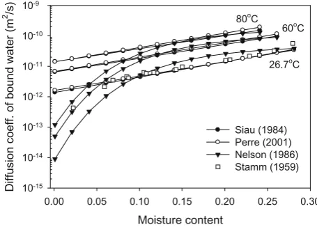
However, the coeffi cients given by Eqs. 19–21 are close to the experimental results found by Stamm18

at 26.7°C, and change little at higher temperatures, as shown in Fig. 2. They increase with increasing moisture content and temperature.

The activation energy is one of the kinetic energies that is necessary for the bound water to move from one sorption site to another, which is lower than the energy needed to evaporate bound water. However, its physical meaning seems to be unambiguous because it can be measured only by diffusion coeffi cient experiments and their gradient by temperature.

E R D

I RT D T b m m = − ⎡∂_{∂( )} ⎣⎢ ⎤ ⎦⎥ = ∂( ) ∂ ⎡ ⎣⎢ ⎤⎦⎥

(ln ) ln

1

2

(22)

Nelson20,21 investigated the activation energy of bound water theoretically. He stated that it consists of the energy needed to dissociate a mole of sorbed water from sorption sites (Ea) and the activation energy of liquid water (Ew). Ea

Moisture content

0.00 0.05 0.10 0.15 0.20 0.25 0.30

Diffusion coeff. of bound water (m

2 /s) 10-15 10-14 10-13 10-12 10-11 10-10 10-9 Siau (1984) Perre (2001) Nelson (1986) Stamm (1959) 26.7o C 60o C 80o C

Fig. 2. Bound water diffusion coeffi cient of cell wall in the transverse direction with moisture content and temperature

T

a

ble

3.

Heat and mass transfer coeffi

cients below fi

ber saturation point for each model

Model K11 (m 2 /s) K12 (m

2 /s K)

K21

(m

2 K/s)

K22 (m 2 /s) Stanish a Du D Pp bS ow ow v _vg 1 1 − () + − () φ ρ ς ρ Dv D PP bS ow ow v vg 1 1 − () + − () φ ρ η ρ 1 1 1 ρ φς C hD hD u PP p bb S vv vg − () + − () ⎛ ⎝⎜ ⎞ ⎠⎟ 1 1 1 ρ λφ η C hD hD v PP p eff b b S vv vg +− () + − () ⎛ ⎝⎜ ⎞ ⎠⎟ Perre b D u D bP ow v + ρ v D ow v ρ 1 _ρ ρ C hD h D u p bo w b P v v + () 1 ρ λ C hD v p eff v v + () Pang c Du K bR ow ow vv v 1 − () + φ ρ ς ρ ρ _μ Dv K bR ow ow vv v 1 − () + φ ρ η ρ ρ _μ Δ h u C K v p vv v ρ ρ _μ 1 ρ λ ρ _μ C hv K p eff v vv v + ⎛ ⎝⎜ ⎞ ⎠⎟ Δ A vramidis d 71 0 11 6 ×− () − () −

₍₎

a Stanish et al.

13

b Perre et al.

7

c Pang

10

d A

vramidis et al.

consists of Ev and RT/n. The former is the energy change from the sorbed state to the liquid state, and the latter is the energy change from the liquid state to the activated state.

E E RT

n E E

RT b= v+ + w= v+ +

0 7. 22175 (23)

According to Nelson,19,20

the transverse diffusion coeffi -cient of bound water can be expressed as:

D

m m

m m bT=

×

− ( + )

⎛

⎝⎜ ⎞⎠⎟⎛ ++

− 7 88 10 2 0 9 0 685 0 9

0 685 0 9 2 653 0 9 6

.

. . .

. .

. .

⎝⎝ ⎞⎠exp⎛⎝−RTE ⎞⎠ b

(24)

At 26.7°C, Fig. 2 shows that there is good agreement between Nelson’s model and Stamm’s experimental results, but there is a tendency to underestimate the diffusion coef-fi cient of bound water at lower moisture content levels and to overestimate at higher ones. At higher temperatures, there is rather good agreement between the three models in the range of m > 0.1, but Eq. 24 represents a lower value than the other two models when m < 0.1.

Equation 24 is somewhat different from Eqs. 19–21 because Ev changes exponentially as a function of moisture content. The concept of Nelson’s model is useful for esti-mating Eb by wood species because Ev may depend on the physicochemical properties of wood and a given specimen.

Combined bound water diffusion

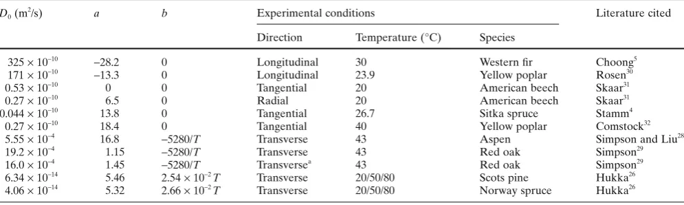
The conductivity of bound water depends on bound water diffusion through the cell walls and water vapor diffusion into the cell cavities. As discussed by Choong,5 the trans-verse moisture movement mechanism is dominated by cross-wall diffusion, which increases as moisture contents increase; whereas the longitudinal mechanism is dominated by vapor diffusion in the cell lumens, which decreases as moisture contents increase. This is supported by many experimental results, as shown in Fig. 3 and Table 4, and also by Danvind and Ekevad.22

The theoretical diffusion coeffi cient from the Avramidis model used in this study originates from Siau.2

It can be predicted more precisely for softwood, such as Scotch pine than for hardwood, such as aspen and red oak.

For convenience, the specifi c gravity of wood is assumed to be 0.40 for the calculation of heat and mass transfer coef-fi cients in this study. The combined or effective transverse diffusion coeffi cients of bound water (K11) for each model are shown in Fig. 4. The parameters necessary for the models are adopted in the literature as:

DbS

(

)

3 13

3 0 10. Stanish model

D m s m

T bP

2

9 9 9 8 4300

(

)

DbR

(

)

( )

− −

3 13 2 15

8 0 10. and 1 0 10.

Pang model

The transverse effective moisture diffusion coeffi cients in the Avramidis and Perre models are similar and increase

with increasing moisture content, because it is assumed that Perre included the porosity effect on DbP, and that the water vapor effect through the pit, Dv, is very small because af= 0.001. K11 in the Avramidis model is based on Siau,

2 which did not consider the effect of tortuosity and assumed that

a= 1.0.

However, the coeffi cients from Stanish’s and Pang’s models decrease with increasing moisture content because

DbS and DbR are constant, but z, u, and Dv decrease with increasing moisture content, which disagrees with most of the previous experimental results. All the models consid-ered in this study assume that all the phases are at the same temperature and that the partial vapor pressure is equal to its equilibrium pressure, whose condition is said to be in local thermodynamic equilibrium.

Stamm4

proposed an electrical model to simulate mois-ture transfer in the hygroscopic range (Fig. 5), shown in

Moisture content

0.00 0.05 0.10 0.15 0.20 0.25 0.30

Effective diffusion coefficent (m

2 /s)

10-11

10-10

10-9

10-8

10-7

Fig. 3. Comparison of transverse effective diffusion coeffi cients by theory and experiments during desorption at 60°C. Filled circles, Scots pine;26 _{fi lled triangles, Scots pine;}27 _{open triangles, Scots pine;}27 _{fi lled}

squares, aspen (transverse);28 _{open squares, red oak (transverse);}29 _{fi lled}

diamonds, theoretical (SG 0.30);2 _{open diamonds, theoretical (SG}

0.65)2

Moisture content

0.00 0.05 0.10 0.15 0.20 0.25 0.30

Moisture diffusion coefficinet (m

2 /s)

10-11

10-10

10-9

10-8

10-7

Avramidis(1992) Perre(1993) Stanish(1986) Pang(1997)

80oC

20oC

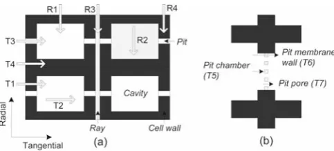
Fig. 6a. Figure 6b shows a simplifi ed model integrating sec-ondary paths through a pit. Because the resistance of T3 and T4 is large, Siau2

neglected their effects and adopted the model shown in Fig. 6d. As Siau stated, the effect of T3 may be important in woods with high permeability and high specifi c gravity, particularly at low moisture content and high temperature. The contribution of the pits in hardwood is expected to be less than in softwood because of the smaller pit openings in hardwoods.

However, Perre et al.7

considered T3 in their model and used the model from Fig. 6e, although Fig. 6f may be more suitable for woods according to Stamm’s theory. Stanish and Pang considered the movement of bound water and water vapor in the cavity by including the contribution of the pits as parallel paths. They adopted the model in Fig. 6g, and water vapor transfer through both the cavity and pit is more dominant than bound water. Therefore, their models are subject to some limitations for wood in the transverse direction and may be more suitable for moisture transfer through wood in the fi ber direction, wood-based panels (e.g., medium-density fi berboard and particleboard), and homogeneous porous material. For the models of Stanish and Pang, the dependence of combined diffusion coeffi cient on moisture content does not change even if the bound water and water vapor transfer is transformed to series dif-fusion such as Fig. 6d.

Thermal diffusion coeffi cient

Moisture is transported in the direction from higher tem-perature to lower temtem-perature, although there is no mois-ture gradient within a material, and is known as thermal diffusion or the Soret effect. Thermal diffusion is more important in building physics than drying because wood in service is rarely maintained in an isothermal state, and the nonisothermal state is relatively short during drying.

It should be noted that the Avramidis model originates from Siau,2 and Perre’s model did not consider the thermal diffusion effect. Stanish et al.13

compared their model to the experimental data from the literature.

The thermal diffusion coeffi cients (K12) of the three models are shown in Fig. 7, except for Pang’s model, whose value is several orders of magnitude lower than K11. These coeffi cients are found to increase with increasing moisture content and are observed to be higher in higher tempera-ture ranges. Pang’s model has a negative value in the entire hygroscopic range because −DbR(1 −f)h> vKvrv/mv, which

contradicts the phenomenological observation that mois-ture fl ows in the direction of decreasing temperamois-ture. The Stanish model also has a negative value at low moisture content due to the large entropy value of water vapor.

In the steady state, the Soret effect can be calculated by using dm/dT =−K12/K11 (Fig. 8). In the nonisothermal state, the moisture transfer rate decreases with increasing −dm/dT during drying, when the environmental temperature is higher than the material temperature.

The Avramidis model shows a higher value than Stan-ish’s model at 20°C, but it is close to the Stanish model at 80°C because there is little change with temperature in the Avramidis model. These two models show that the value increases with moisture content; however, it decreases with moisture content in the Perre model, and gives a constant value near zero over the whole moisture range. Therefore, Perre’s model cannot explain the Soret effect in steady state experiments.

Fig. 5. a Primary paths for tangential and radial moisture transport through a cell wall and b secondary paths through a pit5

Fig. 6a–g. The electrical analog models for the paths of tangential moisture transport

Moisture content

0.00 0.05 0.10 0.15 0.20 0.25 0.30

Thermal diffusio

n coefficient (m

2 /s K)

10-17

10-16

10-15

10-14

10-13

10-12

10-11

10-10

10-9

Avramidis Perre Stanish Pang 20oC

80oC

Figure 9 shows the results of comparison of the Avrami-dis, Stanish, and other models, and the relevant equations from the literature are shown in detail in Table 5.

Stanish9

compared his model to Models 2 and 7 in the unsteady state. As he stated, the accuracy of Model 7 must be questionable because it has a negative value over the whole moisture range. Peralta and Skaar23

compared the steady-state uniaxial moisture profi les to those predicted by fi ve different theoretical models. Models 9 and 5 provided the best results. Model 4 gave the next best prediction, fol-lowed by Model 6 (which is based on the Stanish model), and the last was Model 2. Siau and Avramidis24

compared three models (2, 8, and 9); Model 9 provided the best fi t to the experimental results, and Model 2 gave the poorest results.

There is little difference between Models 5 and 9 below moisture content of 0.2%, but they deviate greatly above that. Model 1 does not consider the material’s hygroscopic properties, so with hygroscopic material −dm/dT should be lower than that in Model 1. Avramidis and Hatzikiriakos25 compared Models 4 and 9 with drying experiments and concluded that the thermodiffusion coeffi cient of Model 9 resulted in the best fi t with the moisture and temperature

data. Therefore, it may be concluded from the above research that Model 9 is the best one to use for the noniso-thermal modeling.

Equation 23 and Model 5 show that the diffusion coeffi -cient of bound water decreases, and the Soret effect increases as the differential heat of sorption increases.

Heat diffusion and moisture thermodiffusion

The same values of volume heat capacity (rCp) and heat

transfer coeffi cient (leff) were adapted to all the models. As

shown in Table 3, however, the additional term of heat dif-fusion coeffi cient (K22) made the thermal conductivity vary between models because the condensation or sorption heat occurs in the direction of increasing temperature as the moisture content increases or decreases. As shown in Fig. 10, Perre’s and Pang’s models at all temperatures, and Stan-ish’s model at 20°C, show similar trends, with K22 decreasing at increasing moisture content, which was very close to the changes in leff/rCp. However, in Stanish’s model it remains

constant with moisture content at higher temperature (80°C), whereas in the Avramidis model there is a trend of

Moisture content

0.00 0.05 0.10 0.15 0.20 0.25 0.30

-dm/dT

(K

-1 )

-0.02 0.00 0.02 0.04 0.06 0.08

Avramidis Perre Stanish Pang

20oC 80oC

Fig. 8. Plot of −dm/dT against moisture content with oven-dried

spe-cifi c gravity of 0.4 at 20°C and 80°C

Moisture content

0.00 0.05 0.10 0.15 0.20 0.25

-dm/dT

(K

-1 )

0.00 0.02 0.04 0.06 0.08

Model 1 Model 2 Model 3 Model 4 Model 5 Model 6 Model 7 Model 8 Model 9

Fig. 9. Plot of −dm/dT against moisture content with oven-dried

spe-cifi c gravity of 0.4 at 50°C

Table 4. Comparison of parameters in effective diffusion equation Db= D0exp(aX + b) from experimental results in the literature

D0 (m

2_{/s) a b Experimental conditions Literature cited}

Direction Temperature (°C) Species

325 × 10−10 _{−28.2 0 Longitudinal 30 Western fi r Choong}5

171 × 10−10 _{−13.3 0 Longitudinal 23.9 Yellow poplar Rosen}30

0.53 × 10−10 _{0 0 Tangential 20 American beech Skaar}31

0.27 × 10−10 _{6.5 0 Radial 20 American beech Skaar}31

0.044 × 10−10 _{13.8 0 Tangential 26.7 Sitka spruce Stamm}4

0.27 × 10−10 _{18.4 0 Tangential 40 Yellow poplar Comstock}32

5.55 × 10−4 _{16.8 −5280/T Transverse 43 Aspen Simpson and Liu}28

19.2 × 10−4 _{1.15 −5280/T Transverse 43 Red oak Simpson}29

16.0 × 10−4 _{1.45 −5280/T Transverse}a _{43 Red oak Simpson}29

6.34 × 10−14 _{5.46 2.54 × 10}−2 _{T Transverse 20/50/80 Scots pine Hukka}26

increasing K22 at higher moisture contents. If K22 from Eq. 25 were adopted, the heat diffusion coeffi cient would exhibit a lower value than in the Avramidis model

K C

E C

C E

T K

RT m p

eff

b p

p b

22 11

1

0 018

= + ⎛_⎝ ⎞_⎠ ∂

∂ ⎛ ⎝⎜ ⎞⎠⎟ ⎛

⎝⎜

⎞ ⎠⎟

ρ λ

ρ ϕ

ϕ

. (25)

The Dufour effect, or moisture thermodiffusion, which causes the heat fl ux resulting from moisture diffusion, is shown in Fig. 11. However, there is little experimental evi-dence of the Dufour effect because it cannot be easily

mea-Table 5. Comparison of the ratio of moisture content gradient to temperature gradient (dm/dT) from the literature

Model Equation Literature cited

1

−v

u

Bramhall33

2

− − ∂

∂

( )

E RT

m E

m

b b

T 2

Skaar and Siau34

3

−ϕ

(

)

μ _ϕ

Td

dT E RT C

w

s ln

Siau35

4

−ϕ

(

)

μ _ϕ

Td

dT E E E RT C

w

b v s ln

Siau and Zin36

5 E E C T

T RT T

v+ s− pv

− −

( 1 038 0 049. . ) −( lnϕ)

Nelson20,21

6

− ϕTS

C

v Peralta and Skaar

23

7

−ϕ

(

)

μ _ϕ

Td

dT E E RT C

w

b s ln

Siau37

8

−ϕ

(

)

μ _ϕ

Td

dT E RT C

b

b ln

Siau and Avramidis24

9

− ϕE

C

b Siau and Avramidis,24 Peralta and Skaar23

C RT m T

= ∂

∂ ⎛ ⎝ ⎞⎠

2 ϕ

Moisture content

0.00 0.05 0.10 0.15 0.20 0.25 0.30

Heat diffusion coefficient (x10

7 , m 2 /s)

1.0 1.2 1.4 1.6 1.8 2.0 2.2 2.4

20oC

80oC

Fig. 10. Heat diffusion coeffi cient of wood with oven-dried specifi c gravity of 0.4 at 20°C and 80°C. Filled circles, Avramidis model; open circles, Perre model; fi lled triangles, Stanish model; open triangles, Pang model; crosses, Eq. 25

sured as the heat diffuses so much more rapidly through wood than does moisture. Therefore, it was diffi cult to determine what model was more appropriate for explaining moisture thermodiffusion. In addition, the effect of mois-ture thermodiffusion on the heat transfer rate may not be signifi cant because the heat diffusion is much faster than the moisture diffusion.

The moisture thermodiffusion coeffi cient (K21) from the Avramidis model increased with increasing moisture content, which is due to a function of the activation energy of bound water. For the other three models, it decreased with increasing moisture content because the enthalpy of bound water (hb) increases with moisture content.

Moisture content

0.00 0.05 0.10 0.15 0.20 0.25 0.30

Moisture thermo-diffusion coefficient (m

2 K/s)

10-11

10-10

10-9

10-8

10-7

10-6

10-5

10-4

Avramidis Perre Stanish Pang

20o

C 80oC

Conclusions

The driving potential for bound water may differ among researchers, and can be expressed in terms of a number of different state variables. Under isothermal conditions, it does not matter which potential is used in the diffusion equation as long as the appropriate diffusion coeffi cient is used.

Except for the Avramidis model, the other three models (Stanish, Perre, and Pang) were developed mainly for mod-eling high-temperature drying above the FSP. The transfor-mation of the four models with different state variables to the same forms results in different phenomenological trans-port coeffi cients by moisture content and temperature. There is a certain degree of confusion about the material parameters. This confusion arises from the use of different mathematical expressions and the driving forces assumed. In the case of the isothermal mass transfer coeffi cient, the moisture diffusion coeffi cient in the transverse direction by the Stanish and Pang models increased with deceasing moisture content. This contradicts the Avramidis and Perre models as well as numerous experimental results.

The effect of thermal diffusion on the drying process may not be predominant because the nonisothermal state is relatively short. Therefore, Perre’s model, which does not consider the thermal diffusion effect, has been used success-fully in the drying simulation. However, it may be errone-ous in certain cases when the nonisothermal state prevails over the system, such as building physics. The thermodiffu-sion coeffi cient, such as from Model 9, may be involved in Perre’s model.

Model 9 is more suitable than Model 4 for the Avramidis model. The water vapor movement through the pit should be involved in case of wood with high permeability and high specifi c gravity, particularly at low moisture content and high temperature, when calculating the moisture diffusion coeffi cient (Fig. 6b).

Therefore, the application of a model to various wood species would be questionable under a wide range of exter-nal conditions, although all four models were verifi ed by experimental results, and satisfactory agreements were obtained for a given material and set of environmental conditions. When developing and adopting new models, examination of whether the transport coeffi cients have physical meaning and are appropriate over the range of moisture content and temperature under consideration is required.

Acknowledgement This work was supported by the Korea Research Foundation Grants funded by the Korean Government (MOEHRD) (The Regional Research Universities Program/Biohousing Research Institute and KRF-2007-314-F00021).

References

1. Hameury S (2005) Moisture buffering capacity of heavy timber structures directly exposed to an indoor climate: a numerical study. Build Environ 40:1400–1412

2. Siau JF (1984) Transport processes in wood. Springer, Berlin Heidelberg New York, p 245

3. Avramidis S, Englezos P, Papathanasiou T (1992) Dynamic non-isothermal transport in hygroscopic porous media: moisture diffu-sion in wood. AIChE J 38:1279–1287

4. Stamm AJ (1960) Combined bound-water and water vapor diffu-sion into Sitka spruce. Forest Prod J 10:644–648

5. Choong ET (1963) Movement of moisture through a softwood in the hygroscopic range. Forest Prod J 13:489–498

6. Siau JF (1995) Wood: infl uence of moisture on physical properties. Virginia Polytechnic Institute and State University, Blacksburg, p 227

7. Perre P, Moser M, Martin M (1993) Advances in transport phe-nomena during convective drying with superheated steam and moist air. Int J Heat Mass Transfer 36:2725–2746

8. Whitaker S (1977) Simultaneous heat, mass, and momentum transfer in porous media: a theory of drying. Adv Heat Transfer 13:119–203

9. Stanish MA (1986) The roles of bound water chemical potential and gas phase diffusion in moisture transport through wood. Wood Sci Technol 19:53–70

10. Pang S (1997) Relationship between a diffusion model and a trans-port model for softwood drying. Wood Fiber Sci 29:58–67 11. Kamke FA, Vanek M (1994) Comparison of wood drying models.

Proceedings of 4th IUFRO International Wood Drying Confer-ence, Rotorua, New Zealand, pp 1–21

12. Yeo H, Smith WB (2005) Development of a convective mass trans-fer coeffi cient conversion method. Wood Fiber Sci 37:3–13 13. Stanish MA, Schajer GS, Kayihan F (1986) A mathematical model

of drying for hygroscopic porous media. AIChE J 32:1301–1311 14. Bories S (1988) Recent advances in modelisation of coupled heat

and mass transfer in capillary-porous bodies. Proceedings of 6th International Drying Symposium, pp 46–62

15. Akanni KA, Evans JW (1987) Effective transport coeffi cients in heterogeneous media. Chem Eng Sci 42:1945–1954

16. Forest Products Laboratory (1999) Wood handbook: Wood as and engineering materials. USDA Forest Service, Forest Products Lab., Madison

17. Simpson WT (1971) Equilibrium moisture content prediction of wood. Forest Prod J 21:48–49

18. Stamm AJ (1959) Bound-water diffusion into wood in the fi ber direction. Forest Prod J 9:27–32

19. Perre P, Turner IW (2001) Determination of the material property variations across the growth ring of softwood for use in a hetero-geneous drying model. Part 2. Use of homogenization to predict bound liquid diffusivity and thermal conductivity. Holzforschung 55:417–425

20. Nelson RM (1986) Diffusion of bound water in wood. Part 2: a model for isothermal diffusion. Wood Sci Technol 20:235–251 21. Nelson RM (1986) Diffusion of bound water in wood. Part 3: a

model for nonisothermal diffusion. Wood Sci Technol 20:309–328 22. Danvind J, Ekevad M (2006) Local water vapor diffusion coeffi

-cient when drying Norway spruce sapwood. J Wood Sci 52:195– 201

23. Peralta PN, Skaar C (1993) Experiments on steady state noniso-thermal moisture movement in wood. Wood Fiber Sci 25:124– 135

24. Siau JF, Avramidis S (1993) Application of a thermodynamic model to experiments on nonisothermal diffusion of moisture in wood. Wood Sci Technol 27:131–136

25. Avramidis S, Hatzikiriakos SG (1995) Convective heat and mass transfer in nonisothermal moisture desorption. Holzforschung 49:163–167

26. Hukka A (1999) The effective diffusion coeffi cient and mass trans-fer coeffi cient of Nordic softwoods as calculated from direct drying experiments. Holzforschung 53:534–540

27. Rosenklide A, Arfvidsson J (1997) Measurement and evaluation of moisture transport coeffi cients during drying of wood. Holz-forschung 51:372–380

28. Simpson WT, Liu JY (1991) Dependence of the water vapor dif-fusion coeffi cient of aspen (Populus spec.) on moisture content. Wood Sci Technol 26:9–21

30. Rosen HN (1976) Exponential dependency of the moisture diffu-sion coeffi cient on moisture content. Wood Sci 8:174–179 31. Skaar C (1958) Moisture movement in beech below the fi ber

satu-ration point. Forest Prod J 8:352–357

32. Comstock GL (1963) Moisture diffusion coeffi cients in wood as calculated from adsorption, desorption, and steady state data. Forest Prod J 13:97–103

33. Bramhall G (1979) Sorption diffusion in wood. Wood Sci 12:3–13 34. Skaar C, Siau JF (1981) Thermal diffusion of bound water in wood.

Wood Sci Technol 15:105–112

35. Siau JF (1983) Chemical potential as a driving force for noniso-thermal moisture movement in wood. Wood Sci Technol 17:101–105

36. Siau JF, Zin Z (1985) Nonisothermal moisture diffusion experi-ments analyzed by four alternative equations. Wood Sci Technol 19:151–157