Path Analysis Step by Step Using Excel
Akinnola N. AKINTUNDE*
Abstract
Quantifying the contribution of causal variables to a targeted effect variable directly and indirectly through other variables has always being the layer that researchers seldom examine. Path analysis method may be a natural extension to regression analysis where researchers may be able to quantitatively examine the direct contributions to the effect variable and the indirect effects through other vari-able to the effect varivari-able. Researchers are sometimes forced to stop their investigation at regression analysis level even when their model reports highly positive fit but could not find or explain any direct positive significant contribution from any of the causal variables in the system. It is a decision support tool that helps researchers determine the contribution of each variable to the effect and each variable via other variables to that effect. This paper gives us a step by step approach to doing path analysis using the Microsoft office Excel software. A tool most common to PC’s based on Microsoft windows operating systems and its users.
Keywords: Path analysis, path coefficient, causal factors, effect variables, multiple regressions, standardized variables, direct path coefficient, indirect path coefficient.
Introduction
The path coefficient method was pioneered by Prof.
Sewall Wright (1921, 1960). The work was only related to
population genetics at first. Now it is being applied in all
works of life.
Path Analysis extends multiple regression analysis, but while regression gives the best or closest prediction of the response variable based on the given causal factors by the method of least squares, path analysis goes further by pro-viding probable interpretation of the relationships between and within the contributing causal factors to the observed effects.
Y = a+b1X1 +b2X2 +b3X3 + U (eq .1)
The case of multiple regression in the equation above looks at a single response variable as a function of several causal / explanatory variables with the assumptions that values of variables are random, normally distributed and that the causal variables are independently contributing to the response variable.
p01 X1 + p02 X2 + p03 X3 + U = Y (eq. 2)
Path analysis (eq. 2) on the other hand, examines sev-eral explanatory variables as a function of the response
lating to contribute to the response variable. In other words causal factors are not acting independently.
Methodology
Any computer that will accommodate the windows
op-erating system that runs the Microsoft office Excel should
be adequate for the practical demonstration of the ways to do path analysis.
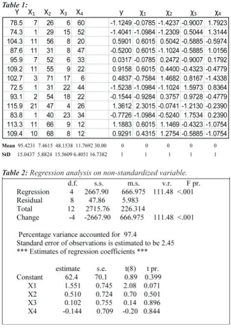
The data for our analysis is taken from (Li, 1975). This
data is standardized before a regression analysis is carried out using excel. Regression on a standardized variable/s gives partial regression coefficients unlike regression on non-standardized variables that gives concrete regression coefficients.
This contains one dependent variable Y and four inde-pendent variables X1…X4 (13 cases), applying the equa-tion x* = (x-m)/sd to the raw data on the left results in the
Table 2: Regression analysis on non-standardized variable.
Table 3: Regression analysis on standardized variable.
SUMMARY OUTPUT
Regression Statistics Multiple R 0.991148637
R Square 0.98237562
Adjusted R Square 0.973563431 Standard Error 0.162593508
Observations 13
ANOVA
df SS MS F Significance F
Regression 4 11.78854 2.947136 111.4792 4.76E-07
Residual 8 0.211493 0.026437
Total 12 12.00004
Coefficients Standard Error t Stat P-value Lower 95%Upper 95% Intercept -7.27325E-06 0.045095 -0.00016 0.999875 -0.104 0.103983
X1 0.606513438 0.291221 2.08266 0.070822 -0.06504 1.27807 X2 0.527707059 0.748672 0.704858 0.500901 -1.19873 2.254148 X3 0.043389586 0.32133 0.135031 0.895923 -0.6976 0.784378 X4 -0.160287849 0.788919 -0.20317 0.844071 -1.97954 1.658963
Direct Path Coefficient
Regression analysis on a set of standardized variables results in partial regression coefficients. Partial regression
coefficients are in fact another name for direct path coefficients.
and X4
The indirect contributions of X1 to Y will include X1 to
Y through X2, X3 and X4. The same applies to X2, X3 and X4 Standardizing variables in Ms Excel
Consider the example in the methodology section of
this paper. The initial values of the five variables are trans
-formed to generate the standardized version by first finding the mean and standard deviation of each unstandardized variable in Excel (I am assuming that my audience can do
this) and then for each variable, creating a corresponding
column to hold the standardized values of the variables by
applying this formula x* = (x-m)/sd. An example is to take each value x of big Y, subtracting the mean obtained for big Y and then divide the result by the standard deviation (sd) obtained for big Y. Do this repeatedly until all 13 cases of the big Y values are exhausted. Then you have a set of
standardized values for Y.
These values can then be placed in a corresponding
field for small y. Repeat the same procedure for all other
variables in the equation/dataset and the whole dataset is transformed. This procedure is simpler if you are familiar
with how to include Excel functions in your spread sheets columns. Excel will automatically calculate the values and
place it in the column you indicate for the result for each
variable →
(x* = (x-m)/sd)
In practice
The first step is to open your excel data file like in sample frame 1 below, highlight the first data column as in
the frame. Observe the last line giving the initial statistics (Average, Count and sum). These basic statistics will form the base for calculating the standard deviation and your
standardization process.
Repeat the same for all the variables in your excel file
and obtain the relevant basic statistics that will support
As an alternative, you can insert excel functions into whatever positions you desire to place your basic statistics like in sample frame 2. In this case I had placed the de-sired statistics below the columns of raw data. This is more relevant as I can then reference each of this cells relative position for my subsequent calculations. The example in
sample frame, highlights cell B17 where I want to place
the value calculated from my function placed at the point of the arrow above, it calculates the standard deviation of the values in cell b2 to b14.
The result of that calculation is placed in cell b17 (15.04372 for Y). The same was repeated for X1 (C17),
X2(D17), X3(E17), and X4(F17). All that is required is to
change the reference positions of the cells in the function
below the arrow to B, C, D, E, & F accordingly. The differ -ence between this and calculating for the mean is instead of
STDEV(B2:B14), you have AVERAGE(B2:B14) placed
as the function.
Now that you are introduced to the excel function, the
process of standardizing your raw values should become
easier. Now consider the (x* = (x-m)/sd) for
standardi-zation. Since you have the mean and standard deviation
for the variables in question, you can do your calculation
by brute force or do it using the Excel function STAND
-ARDIZE. It takes 3 arguments, the value of the variable to standardize, its mean and its standard deviation. As an example to standardize the first value of Y, you will insert into the function box =STANDARDIZE(B2,B16,B17), or better still =STANDARDIZE(B2,95.423,15.044) using the later in the first cell to be calculated will allow you to drag
the formula down for all cells under Y variable since the
mean and STDEV is common for all the values of Y to generate the series of standardized values.
Sample Frame 1 Sample Frame 2
Standardizing values for Y,
Having obtained your series of standardized values for the 5 variables Y, X1, X2, X3, & X4 you now have a
table that looks like the one on our methodology section. All that is required at this point is to carry out regression
analysis on the new standardized variables specifying Y as
variables.
The resultant coefficients for X1, X2, X3 and X4 are called partial regression Coefficients in other words, the
direct contribution of the X’s individually to the Dependent
variable Y. This is the Direct Path Coefficients of the causal
factors to the effect variable.
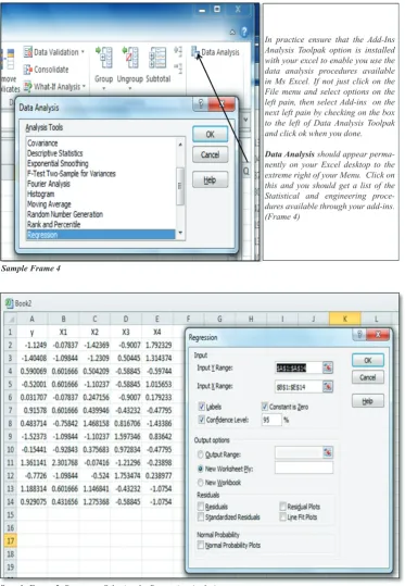
Sample Frame 4
Sample Frame 5: Parameter Selection for Regression Analysis
In practice ensure that the Add-Ins Analysis Toolpak option is installed with your excel to enable you use the data analysis procedures available in Ms Excel. If not just click on the File menu and select options on the left pain, then select Add-ins on the next left pain by checking on the box to the left of Data Analysis Toolpak and click ok when you done.
When you click on regression as the procedure you in-tend to use, you should get what looks like frame 5 above.
To the left are your standardized variables and to the right
is where you chose your regression parameters and the range of the cells for your Dependent (Y) and Independ-ent variables (X’s). Note that if you check labels as in the
box, it means that the first row of your data will be used as
labels. When you are done selecting your parameters and
defining your data range, click OK to get your output dis -played. An output similar to the one in methodology
sec-tion for standardized variables should be displayed.
Calculating Indirect Path Coefficients in Ms Excel
It is now a matter of multiplication and substitution
to calculate the indirect path coefficients and a number of ways can be employed. But going the Excel way will be
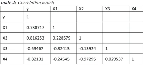
our focus. The only complement to our endeavour is to ob-tain the correlations matrix for the variables included in our equations and these I hope will be easy to our readers. Just in case it is not, I will explain how these are obtained
for our sample data through Excel.
Just refer back to the stage of choosing regression for
your analysis of the standardized variables, now instead of
regression choose Correlation and specify the parameters and the range for your data as you did for regression, do
not forget to check that the first row contains labels. When
you are done, click OK, a table like
Journal of Technical Science and Technologies the one below (Table 4) should be generated for you.
The next step towards obtaining our indirect path coeffi
-cients is to bring forth our direct path coeffi-cients gener -ated earlier (Table 5). With these two tables (Table 4 and Table 5), you can generate a table of indirect contributions for all variables in the equation.
Table 4: Correlation matrix.
From our regression analysis we obtained the table below
Table 5: Partial Regression Coefficients
Path analysis can be referred to as the process of
split-ting correlation coefficients into its component parts. It could be defined as the ratio of the standard deviation of
the effect due to a given cause to the total standard
devia-tion of the effect (direct path coefficient).
If Y is the effect and X1 is the cause, the path
coef-ficient for the path from cause X1 to the effect
As earlier mentioned under direct path coefficients cal -culation
the path coefficient from X1 to Y The indirect contributions of X1 to Y will include X1 through X2, X3 and X4. The same applies to X2, X3 and X4. The equation below illustrates the splitting process for a 3 factor causal variables with one effect variable Y
A sample run from a custom path analysis program
us-ing the previous sample data’s regression coefficients (1) If the correlation coefficient between a causal fac -tor and the effect is almost equal to its direct effect, then correlation explains the true relationship.
(2) If the correlation coefficient is positive, but the
direct effect is negative or negligible, the indirect effects seem to be the cause of correlation. In such cases, the
indi-(3) The correlation coefficient may be negative but the
direct effect is positive and high. In these circumstances, a way to selectively drop the undesirable indirect effects will have to be introduced. (Singh; Chaudhary, 1977)
(4) The residual effect determines how best the causal factors account for variability of the dependent variable. If the residual accounts for a large portion of the variability in the dependent variable, it then means that other causal variables have to be brought into the study as those being considered are not the causal factors directly responsible for the effect.
(5) A way to cross check / validate your result is to
add the direct path coefficient of a particular causal fac -tor to its indirect effects; the result should be equal to the
correlation coefficient between that causal factor and the
response variable. There may be some rounding errors and
these should be apparent. If your correlation coefficient is not equal to the total indirect + direct path coefficient, you
may want to double check on your data and your multiple
regression coefficients.
To achieve this on an excel template from our earlier practice should be easy, since all we have to do is set up two columns corresponding to
the Direct path coefficients and correlation matrix of respective cause
and effect variables and put in a function to multiply the values in the
two columns to generate the indirect coefficients.
A sample run from a custom path analysis program using the previous sample data’s
Conclusion
Successful prediction of consequences / effects de-pends on the recognition of the causes / factors contribut-ing to the system becontribut-ing predicted.
Many researchers stop shut at correlation coefficients
because the regression statistics they obtain from their data
looks unreal and they could not find alternative explana
-tion to the results. But knowing what to do and how to do it even with a simple tool like Ms. Excel when such oppor -tunity presents itself will enable researchers obtain further explanations on causes and effect variables and may there-fore encourage further research.
References
Afifi, A.A., Clark Virginia(1990): Computer-Aided Multi -variate Analysis Chapman & Hall, New York, USA ISBN 0-412-99021-0
Brown D., Rothery P. (1993): Models in Biology: Mathematics, Statistics and Computing, John Wiley & Sons Ltd, Chiches -ter, England ISBN: 0 471 93322 8
Gunst, R.F. & Mason, L. R. (1980): Regression Analysis and Its Application Marcel Dekker, Inc, New York, USA ISBN: 0-8247-69993-7
Li C.C. (1975): Path Analysis – a primer. The Boxwood press, Pacific Grove, California, USA ISBN: 0-910286-40-X Mansfield Edwin (1983): Statistics for business and economics,
2nd Ed., W.W. Norton & Company, Inc. New York, USA ISBN 0-393-95293-2
Microsoft Excel - Microsoft Corporations, One Microsoft Way Redmond, WA 98052-6399
Nie, H.N. & Hull, C.H., Jenkins J.G., Steinbrenner, K., Brent, D.H. (1975):Statistical Package for the Social Sciences – 2nd Edition McGraw-Hill, Inc, New York, USA ISBN 0-07-046531-2
SAS Institute Inc., (1990): SAS/STAT User’s Guide, Version 6, 4th Edition Vol. 1, Cary, NC, USA. ISBN 1-55544-376-1 Scheiner, M. & Gurevitch, J. (1993): Design and Analysis of
Ecological ExperimentsChapman & Hall, New York, USA ISBN 0-412-03561-8