Wing

MEASUREMENT DIFFERENCES RESULTING FROM

ANALYZING NATURAL RESOURCE SPATIAL DATABASES

REFERENCED TO MULTIPLE MAP COORDINATE SYSTEMS

Michael G. Wing

Forest Engineering, Resources, and Management, Oregon State University, Corvallis, OR, USA

Abstract.Map projection on-the-fly capability allows natural resource GIS analysts to geoprocess spatial

data layers referenced to different map coordinate systems. This study’s primary objective was to provide examples of spatial measurement differences that can result when point, line, and polygon natural resource spatial databases are referenced to different map coordinate systems and are used for a set of typical spatial analysis tasks. The GIS software used for evaluations was part of the ArcGIS product suite. We performed three separate spatial analyses: the intersection of spatial line features to polygons, the identity

of polygons with other polygons, and a spatial join analysis that involved several components. Four

separate spatial databases representing gauges, streams, watershed boundaries, and forest ownerships were each referenced to four different map coordinate system settings. An initial assessment of distances, areas, and categories of features resulting from geoprocessing tasks involved only spatial databases referenced to the same map coordinate system. The measurement and categorical results of this initial assessment became comparative benchmarks. Subsequent analyses involved the same geoprocessing tasks but mixed

databases referenced to different map coordinate systems. We found differences from the benchmark

values in many of the comparisons between databases of different map coordinate systems. There were relatively small measurement differences in the amount of line lengths measured within specific polygons resulting from overlay intersections between databases in different map coordinate systems. The identity of polygons with other polygons resulted in large area differences in some cases from initial baseline measurements, particularly when datums were substantially different (NAD 27 and WGS 84). Distance differences were greatest for the spatial joining of points to other point and line features when involving databases referenced to map coordinate systems with substantially different datums. Results indicate that GIS analysts using ArcGIS analysis tools should be cautious when analyzing spatial databases referenced to different map coordinate systems.

Keywords: GIS, map coordinate systems, map projections, geoprocessing

1

Introduction

Most geographic information systems (GIS) require that spatial data be referenced to a coordinate system in order to be viewed or used for analyses. A coordinate system references locations on the earth to a regularly spaced numeric set of measurements that facilitates lo-cation mapping. The coordinate system might be a rec-ognized map coordinate system (also referred to as a projected coordinate system as coordinates are some-times transformed in order to fit specific regions of the earth) that is associated with an actual location on the earth’s surface. The coordinate system might also be an assumed coordinate system (originating from an

ar-bitrary location) such as digitizing board coordinates or localized coordinates that are part of a specific measure-ment project. GIS have traditionally required that all databases in an analysis be referenced to the same coor-dinate system. More recently, some GIS allow for spatial databases that are referenced to different coordinate sys-tems to be simultaneously viewed or integrated into an analysis. This capability is sometimes referred to as on-the-fly map projection and requires that all databases, even if associated to a different location on the earth’s surface, are referenced to a recognized map coordinate system. The reference to a map coordinate system is typically accomplished through a projection file that is associated with the spatial database. On-the-fly map

Copyright c2011 Publisher of theMathematical and Computational Forestry & Natural-Resource Sciences

projection can facilitate mapping and analytical tasks among spatial databases referenced to different mapping coordinate systems by alleviating the need to ensure that all databases are referenced to the same coordinate sys-tem. When spatial databases require association with a different map coordinate system, GIS analysts typi-cally will use a “re-project” command and must choose from among a set of map coordinate parameters to cre-ate a new spatial database. The number of potential combinations of map coordinate parameters is vast and can sometimes create confusion for analysts due to the numerous choices (Wing and Bettinger 2008). Conse-quently, opportunities for error in this process abound, and as the result of a re-projection process, a second database must be integrated into subsequent work flow.

The on-the-fly projection process is not typically rec-ommended for analytical tasks since it produces an

ap-proximate match between spatial databases. A more

suitable application for on-the-fly map projections is to support visual examination of spatial databases or the creation of cartographic products where spatial databases need not always be perfectly registered to one another. ESRI’s ArcMap software is part of the ArcGIS suite that is among the world’s most popular GIS soft-ware. ArcMap supports on-the-fly map projection and does provide a warning to users when spatial databases have different map coordinate systems but allows ana-lytical processes between databases to continue in most cases. Many ArcMap users have likely ignored warn-ings and have proceeded with analytical tasks involv-ing spatial databases referenced to different map

coor-dinate systems. In addition, the risk of poor

analy-sis results by relying on map projections on-the-fly is sometimes not emphasized. The following text appears under the “Understanding Map Projections” section at the on-line ESRI ArcGIS 9.3 help document: “If your datasets have a well-defined coordinate system, then Ar-cGIS can automatically integrate your datasets with oth-ers by projecting your data on the fly into the appropri-ate framework—for mapping, 3D visualization, analysis, and so forth” (ESRI 2010).

The objectives of this study are to provide examples of the magnitude of spatial measurement differences that can result when point, line, and polygon (vector) natural resource databases are referenced to different map coor-dinate systems and are used in a set of typical spatial analysis tasks. Four separate spatial databases repre-senting gauges, streams, watershed boundaries, and for-est land ownerships were used in analyses tasks. The measurement difference examples provide an assessment of the potential risks that GIS analysts might encounter when relying upon on-the-fly projection for spatial anal-ysis tasks.

2

Methods

ArcMap 9.3 (ESRI 2004) and ArcToolbox 9.3 (ESRI 2008) GIS software was used for all spatial analyses. Four sets of point, line, and polygon vector databases

were created in an ESRI shapefile format. Vector

databases represent discrete objects (point, line, and polygon) and are perhaps the most common data struc-ture for GIS applications in forestry. The other primary data structure is raster and is better suited for contin-uous data such as elevation or imagery. The shapefile (*.shp) is one of the most popular formats worldwide for storing and exchanging vector spatial data. Each set contained the same group of point, line, and polygon vector features but each set was associated with one of four map coordinate settings. The first three map coor-dinate settings used three different datums for data lo-cated within Oregon, USA. A datum provides a frame or starting point that allows coordinates to be placed on a specific location on the earth’s surface (Wing 2008). The map coordinate systems included a specific state sys-tem known as the Oregon Lambert referenced to North American Datum (NAD) 1983, a state plane coordinate system in NAD 1927 (Oregon State Plane North), and a Universal Transverse Mercator (UTM) in World Geode-tic System (WGS 84), Zone 10 North. These coordi-nate systems are henceforth referred to as OLM 83, OSP 27, and UTM 84, respectively. The three different da-tums associated with these map coordinate systems were specifically chosen as they represent three of the most commonly applied datums for spatial databases. In ad-dition, the three primary coordinate systems each used a different coordinate unit: international feet, survey feet, and meters, respectively. These three coordinate units were chosen as they represent three of most commonly applied coordinate units for spatial databases. A fourth map coordinate system involved creating a set of vector databases that was referenced to the OLM 83 coordinate system but stripping each of the databases of the associ-ated projection file (*.prj). This left a coordinate system embedded in the databases but left the GIS software un-able to situate the databases on the earth’s surface. This coordinate system setting is referred to as OLM 83 strip.

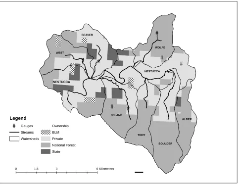
Each vector database set included a point file repre-senting weather gauges (referred to henceforth as gauge or gauges), a line file representing streams, and two poly-gon files representing watershed boundaries and forest land ownerships (Figure 1). The gauges database con-tained seven points and the streams concon-tained 87 lines. The watersheds database contained eight polygons each with a different watershed name. The forest land own-ership database had 24 polygons representing four dif-ferent forest land ownership categories.

#

_#

#

#

#

#

#

NESTUCCA

TONY WEST

NESTUCCA

FOLAND

WOLFE

BOULDER

ALDER BEAVER

Legend

#

Watersheds

Ownership

BLM

Private

National Forest

State

0 1.5 3 6Kilometers

–

Figure 1: Gauge, stream, watershed, and forest land ownership databases used in the map coordinate system analyses. Text on map figure represents watershed name.

a separate data frame within ArcMap. A data frame is a viewing perspective that allows a user to combine multiple databases into a single collection and to view any of the databases, either individually or in concert. ArcMap establishes a “home” map coordinate system for each data frame by examining the first spatial database that is added to a data frame. If the database contains a map projection file, the coordinate system described in the file is associated with the data frame. If the first spatial database doesn’t contain a map projection file, no coordinate system is associated, and the following warning appears, followed by the name of the database: “The following data sources you added are missing spatial reference information. This data can be drawn in ArcMap, but cannot be projected.”

If a database is referenced to a coordinate system and has a map projection file, and is added to a data frame

that contains databases that are referenced to a different coordinate system, a warning appears in a dialog box. The title of the dialog box is “Geographic Coordinate Systems Warning” and states that “Alignment and ac-curacy problems may arise unless there is a correct trans-formation between geographic coordinate systems.”

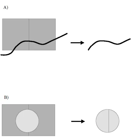
Vector lines were analyzed by intersecting each of the four stream databases with each of the four forest land ownership databases using ArcToolbox (Figure 2). We accepted all processing tool defaults during all

analy-ses. Each of the four different map coordinate

over-lap the polygon will be carried into the output database (Theobald 2007). A forest land ownership category is as-sociated with each intersected line, and a linear amount of stream is calculated for each ownership category. The linear measurements were recalculated for the output database, and the total length of streams in meters for each ownership category was used for comparisons.

Figure 2: Examples of A) an intersect command per-formed on a line with a rectangular polygon acting as the area of interest and B) an identity command per-formed on a rectangular polygon with a circular polygon acting as the area of interest.

Polygon areas were analyzed by using an identity com-mand on each of the four watershed databases with each of the four ownership databases using ArcToolbox (Fig-ure 2). Each of the four different map coordinate sys-tem versions of the watershed database was copied into the four different map coordinate system data frames within ArcMap. The identify command splits polygons at the geometric intersections with other polygons and outputs the results into a new polygon database. The re-sults will contain all portions of the initial database and any portions of a second database that overlap the ini-tial database (Wing and Bettinger 2008). A forest land ownership category is associated with each watershed as represented by the watershed name. The area measure-ments were recalculated for the output database, and the area of each ownership category was calculated for each watershed in square meters for analysis purposes.

Spatial joins were used to examine on-the-fly

projec-tion influences on point, line, and polygon vector files. A spatial join can be performed in ArcMap and exam-ines the proximity of feature locations in one database to feature locations in another database. A new output database is created as the result of a spatial join with the results dependent on whether points, lines, or polygons were involved. In this analysis, each of the four different map coordinate system versions of the gauge database was copied into the four different map coordinate sys-tem data frames. Each of the four gauge databases was then spatially joined to each of the four gauge, stream, and ownership databases. In the case of spatial joins to gauges and streams, the output database contains the distance to the nearest gauge and stream. The linear distance units are given in the same units as the map co-ordinate system of the initial database. These distances were converted to meters to facilitate analysis. In the case of spatial joins to forest land ownership polygons, the output database contains the associated ownership category for each gauge location. The output of this spatial join of a point to polygon database is similar to what one would expect through an intersect overlay process; the attributes of the polygon layer that each point intersects should be associated with the point in the resulting output. If points are not coincident with polygon features, the nearest polygon and the distance to the nearest polygon are returned.

3

Results and Discussion

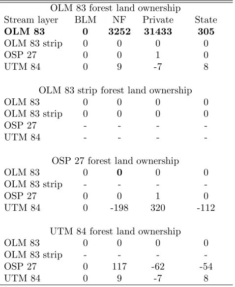
3.1 Lines Intersected with Polygons Stream vec-tor features referenced to each of the map coordinate set-tings were intersected with polygon features that were referenced to each of the map coordinate settings. The polygons contained an attribute that indicated one of four forest land ownership categories (Bureau of Land Management (BLM), National Forest (NF), Private, and State). Stream lengths were calculated from the layer that resulted from the intersect process. The intersec-tion of OLM 83 streams with OLM 83 forest land owner-ship polygons resulted in 3252 m for the NF ownerowner-ship, 31,433 m for the Private ownership, and 305 m for the State ownership (Table 1). The bold values in Table 1 contain the results of this initial comparison and are used as the baseline measurements for comparison. All other numeric values represent the difference from this base-line condition (a 0 indicates no difference), calculated by subtracting all other analysis results from the baseline. No streams were coincident with the BLM ownership locations in this analysis and resulted in no area being returned for this category.

Table 1: Stream lengths and distance differences (m)

resulting from intersection process.1

OLM 83 forest land ownership

Stream layer BLM NF Private State

OLM 83 0 3252 31433 305

OLM 83 strip 0 0 0 0

OSP 27 0 0 1 0

UTM 84 0 9 -7 8

OLM 83 strip forest land ownership

OLM 83 0 0 0 0

OLM 83 strip 0 0 0 0

OSP 27 - - -

-UTM 84 - - -

-OSP 27 forest land ownership

OLM 83 0 0 0 0

OLM 83 strip - - -

-OSP 27 0 0 1 0

UTM 84 0 -198 320 -112

UTM 84 forest land ownership

OLM 83 0 0 0 0

OLM 83 strip - - -

-OSP 27 0 117 -62 -54

UTM 84 0 9 -7 8

1_{Bold font indicates baseline measurements. All other}

mea-surement values are differences from baseline values.

OLM 83 strip streams with the ownership polygons for either OSP 27 or UTM 84. A warning appeared in the processing dialog box that indicated that empty

out-put would be generated. Examination of the output

database revealed no data and confirmed the warning message.

The results of the OSP 27 and UTM 84 stream inter-sections with the OLM 83 forest land ownership layer differed from those of the OLM 83 stream results. For OSP 27, the differences were only a meter for the Private category; all other lengths were identical to the OLM 83 results. For UTM 84, the differences were 9, 7, and 8 m for the NF, Private, and State ownerships, respectively. A slight difference was observed from the baseline dis-tances for the intersection of OSP 27 streams with OSP 27 forest land ownerships but this was only for the Pri-vate category for a one meter increment, identical to the intersection results of OSP 27 streams to OLM 83 ownerships. A similar trend was observed for the inter-section of UTM 84 streams to UTM 84 ownerships; the differences were modest (9, 7, and 8 m) but identical to those of the UTM 84 streams intersection with OLM 83 ownerships.

Measurement differences were most pronounced when OSP 27 streams were intersected with UTM 84 owner-ships, and when UTM 84 streams were intersected with OSP 27 ownerships. In the case of UTM 84 streams, measurement differences of 198, 320, and 112 m re-sulted from the OSP 27 intersection results. For OSP 27 streams, differences of 117, 62, and 54 m resulted.

3.2 Polygons Intersected with Polygons through an Identity Process

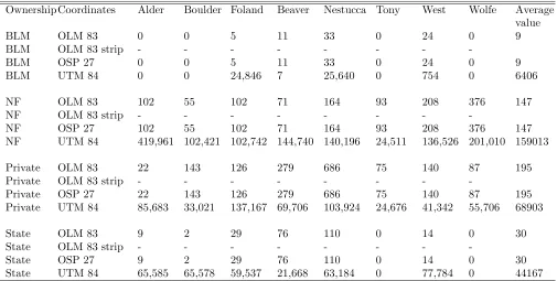
Vector polygons representing eight watershed areas classified by watershed name were intersected with the forest land ownership vector polygons for all map co-ordinate systems by using an identity process. Areas were calculated for each combination of watershed and ownership area as a means of comparison for the ini-tial results from the identity of OLM 83 watersheds and OLM 83 ownerships (Tables 2–5). Tables 2 to 5 list the results of the initial identity between these two layers in bold font. Other numeric values in the tables represent the difference between these baseline measurements and other identity results (a 0 indicates no difference), cal-culated by subtracting other identity area results from the baseline areas. An average value column gives the numeric mean of the measurements or differences.

For the initial identify between OLM 83 layers, areas

ranged from 57,549 to 15,839,263 m2_{. Results were}

iden-tical for watershed areas in each of the map coordinate systems when identitied with the OLM 83 ownership database. Four of the watersheds (Alder, Boulder, Tony, and Wolfe) did not have any coincident locations with the BLM ownership category. Two of the watersheds (Tony and Wolfe) did not have any coincident locations with the State ownership category.

Similarly to the streams and ownership intersection analysis results, the OLM 83 strip watershed databases could only be successfully identitied with forest land ownerships that were either in the OLM 83 or OLM 83 strip map coordinate systems. Area summaries for wa-tershed areas derived from successful identities of OLM 83 strip ownerships had no differences from the OLM 83 ownership results.

In comparison to the areas calculated by the identi-ties of the OLM 83 databases, there were relatively small differences in the area measurements that resulted from the identity of OSP 27 watersheds with OLM 83 own-erships. Although these differences were small, all OSP 27 results that were in coincident areas had differences. Differences of the OSP 27 watershed summaries for the

OLM 83 BLM and State ownerships were 110 m2 _or

less for identitied watersheds. The average differences for the OLM 83 NF and Private ownerships were 147

and 195 m2_{, respectively. The maximum difference was}

686 m2_{for the identity of the OSP 27 watershed named}

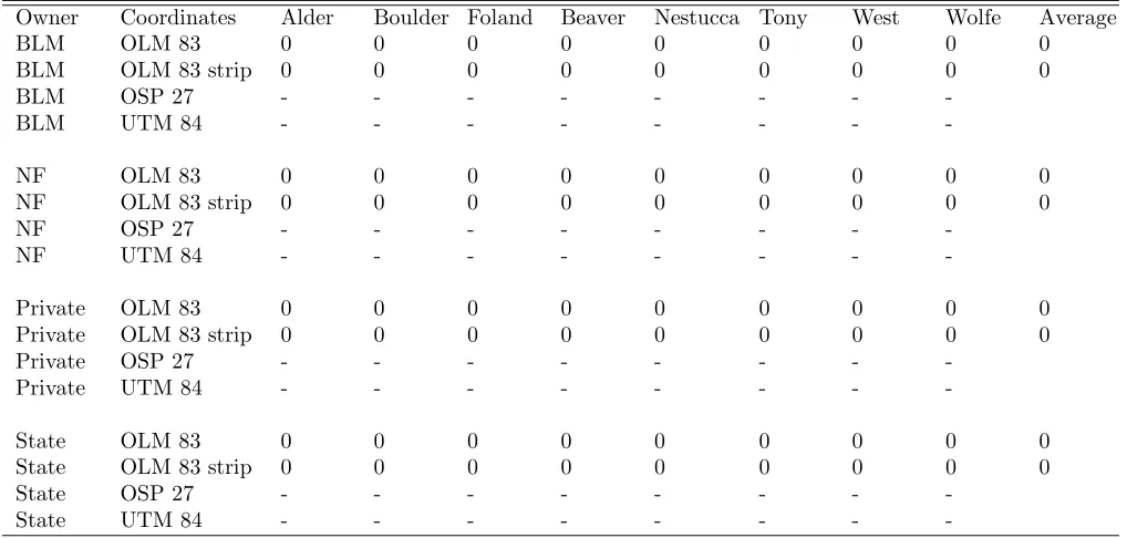
Table 3: OLM 83 strip watersheds: Area measurements (m2_{) resulting from identity of watershed and forest land}

ownership databases.1

Owner Coordinates Alder Boulder Foland Beaver Nestucca Tony West Wolfe Average

BLM OLM 83 0 0 0 0 0 0 0 0 0

BLM OLM 83 strip 0 0 0 0 0 0 0 0 0

BLM OSP 27 - - -

-BLM UTM 84 - - -

-NF OLM 83 0 0 0 0 0 0 0 0 0

NF OLM 83 strip 0 0 0 0 0 0 0 0 0

NF OSP 27 - - -

-NF UTM 84 - - -

-Private OLM 83 0 0 0 0 0 0 0 0 0

Private OLM 83 strip 0 0 0 0 0 0 0 0 0

Private OSP 27 - - -

-Private UTM 84 - - -

-State OLM 83 0 0 0 0 0 0 0 0 0

State OLM 83 strip 0 0 0 0 0 0 0 0 0

State OSP 27 - - -

-State UTM 84 - - -

-1_{Bold font indicates baseline measurements. All other measurement values are differences from baseline}

values or the average of the values in each row (average value column).

The differences for the OSP 27 watershed identity with the OSP 27 ownerships were relatively modest for the BLM and State ownerships with averages of 9 and

30 m2_{, respectively. The NF and Private ownership}

av-erage differences were slightly larger at 147 and 195 m2_,

respectively.

Differences were largest for the OSP 27 watershed and UTM 84 ownership identity processes. The differences were greatest for the NF ownership and ranged from

24,511 to over 419,961 m2 for the OSP 27 watershed

named Alder. Differences for the UTM 84 Private own-ership were also large and had a maximum of 103,924

m2for the OSP 27 watershed named Nestucca.

The UTM 84 watershed identities with ownership had the largest differences when OSP 27 databases were pro-cessed, especially with the NF and Private categories

which had average differences that exceeded 109,000 m2_.

Differences between the UTM 84 watersheds and the UTM 84 and OLM 83 ownerships were identical.

Aver-age differences were 2,464 m2 _{for the NF ownership; all}

other ownership categories had smaller differences.

3.3 Spatial Joins of Points to Point, Line, and Poly-gon Databases

A vector point layer of seven gauge locations was spa-tially joined to the point, line, and polygon databases using all combinations of the four map coordinate

rep-resentations. The point database was spatially joined to each gauge database, to each set of lines representing the streams, and to each polygon database representing the forest land ownership categories.

A map projection is usually required for all spatial databases that are part of a spatial join process in Ar-cMap. The OLM 83 strip databases could not be used in any of the spatial join processes with databases in other map coordinate systems. OLM 83 strip spatial joins were possible, however, with other databases that were associated with the OLM 83 strip map coordinate system.

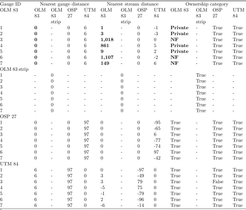
Distances for the OLM 83 gauges joined to the OLM 83 gauges were 0 m (Table 6). Table 6 lists the results of the initial join of OLM 83 gauges to other OLM 83 layers in bold. Other distances in the table represent the departure from this initial comparison. The OSP 27 gauge differences from the OLM 83 gauges were 0 m but the UTM 84 gauge distances were uniformly 6 m differ-ent from the baseline distance. Gauge distances were 0 m for the OLM 83 strip gauge spatial joins. The spatial joining of OSP 27 gauges to UTM 84 gauges resulted in differences of 97 m between gauges, regardless of which of these map coordinate systems was associated with the initial join layer.

Table 4: OSP 27 watersheds: Area measurements (m2_{) resulting from identity of watershed and forest land ownership}

databases.1

Ownership Coordinates Alder Boulder Foland Beaver Nestucca Tony West Wolfe Average

value

BLM OLM 83 0 0 5 11 33 0 24 0 9

BLM OLM 83 strip - - -

-BLM OSP 27 0 0 5 11 33 0 24 0 9

BLM UTM 84 0 0 24,846 7 25,640 0 754 0 6406

NF OLM 83 102 55 102 71 164 93 208 376 147

NF OLM 83 strip - - -

-NF OSP 27 102 55 102 71 164 93 208 376 147

NF UTM 84 419,961 102,421 102,742 144,740 140,196 24,511 136,526 201,010 159013

Private OLM 83 22 143 126 279 686 75 140 87 195

Private OLM 83 strip - - -

-Private OSP 27 22 143 126 279 686 75 140 87 195

Private UTM 84 85,683 33,021 137,167 69,706 103,924 24,676 41,342 55,706 68903

State OLM 83 9 2 29 76 110 0 14 0 30

State OLM 83 strip - - -

-State OSP 27 9 2 29 76 110 0 14 0 30

State UTM 84 65,585 65,578 59,537 21,668 63,184 0 77,784 0 44167

1_{Bold font indicates baseline measurements. All other measurement values are differences from baseline}

values or the average of the values in each row (average value column).

identified the nearest stream as being between 1 and 1107 m distant, depending on the gauge (Table 6). Streams referenced to the OSP 27 map coordinate sys-tem had no distance differences but UTM 84 stream dis-tance differences were between 0 and 6 m. OLM 83 strip gauge differences to OLM 83 strip streams were 0 m.

The spatial joining of OSP 27 gauges to OSP 27 streams and UTM 84 gauges to OSP 84 streams resulted in no differences (0 m). The spatial joining of OSP 27 gauges to UTM 84 streams resulted in differences, as did the joining of UTM 84 gauges to OSP 27 streams. Differences ranged between 6 and 97 m.

Outside of the problems in using OLM 83 strip databases in spatial join processes, the spatial joining of gauges to forest land ownership polygons had, with one exception, consistently correct associations of own-ership to gauge locations. Table 6 displays the owner-ship values using bold font that were returned by the initial spatial join of OLM 83 gauges to OLM 83 owner-ships. Values of True and False in the subsequent table indicate whether this initial association was matched by other comparisons. The one exception was gauge 3 of the UTM 84 map coordinate system that was falsely as-sociated with the Private ownership category of the OSP 27 map coordinate system, rather than the correct

cate-gory of NF. Closer inspection of this gauge revealed that it was within 50 meters of the border between these two categories, the difference in coordinate systems resulted in the incorrect association with the Private category.

4.0 Conclusion

The objectives of this study were to provide examples of measurement differences that can result when point, line, and polygon (vector) natural resource databases are referenced to different map coordinate systems and are used in a set of typical spatial analysis tasks. The GIS package examined was part of the suite of GIS software contained in ArcGIS.

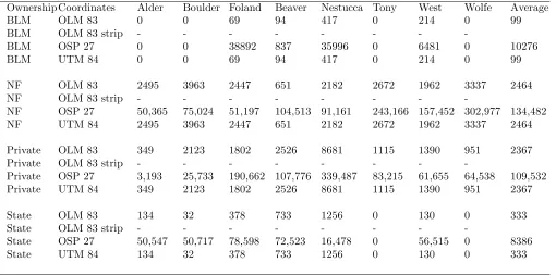
Table 5: UTM 84 watersheds: Area measurements (m2_{) resulting from identity of watershed and forest land ownership}

databases.1

Ownership Coordinates Alder Boulder Foland Beaver Nestucca Tony West Wolfe Average

BLM OLM 83 0 0 69 94 417 0 214 0 99

BLM OLM 83 strip - - -

-BLM OSP 27 0 0 38892 837 35996 0 6481 0 10276

BLM UTM 84 0 0 69 94 417 0 214 0 99

NF OLM 83 2495 3963 2447 651 2182 2672 1962 3337 2464

NF OLM 83 strip - - -

-NF OSP 27 50,365 75,024 51,197 104,513 91,161 243,166 157,452 302,977 134,482

NF UTM 84 2495 3963 2447 651 2182 2672 1962 3337 2464

Private OLM 83 349 2123 1802 2526 8681 1115 1390 951 2367

Private OLM 83 strip - - -

-Private OSP 27 3,193 25,733 190,662 107,776 339,487 83,215 61,655 64,538 109,532

Private UTM 84 349 2123 1802 2526 8681 1115 1390 951 2367

State OLM 83 134 32 378 733 1256 0 130 0 333

State OLM 83 strip - - -

-State OSP 27 50,547 50,717 78,598 72,523 16,478 0 56,515 0 8386

State UTM 84 134 32 378 733 1256 0 130 0 333

1_{Bold font indicates baseline measurements. All other measurement values are differences from baseline}

values or the average of the values in each row (average value column).

had a defined map projection. The measurement and categorical results of this initial assessment were used as benchmarks against which other analysis results could be made. Subsequent analyses involved analyzing layers that were registered to different map coordinate systems. We found differences from the benchmark values in many of the comparisons that were made between layers of dif-ferent map coordinate systems. These differences were relatively small in some cases, but were large in other instances.

These results indicate that GIS analysts working with ArcGIS analysis tools must take care when working with natural resource spatial databases that are referenced

to different map coordinate systems. There were no

measurement differences that occurred when layers refer-enced to the OLM 83 map coordinate system were com-pared to other layers that were in the same coordinate system yet lacked an associated map projection file (as in the case of OLM 83 strip layers in this study). It was not possible, however, to conduct a spatial join between such layers. It was possible to spatially join two layers that were referenced to the same map coordinate system but did not have map projection files; otherwise a map projection is required of both layers. Another limitation of not have an assigned map projection file witnessed in

this study was the inability to conduct overlay analyses (intersect and identify) with layers set to a different map coordinate system.

There were relatively small measurement differences in the amount of stream length that was measured within forest land ownership categories as the result of an intersect process between layers in different map co-ordinate systems. These differences appeared to be in-fluenced by the length of the streams for the UTM 84 to OSP 27 to comparisons: differences increased as stream lengths also increased. However, when the comparison was reversed (OSP 27 to UTM 84), the relationship was no longer consistent. Small differences from the baseline lengths were also observed between layers registered to the same map coordinate system; this is the result of the transformation that occurs within the geometry of line and polygon features as they are re-projected.

The identity of polygons with other polygons resulted in relatively large area differences from the initial

base-line measurements. The largest differences were

de-tected when comparing layers that were mixed between the OSP 27 and UTM 84 map coordinate systems. The comparison of OSP 27 watersheds to UTM 84 owner-ships resulted in area differences that did not appear to

compari-Table 6: Distances (m) and forest land ownership categories resulting from spatial joins of point, line, and polygon

databases.1

Gauge ID Nearest gauge distance Nearest stream distance Ownership category

OLM 83 OLM

83

OLM 83

OSP 27

UTM 84

OLM 83

OLM 83

OSP 27

UTM 84

OLM 83 OLM

83

OSP 27

UTM 84

strip strip strip

1 0 - 0 6 1 - 0 -1 Private - True True

2 0 - 0 6 3 - 0 -3 Private - True True

3 0 - 0 6 1,018 - 0 0 NF - True True

4 0 - 0 6 861 - 0 5 Private - True True

5 0 - 0 6 9 - 0 2 Private - True True

6 0 - 0 6 1,107 - 0 -2 NF - True True

7 0 - 0 6 149 - 0 6 NF - True True

OLM 83 strip

1 - 0 - - - 0 - - - True -

-2 - 0 - - - 0 - - - True -

-3 - 0 - - - 0 - - - True -

-4 - 0 - - - 0 - - - True -

-5 - 0 - - - 0 - - - True -

-6 - 0 - - - 0 - - - True -

-7 - 0 - - - 0 - - - True -

-OSP 27

1 0 - 0 97 0 - 0 -95 True - True True

2 0 - 0 97 0 - 0 -65 True - True True

3 0 - 0 97 0 - 0 6 True - True True

4 0 - 0 97 0 - 0 -77 True - True True

5 0 - 0 97 0 - 0 -74 True - True True

6 0 - 0 97 0 - 0 97 True - True True

7 0 - 0 97 0 - 0 -42 True - True True

UTM 84

1 6 - 97 0 0 - -97 0 True - True True

2 6 - 97 0 3 - -49 0 True - True True

3 6 - 97 0 3 - 79 0 True - False True

4 6 - 97 0 -5 - 75 0 True - True True

5 6 - 97 0 -1 - -79 0 True - True True

6 6 - 97 0 2 - -96 0 True - True True

7 6 - 97 0 -6 - -14 0 True - True True

1

Bold font indicates baseline measurements or ownership category. All other measurement values are differ-ences from baseline values.

True or false indicates whether the correct forest land ownership category was returned.

son of UTM 84 watersheds to NAD 27 ownerships, how-ever, resulted in differences that were slightly larger on average (when accounting for negative area results) and

moderately correlated with watershed area (r2 =0.55).

More modest area differences were also observed when comparing layers mixed between the OLM 83 and UTM 84 map coordinate systems. The smaller differences in the OLM 83 and UTM 84 comparisons is likely influ-enced by the more similar nature of the NAD 83 and WGS 84 datums that support these map projections.

The NAD 27 datum precedes both the NAD 83 and WGS 84 datums by over 50 years as it contains field measurements that were collected up through 1927. The NAD 83 and WGS 84 datums include measurements that were collected through 1983 and 1984, respectively, and are more similar to each other than to NAD 27.

involving layers that were registered to a mix of OSP 27 and UTM 84 map coordinate systems. The spatial join-ing of gauges to polygon features, akin to an intersect overlay process when layers are spatially coincident, had only one result that differed from the baseline. This dif-ference resulted from joining layers registered to the OSP 27 and UTM 84 map coordinate systems. Detected dif-ferences, overall, however were relatively modest in that they were less than 100 m. These modest differences are probably influenced by the short distances that typically separated features that were being spatially joined. The maximum distance that separated gauges from streams was 1107 m.

The shapefile format was used for spatial database

representation in this analysis. ESRI is now

encour-aging ArcGIS users to use the geodatabase format for spatial databases. To determine whether database for-mat might influence results, the UTM 84 watershed and OSP 27 ownership layers were converted into personal geodatabases and identitied. This comparison was se-lected as it had resulted in large area errors during the shapefile based analysis. The geodatabase results

dif-fered by an average of less than 3 m2 (maximum = 11

m2) from those produced by the shapefile comparisons,

an insignificant amount considering that each watershed and ownership combination covered an area in excess of

57,000 m2 (Tables 2–5). These findings suggest that

while data format does influence spatial data analysis between databases in different map projections, the ac-tual difference is negligible but analytical results still lead to potentially large measurement errors.

The likely reason for the differences in analytical re-sults between spatial databases registered to different map coordinate systems observed in this study is that the map projection on the fly process is unable to pro-duce a transformation solution that is as robust as that produced by a re-projection. A re-projection results in a new database being created that is associated with a different map coordinate system. In this process, the di-mensions of input point, line, and polygon objects are re-configured so that they conform to the earth’s surface as represented by the new output map coordinate system. A map projection that is applied on the fly can is a tem-porary process and one that likely results in a less

rigor-ous solution for coordinate transformations. Given that the on the fly projections may need to be re-calculated as a user shifts viewing perspective, such as that produced by zooming or panning tools, it may also be that on the fly projections result in differences that are subject to change. In addition, the influence of feature size (length of lines, area of polygons) may have an influence on an-alytical results drawn from spatial databases registered to opposing map coordinate systems. These uncertain-ties, and a broader treatment of the influence of spatial database formats on map projection differences, are sug-gested for future research.

Acknowledgements

The author gratefully acknowledges the assistance of Bryan L. Huck, Kyler Kokenge, Sam B. Lovelace, and Henk Stander with GIS measurements. In addition, the author thanks two anonymous reviewers for constructive comments.

References

Environmental Systems Research Institute (ESRI).

2004. ArcGIS 9: Geoprocessing in ArcGIS. ESRI

Press: Redlands, CA. 363 p.

Environmental Systems Research Institute (ESRI). 2008. ArcGIS 9: Using ArcMap. ESRI Press: Red-lands, CA. 585 p.

Environmental Systems Research Institute (ESRI). 2010. An overview of map projections. Available at: http://webhelp.esri.com/arcgisdesktop/9.3/index .cfm?TopicName=An overview of map projections [accessed 16 September, 2010].

Theobald, D.M. 2007. GIS concepts and ArcGIS meth-ods. Third Edition. Conservation Planning Technolo-gies, Fort Collins, CO. 440 p.

Wing, M.G. 2008. Keeping pace with GPS technology in the forest. Journal of Forestry 106(6):332-338.