Abstract— This paper provides a comparative evaluation of different supervised and unsupervised classification algorithm. A multivariate data set (iris dataset) is considered for the example and different supervised classification techniques such as Naive-Bayes classification, support vector machine (SVM) and different unsupervised classification techniques such as K-means, C-means, Fuzzy C-Means, Self-Organizing Map (SOM) are used for classification of the problem. A comparative evaluation is carried out between different algorithms.
Index Terms— iris dataset; Fuzzy C-means; K-means; support vector machine; Self-Organizing Map (SOM)
1) INTRODUCTION
One of the challenges of the large amounts of information stored in databases is to find or extract potentially useful, understandable and novel patterns in data which can lead to new insights. This is the goal of a process called Knowledge Discovery in Databases (KDD). The KDD process consists of several phases: in the Data Mining phase the actual discovery of new knowledge takes place.
Traditionally, parametric statistical approaches such as a discriminant analysis have been extensively used to classify one group from others based on the associated individual characteristics (or features). The main assumption required for the discriminant analysis is that these features follow a multivariate normal distribution with distinct means for each group and a common variance-covariance matrix. When this common variance-covariance matrix assumption is met for k groups, Fisher's linear discriminant function (DISC) is used for classification. When this assumption is violated, instead of a linear discriminant function, a quadratic discriminant function (QDISC) is estimated based on an individually estimated variance-covariance matrix. Due to a certain distributional assumption required for the features of discriminant analysis, many authors have used a logistic discriminant function (LOGID) or a nonparametric classification method such as K-nearest neighborhood (KNN). In logistic regression, the maximum likelihood estimation is used to find the probability of classifying a test item to one group as a function of associated individual features, where this probability is considered as a parameter
Manuscript received August, 2017
Ranjita Rout, Mukesh Bathre Department of Computer Science and
Engineering, Government College of Engineering, Kendujhar, Odisha, India ([email protected], [email protected])
of Bernoulli or multinomial distribution depending on the number of classes. Nonparametric methods do not make any distributional assumptions and classify a test case based on the training samples in the neighborhood of the item in terms of associated individual features. One of the most popular nonparametric methods is voting K nearest neighbor method. The KNN method classifies a test case into the class that supplies the largest number of neighbors among the K-nearest neighbors of the case.
This paper provides a comparative evaluation of different supervised and unsupervised classification algorithms for a multivariate data set.
This paper is organized as follows. Section II provides details about supervised classification techniques such as Naïve-bayes and support vector machine. Section III provides details about unsupervised classification techniques such as SOM, K-means, C-means, Fuzzy C means etc. Section IV provides simulation results. Section V concludes the paper.
2) SUPERVISED CLASSIFICATION TECHNIQUES Learning or adaptation is supervised when there is a desired response that can be used by the system to guide the learning. Decision trees and neural nets are two common types of supervised learning. This type of learning always requires a target variable to predict. Supervised learning algorithms have been used in many applications. Supervised learning involves the gathering of data to be used for data mining, identifying the target variable, breaking up of the data into training and testing data and developing the classifier. The training data is used by the data mining algorithm to „learn‟ the data and build a classifier. The test data is used to evaluate the performance of the classifier on new data. The performance a classifier is commonly measured by the percentage of incorrectly classified instances on the data used. Train error rate refers to the percentage of incorrectly classified instances on the training data and test error rate refers to percentage of incorrectly classified instances on the test data.
3) Naïve-bayes Classification
Naive Bayes algorithm is the algorithm that learns the probability of an object with certain features belonging to a particular group/class. The Naive Bayes algorithm is called "naive" because it makes the assumption that the occurrence of a certain feature is independent of the
Classification of Multivariate Data Set using
Supervised and Unsupervised Classification
Methods
occurrence of other features. Naïve-Bayes classification can be represented as
|
|
P A B P A
P A B
P B
An advantage of Naïve Bayes algorithm over some other algorithms is that it requires only one pass through the training set to generate a classification model. Naïve Bayes works very well when tested on many real world data sets [58]. Naïve Bayes can obtain results that are much better than other sophisticated algorithms. However, if a particular attribute value does not occur in the training set in conjunction with every class value, then Naïve Bayes may not perform very well. It can also perform poorly on some data sets because attributes were treated as though they are independent, whereas in reality they are correlated.
4) Support Vector Machine
Recently, support vector machines have been introduced for solving pattern recognition problems. In this method one maps the data into a higher dimensional input space and one constructs an optimal separating hyperplane in this space. This basically involves solving a quadratic programming problem, while gradient based training methods for neural network architectures on the other hand suffer from the existence of many local minima. Kernel functions and parameters are chosen such that a bound on the VC dimension is minimized. Later, the support vector method was extended for solving function estimation problems [3].
Fig. 1. Hyperplane of SVM
Let training set
1...
,
i i i n
x y
,x
i
R
d ,y
i
1,1
be separated by a hyperplane with margin ρ. Then for each training example
x y
i,
i
1
2
1
2
T i i T iw x
b
y
w x
b
y
For every support vector
x
s the above inequality is an equality. After rescaling w and b by ρ/2 in the equality, weobtain that distance between each
x
s and the hyperplane isT
w x b
r
w
Then the margin can be expressed through (rescaled) w and b
as
2r
2
w
5) UNITS
Unsupervised learning deals with finding clusters of records that are similar in some way. As discussed earlier, unsupervised learning does not require a target variable for analysis. Unsupervised learning is often useful when there are many competing patterns in the data, making it hard to spot any single pattern. Building clusters of similar records reduces the complexity within clusters so that other data mining techniques are more likely to succeed. In unsupervised learning, the main concern is in obtaining clusters in data that have useful patterns.
6) Self Organizing Map
The aim is to learn a feature map from the spatially continuous input space, in which our input vectors live, to the low dimensional spatially discrete output space, which is formed by arranging the computational neurons into a grid [1,2]. The stages of the SOM algorithm that achieves this can be summarized as follows:
Initialization: Choose random values for the initial weight
vectors
w
j.Sampling: Draw a sample training input vector
x
from the input space.Matching: Find the winning neuron
I x
that has weight vector closest to the input vector, i.e. the minimum value of
2 1 D j i ji id
x
x
w
Updating: Apply weight updation equation
,
ji j I x i jiw
t T
t
x
w
, j I xT
t
is a Gaussian neighbourhood,
t
is the learning rateContinuation: keep returning to step 2 until the feature map
stops changing.
7) Dendrogram
Dendrogram (tree) generates a dendrogram plot of the hierarchical binary cluster tree. A dendrogram consists of many U-shaped lines that connect data points in a hierarchical tree. The height of each U represents the distance between the two data points being connected. If there are 30 or fewer data points in the original data set, then each leaf in the dendrogram corresponds to one data point. If there are more than 30 data points, then dendrogram collapses lower branches so that there are 30 leaf nodes. As a result, some leaves in the plot correspond to more than one data point.
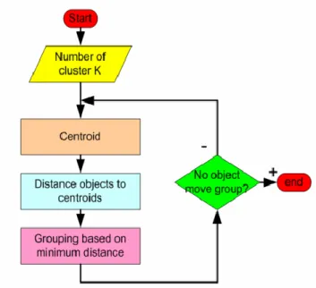
8) K-Means algorithm
The way k-means clustering works is that first the number of clusters (k) desired is specified, then the algorithm selects k cluster seeds (centers) which are located approximately uniformly in a multi-dimensional space. Each observation is then assigned to the nearest cluster mean to form temporary clusters. The cluster mean positions are then calculated and used as new cluster centers. The observations are then reallocated clusters according to the new cluster centers. This is repeated until no further change in the cluster centers occurs.
Given the cluster number K, the K-means algorithm is carried out in three steps after initialization:
Initialization: set seed points (randomly)
1) Assign each object to the cluster of the nearest seed point measured with a specific distance metric
2) Compute new seed points as the centroids of the clusters of the current partition (the centroid is the centre, i.e., mean point, of the cluster)
3) Go back to Step 1, stop when no more new assignment (i.e., membership in each cluster no longer changes)
Fig. 2. Flow chart of K-means clustering algorithm
9) Fuzzy C-means algorithm
Fuzzy c-means (FCM) is a data clustering technique in which a dataset is grouped into n clusters with every datapoint in the dataset belonging to every cluster to a certain degree. For example, a certain datapoint that lies close to the center of a cluster will have a high degree of belonging or membership to that cluster and another datapoint that lies far away from the center of a cluster will have a low degree of belonging or membership to that cluster. Fuzzy C-means algorithm is based on the minimization of objective function
2 1 1 N C m m ij i j i j
J
u
x
c
Fig. 3. Flow chart of fuzzy C-means algorithm
10) SIMULATION RESULTS
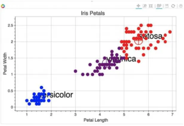
To analyze the performance of different supervised and unsupervised classification techniques, a very well-known multivariate dataset (Iris dataset) is considered [4,5]. In iris dataset, there are 4 attributes, 150 instances and no missing value. The dataset was created by R.A. Fisher and donated on July 1, 1988. The attributes of the dataset are (a) sepal length (cm), (b) sepal width (cm), (c) petal length (cm) and (d) petal width (cm). The three classes are (a) iris setosa, (b) iris versicolour and (c) iris virginica
Table I: Description of dataset
Attributes Min Max Mean SD Class Correlation Sepal length 4.3 7.9 5.84 0.83 0.7826 Sepal width 2 4.4 3.05 0.43 -0.4194 Petal length 1 6.9 3.76 1.76 0.949 Petal width 0.1 2.5 1.2 0.76 0.9565 *SD means standard deviation
Figure 4 shows the classification results of naïve-bayes classification algorithm.
Fig. 4. Classification results of Naïve-Bayes clasifier
Fig. 5. Architecture of Self-Organizing Map
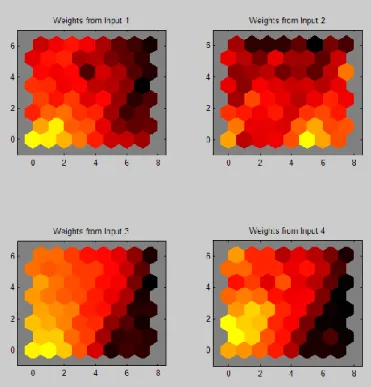
Figure 5 shows the architecture of Self-Organizing Map and Figure 6 shows the classification results of SOM classification algorithm. Figure 7 shows the classification results of dendrogram. Figure 8 shows the classification results of K-means classification algorithm. Figure 9 shows the classification results of fuzzy C-means classification algorithm. Figure 10 shows the classification results of C-means classification algorithm.
Fig. 6. Classification results of Self-Organizing Map
0 5 10 15 20 25 30
Fig. 7. Classification results of dendrogram
0 2 4 0 5 10 2 4 6 4 6 8 0 2 4 0 5 10 2 4 6 4 6 8
Fig. 8. Classification results of K-means algorithm
40 60 80 20 30 40 50 sepal length s e p a l w id th 1 2 3 1 2 3 40 60 80 0 20 40 60 80 sepal length p e ta l le n g th 1 2 3 1 2 3 40 60 80 0 10 20 30 sepal length p e ta l w id th 1 2 3 1 2 3 20 40 60 0 20 40 60 80 sepal width p e ta l le n g th 1 2 3 1 2 3 20 40 60 0 10 20 30 sepal width p e ta l w id th 12 3 1 2 3 0 50 100 0 10 20 30 petal length p e ta l w id th 1 23 1 2 3
Fig. 9. Classification results of fuzzy C-means algorithm
3 3.5 4 4.5 5 5.5 6 6.5 7 1 1.5 2 2.5 versicolor (training) versicolor (classified) virginica (training) virginica (classified) Support Vectors
Fig. 10. Classification results of C-means algorithm
11) CONCLUSION
This paper provides a comparative evaluation of different supervised and unsupervised classification algorithms. A test problem (iris dataset) is considered for classification and different classification techniques are used and performance
REFERENCES
[1] Pavel Stefanovic, Olga Kurasova, “Visual analysis of self-organizing maps,” Nonlinear Analysis: Modeling and Control, vol. 16, no. 4, 2011, pp. 488-504.
[2] S. Hasan, S.M. Shamsuddin, “Multistrategy self-organizing map learning for classification problems,” Computational Intelligence and Neuroscience, 2011, pp. 1-11.
[3] J.A.K Suykens, J Vandewalle, “Least square support vector machine classifiers,” Neural Processing Letters, 9, 1999, pp. 293-300. [4] R.A. Fisher, “The use of multiple measurements in taxonomic
problems,” Annual Eugenics, 7, part II, 1936, pp. 179-188. [5] UCI Machine learning repository, (web link)
[6] Subhransu Padhee, Nitin Gupta, Gagandeep Kaur, “Data driven multivariate technique for fault detection of waste water treatment plant,” International Journal of Engineering and Advanced Technology, vol. 1, issue 4, Apr. 2012, pp. 45-50.