Research Group
Design and implementation of a
database client application for
inserting, modifying, presentation and
export of bitemporal personal data
Diploma Thesis
Tobias Schlaginhaufen
Z¨urich, Switzerland
Student ID: 99-905-721
Professor: Prof. Klaus R. Dittrich
Supervisor: Boris Glavic
Date of Submission: April 30, 2007
University of Zurich
Department of Informatics (IFI)
There exists only little support for temporal data in conventional relational databases, although many applications require temporal or even bitemporal storage of data. This thesis describes the implementation of a bitemporal database and a pursuant client application, for managing study subjects of a longitudinal etiological study of adjustment and mental health.
Designing a bitemporal database on top of a relational database model in-volves the dilemma of using the well-established storage organization and query evaluation techniques of relational databases and accept a certain redundant storage of data or time-normalizing the data model and avoid redundancy but incur a degenarated relational model, which is complex, difficult to handle and may degrad the performance of a relation database system. We present an approach striking the balance between these two extremes.
Temporale Daten werden von konventionellen relationalen
Datenbanksyste-men noch kaum unterst¨utzt, obwohl viele Anwendungen die temporale oder
bi-temporale Speicherung von Daten ben¨otigen. Im Rahmen dieser Diplomarbeit
wird eine bitemporale Datenbank und eine dazugeh¨orige Client-Anwendung
erstellt, um Probanden einer ¨atiologische Langzeitstudie zur psychischen
Ge-sundheit zu verwalten.
Das Entwicklung einer bitemporalen Datenbank auf einem relationalen Da-tenmodell bringt das Dilemma mit sich, entweder die etablierte Speicherorga-nisation und Anfragetechniken von relationalen Datenbankystemen zu nutzen und gewisse Redundanz bei der Speicherung in Kauf zu nehmen, oder das Datenmodell temporal zu normalisieren, Redundanz zu vermeiden, jedoch ein degeneriertes Relationenmodell in Kauf zu nehmen, welches komplex zu hand-haben ist und die Performance-Eigenschaften von relationalen
Datenbanksy-stemen schlecht ausn¨utzt. Wir pr¨asentieren einen Ansatz, der f¨ur die gegebene
1 Introduction 4 1.1 Structure of Thesis . . . 6 2 sesam 8 2.1 sesamDB . . . 9 2.2 Subject Management . . . 10 2.2.1 Traceability . . . 10 2.2.2 Time-varying information . . . 10 3 Temporal databases 12 3.1 Application . . . 12
3.2 Definitions and Taxonomy . . . 14
3.2.1 Time-varying and static attributes . . . 14
3.2.2 Concepts of time . . . 14 3.2.2.1 Valid Time . . . 15 3.2.2.2 Transaction Time . . . 15 3.2.2.3 User-Defined Time . . . 16 3.2.3 Kinds of databases . . . 16 3.2.3.1 Static Database . . . 16
3.2.3.2 Static Rollback Database . . . 17
3.2.3.3 Historical Database . . . 17
3.2.3.4 Temporal database . . . 17
3.2.4 Intervals in temporal databases . . . 18
3.2.5 Attribute versus tuple timestamping . . . 18
3.2.6 Synchronous attributes . . . 19
3.2.7 Time dependence . . . 19
3.2.8 Time normalization . . . 20
3.3 Research status . . . 21
3.3.1 Temporal Query Languages . . . 22
3.3.1.1 TempSQL . . . 22
3.3.1.3 HSQL . . . 23
3.3.1.4 TSQL2 . . . 23
3.3.2 Temporal joins . . . 24
3.3.3 Temporal indexing techniques . . . 25
3.4 Approaches . . . 25
3.4.1 Concepts of “now” and “infinity” . . . 26
3.4.2 Temporal Data Models . . . 26
3.4.2.1 Trade-off between query performance, complex-ity and redundancy . . . 27
3.4.3 Separation of history relation . . . 28
4 Our approach 29 4.1 Our “now” concept . . . 29
4.2 Keys . . . 30
4.3 Time normalization . . . 31
4.3.1 Valid time domain . . . 31
4.3.2 Transaction time domain . . . 32
4.3.3 Bitemporal domain . . . 33
4.4 Intermediate layer . . . 34
4.5 Interval overlaps . . . 35
4.5.1 The “main address” problem . . . 37
5 Implementation 39 5.1 Requirements . . . 39 5.1.1 Given systems . . . 40 5.1.2 Client requirements . . . 40 5.1.3 Database requirements . . . 41 5.2 Architecture . . . 41 5.3 Database . . . 42 5.3.1 Common conventions . . . 44 5.3.2 Static relations . . . 45 5.3.3 Time-varying relations . . . 47 5.3.4 Views . . . 48
5.3.4.1 The “reintegration” view . . . 48
5.3.4.2 History views . . . 50
5.3.5 Temporal Constraints . . . 51
5.4 Java Client . . . 54
5.4.1 Database interface . . . 54
5.4.1.1 Hibernate and the persistency classes . . . 54
5.4.1.2 Relationships with Hibernate . . . 55
5.4.2.1 GUI composites . . . 57
5.4.2.2 Edit dialogs . . . 58
5.4.2.3 Search dialogs . . . 58
5.4.2.4 History dialogs . . . 59
5.5 Tests . . . 59
6 Summary and Conclusions 61 6.1 Summary . . . 61
6.2 Conclusions . . . 61
6.3 Outlook . . . 61
6.3.1 Use of supporting tools and frameworks . . . 61
6.3.2 Additional functionality . . . 62
A Database schema 63 B Java class hierarchy 67 B.1 Package Hierarchies . . . 68 B.2 Class Hierarchy . . . 68 B.3 Interface Hierarchy . . . 72 List of Figures 73 List of Tables 75 Bibliography 76
Introduction
In this thesis we develop a bitemporal database for a special application do-main, namely the subject management for a longitudinal psychology study.
The aim of databases is storing facts of a mini-world in an information system. A lot of facts are not static but they change over time. Facts are not valid forever but have a they are valid in the real world for a certain time period. The frequency of changes ranges from years to milliseconds or even beyond, if we include scientific applications. A name of a person changes very seldom but a share price changes several times during a minute.
A wide range of database applications are temporal in nature and manage time-varying data. Databases storing only the current facts about the
mini-world are called snapshot databases while databases which store the course of
facts, as they change over time, are called temporal databases.
For temporal facts stored in databases, it is symptomatic that facts in the real world and facts in the database are usually not synchronized. In most applications the facts in the database are updated after the fact has changed in the real world. However facts that are predictable can be updated
in the database before they take the value in the real world. Hence atemporal
database maintains past, present, and future data [Tansel et al., 1993].
Databases aiming to modeltwo temporal dimensions are calledbitemporal
Table 1.1: Bitemporal database example (following [Wikipedia, 2005])
Date What happened in
the real world
Database action What the database shows
V Tbegin V Tend T Tbegin T Tend
01 Jan 80 John is born Nothing John is
not in the
database
01 Jan 00 John moves to
Basel
Nothing John is
not in the
database
25 Feb 00 John is entered
into the database
John is inserted
into the database
John lives in Basel
01 Jan 00 infinity 25 Feb 00 now
20 May
01
John reports that he is going to move to
Z¨urich on 01 Aug 01
Old information about John living in Basel is updated
John lives in Basel
01 Jan 00 infinity 25 Feb 00 20 May
01 John lives in
Basel
01 Jan 00 31 Jul 01 20 May
01
now
New entry for
Z¨urich is inserted
John lives in
Z¨urich
01 Aug 01 infinity 20 May
01
now
01 Aug 01 John moves to
Z¨urich
Nothing the same as on 20 May 01
01 Apr 02 John moves to
Geneva
Nothing the same as on 20 May 01
05 Jun 02 John reports
that he moved to Geneva on 01 Apr 02
John lives in Basel
01 Jan 00 infinity 25 Feb 00 20 May
01
John lives in Basel
01 Jan 00 31 Jul 01 20 May
01
now
Old information
about John
liv-ing in Z¨urich is
updated
John lives in
Z¨urich
01 Aug 01 infinity 20 May
01
05 Jun 02
John lives in
Z¨urich
01 Aug 01 31 Mar 02 05 Jun 02 now
New entry for
Geneva is inserted
John lives in Geneva
01 Apr 02 infinity 05 Jun 02 now
is called valid time, and the other dimension referring to the insert, update or
delete time of a fact in the database is calledtransaction time.
The example in table 1.1 shall illustrate the two temporal dimensions of
some facts about the life of John. Information about John’s domicile have a
valid time (VT) in the real world, namely starting on the day John moves in a new home, and ending on the day John moves out. Consider a database (e.g. the one of the registration office) aiming to store the information about John’s domicile. It is very likely that John does not always report his move to the authorities exactly on the same date he actually moves, since he is probably very busy on that day packing all his belongings and carrying his furniture to the new place. Therefore he will report his new address either some days before of after the move. In order to track the dates an information was entered, modified or deleted in the database there is a second time domain
called transaction time (TT).
Figure 1.1 shows the bitemporal dimensions, valid time and transaction
time, of three facts stored in the database. Each version of a fact stored in
a bitemporal database can be viewed as a bounded plane in a 2-dimensional
space, more precisely it is a plane at least bounded by T Tbegin in the
transac-tion time dimension. Optionally it is bounded in the valid time dimension, if the beginning or end of the validity in the real world is known. A plane is
bounded by T Tend, in case the tuple has become historic.
There are two version about the fact“John lives in Basel” and“John lives
in Z¨urich”. A historic and a currently valid on in each case. There is only one
currently valid version about the fact “John lives in Geneva”.
The points of update (the little circles) lie below the 45-line, if the tuple on the database is updated after the validity in the real world started. It is above, if the database is updated before the validity started in the real world.
If it lies exactly on the line, the valid time begin and transaction time begin
are simultaneous.
1.1
Structure of Thesis
This thesis is structured as follows:
Chapter 2 introduces the background project giving rise to this thesis, the
Swiss Etiological Study of Adjustment and Mental Health sesam and the
sub-project sesamDB responsible to provide several database applications to the
researchers of the sesam study.
The following chapter is about temporal databases. After bringing in defin-tions and the taxonomy of temporal databases, there is an overview of the research in this area. Different approaches for modelling temporal databases are explained thereafter.
Our approach to model a bitemporal database for the given application is explicate in chapter 4.
A further chapter describes the implementation of database and the soft-ware client developed within the scope of this thesis.
Resultant issues will be discussed after this and out-coming conclusions about this practical application of bitemporal databases will complete this exposition.
sesam
Figure 2.1: The sesam logo
According to World Health Organisation estimates, depression will be the sec-ond most important cause of premature death and health impairment by 2020. Thesesam research project aims to uncover the complex factors that influence the development of mental health over a person’s lifetime.[SNF, 2006]
sesam stands forSwiss Etiological Study of Adjustment and Mental Health
and is a project sponsored by the Swiss National Science Foundation.
The goal of sesam is to
• identify constitutional and protective factors,
• understand combinations in the context of life that conflict with a healthy
mental development,
• gain basic knowledge for the development of prevention, treatment and
coping strategies.
parents and grandparents, from the 20th week of pregnancy to early adulthood. [SNF, 2006]
The core study analyses the psychological, biological, genetic and social fac-tors that contribute to the mental health and influence a healthy development of a human being. [sesam, 2006]
Embedded in the core study there are 12 sub-studies. . . Mehr
de-tails? En-glische ¨ Uberset-zung?
• Substudy B explores whether familial risk conditions can be positively
influenced for supporting the healthy development of children.
• Substudy C • Substudy D • Substudy E • Substudy F • Substudy G • Substudy H • Substudy I • Substudy J • Substudy K • Substudy L • Substudy M
2.1
sesamDB
Thesesam study will generate a large amount of data like questionnaires, bio-logical analysis, genetic data, multimedia content and sequence data. [Glavic
data is more than 20 years. The sub-project sesamDB is responsible to de-sign and implement a database and client applications which are necessary to
manage the scientific and administrative data of sesam [Dittrich and Glavic,
2006]. The database and the application developed in the scope of this thesis
is part of sesamDB.
2.2
Subject Management
The task of this thesis is the design and implementation of a database client ap-plication for administrating study subjects, employees and other persons
asso-ciated withsesam, together with their addresses, e-mail addresses and phones.
Relations among study subjects need to be represented in the database, as well as other facts about their study participation.
The database has to be bitemporal, which means it has to be capable to manage time-varying data and keep a history of all data manipulations.
2.2.1
Traceability
The long duration of the project requires that all data manipulations are com-prehensible and traceable., i.e. it has to be possible to retrace who inserted or updated data at what time. This is quite an important requirement since there will be a lot of personnel entering and modifying data over a period of 20 years. If an error in the data is found, a detailed update history helps a lot to investigate the source of the mistake. Additionally users should be able to comment every update they perform. If for example the person holding the role of the father changes, a comment about the circumstances would be valuble.
2.2.2
Time-varying information
Since the study subjects of thesesam project are watched for about 20 years,
their names. The participation with the research project might be suspended for a certain time period and be resumed later.
Not just the children themselves but also their parents (biological and psy-chological) and grandparents participate in the study and are therefore stored in the database. The biological parents indeed never change but the family environment a child grows up in does.
Temporal databases
A database that maintains past, present, and future data is
called atemporal database. [Tansel et al., 1993]
While in conventional databases only a snapshot of the mini-world is stored, temporal databases aim to store facts as they change over time. Facts stored in a temporal database are associated with time, most prominently with one
or more dimensions of valid time and transaction time.[Jensen, 2000](p 29).
Many applications require temporal data because not only current facts of the modelled mini-world are relevant but also the facts from the past and the future, as far they are predictable. Together with the validity of facts in the
real world, which is modelled by recording the valid time, the history about
the facts’ states in the database is recorded by registering thetransaction time.
3.1
Application
The number of possible applications where temporal storing of data is useful or required is tremendous.
A lot of facts changes over time but it is not always required to store the changes of the data in the database. Consider a personal e-mail address database. In such an application it is normally not required to store the past states of information as people change their e-mail address from time to time.
An old e-mail address is not worth storing since it is probably disabled after a new e-mail address becomes valid. It is sufficient to store the currently valid address and always overwrite the old ones. Such a database stores a snapshot of the real world and features no temporal aspects.
In a more professional environment such a simple snapshot database usually does not meet the requirements. For instance for a database of a warehouse storing the information about the products at stock, it is probably required that data manipulations are traceable. If an employee changes the description of a product in the database, the supervisor wants to be able to understand who modified the dataset. Actually he wants to be able to look up the former description of the product. In case the employee entered a description to the wrong product by mistake, the supervisor can easily correct the error. Such a database features a rollback functionality which allows the users to look up former states of the database and reverse data manipulation if needed.
Real-world database applications are frequently faced with accountabil-ity and traceabilaccountabil-ity requirements. Accountabilaccountabil-ity implies one can find out who entered a certain data set. Traceability refers to that former states of
data sets are kept and they can be reconstructed. This leads to transaction
time databases that faithfully timestamp and retain all past database states.
[Copeland, 1982].
However in a long-term research project like sesam it is not only nice
to have but required to have a temporal database. For the researchers it is essential to know not only the current participation of a study subject in a certain study but also the participations in the past. One important part of the sesam project is the research of the influence of the family on the study subjects psyche. Since constellations of families change at times, relationships between the study subjects are typically time-varying. Additionally to the ability to store past, current and future data, a rollback mechanism is also required for the same reasons as in the warehouse database.
3.2
Definitions and Taxonomy
This section shall give an overview of terms and concepts in conjunction with temporal databases.
3.2.1
Time-varying and static attributes
In temporal databases it is all about storing time-varying attributes. In order to model a temporal database, a distinction between static and time-varying attributes is needed. Time-varying attributes are values that change over time, while static attributes never change their value in the real world. The only reason why a static value would have to be modified in a database, would be to correct it.
Consider modelling a subject management database consisting of entities and relationships. Entities, i.e. physically existing objects in the real world, typically consist of static and time-varying attributes, while relationships are
typically time-varying as a whole. A study subject is an entity while roles
like e.g. legal representative are relationships between different study subjects.
Thestudy subject’sdate of birth is typically a static attribute, because it never
changes in the real world. Family name is a time-varying attribute, since it can
change in the real world due to marriage or other reasons. The relationship
legal representative between two subjects is time-varying as a whole, since it has a certain start date and probably ends at some day.
3.2.2
Concepts of time
Different kinds of concepts of time are used in the field of temporal databases. This section shall give an overview of the used terms and why there are basi-cally only three concepts of times necessary to deal with bitemporal informa-tion.
Researchers have been arguing that a single time attribute is insufficient, and that two time attributes are necessary to fully capture time-varying
infor-mation [Snodgrass and Ahn, 1985]. A third concept is used to store inforinfor-mation about events in the real world.
For these three concepts of time exist different terms:
3.2.2.1 Valid Time
In this thesis we use the term valid time to describe the time period when a
information was valid in the real world. Other terms used in the literature are
for exampleevent time and effective time [Snodgrass and Ahn, 1985].
The valid time of a fact is the collected times possibly spanning the past, present, and future when the fact is true in the mini-world. [Jensen et al., 1994]
For instance let’s recall the introductory example. In order to store the
information “John lives in Basel from 01 Jan 2000 until 31 Jul 2001”, we
store the information “John lives in Basel” with avalid time period “[01 Jan
2000, 31 Jul 2001]”. The valid time period can regard the past, present or future.
3.2.2.2 Transaction Time
On the other hand we use the term transaction time to describe when some
data was represented in a database. Other terms used in the literature for this
second concept of time arephysical time, registration time anddata-valid-time
[Snodgrass and Ahn, 1985].
Let’s assume that the information “John lives in Basel from 01 Jan 2000
until 31 Jul 2001” was entered into the database on 07 Jan 2000. Thus we
store the information “John lives in Basel” with avalid time period“[01 Jan
2000, 31 Jul 2001]” and with a transaction time “07 Jan 2000”. As long
as the data set is not modified or deleted, the transaction time end has no
determined value; its value can be seen as a variable. This special value is
2000]. The transaction time of current data sets comes up to a interval “[07 Jan 2000, now]”.
While the valid time concept is used to describe the validity period of a
certain information in the real world, and the transaction time is an artificial
time concept only existing in the database system.
3.2.2.3 User-Defined Time
The third concept is called user-defined time. This time concept is necessary
for additional temporal information, not handled by transaction time orvalid
time, stored in the database [Snodgrass and Ahn, 1985].
Consider the example of a student database of a university. The entry and the leaving of a student can be seen as the begin and the end of the validity period of a certain student. The date when a certain student tuple was entered
into the database is thetransaction time associated with the tuple. But there
are more time related attributes stored in this database. For example thedate
of birth of the students, thedate of high school graduation, thedates of passed exams, etc. These kinds of time attributes are summarized in the concept of
user-defined time.
3.2.3
Kinds of databases
Following [Snodgrass and Ahn, 1985] we distinguish between four distinct kinds of databases, according to the temporal aspects they support:
3.2.3.1 Static Database
A static, also known as conventional or snapshot database models the real
world, as it changes dynamically at a particular point in time. The current state of the database is its current contents, which does not necessarily reflect the current status of the real world [Snodgrass and Ahn, 1985].
In such a database data is always overwritten as it takes new values. No historic data is kept.
3.2.3.2 Static Rollback Database
A static rollback database extends the static database by not overwriting the stored values as the real world changes, but keeping the old versions of the tuples. Also a deletion of a record is usually not done by physically overwriting a record but by marking a record as deleted. Thus all manipulations of data are
recorded. For this approach a representation of transaction time is necessary
to store the time when the information was stored in the database. It is not distinguishable whether a value has changed because the attribute of the real-world has changed, or whether the attribute was erroneous and was corrected. With this approach a history of the database activities, rather than the history of the real world is recorded [Snodgrass and Ahn, 1985].
Using aconventional database is becoming unpopular since for most
appli-cations it is necessary to be able to rollback or undo transactions. And since prices for data storage are falling, the ability to preserve past states of the data is worth the extra storage costs.
3.2.3.3 Historical Database
As values in the real world change over time,historical databases aim to store
the history as it is best known. While static rollback databases record a
se-quence of static states,historical databases record a single historical state per
relation. [Snodgrass and Ahn, 1985]. In other words each time-varying
at-tribute is associated with avalid time.
There exist definitions calling this kind of database already temporal
data-base. Apparently it meets the very broad definition“a database that maintains
past, present, and future data is called a temporal database”[Tansel et al., 1993].
3.2.3.4 Temporal database
A database which combines the features ofstatic rollback andhistorical database
is calledtemporal orbitemporal database . The term bitemporal suggests that
two concepts of time are represented in the database, namely valid time and
repre-senting the time span they were valid in the real word. Both time-varying and
static facts are associated with transaction time. Transaction time begin
rep-resents the point in time a fact adopted its state in the database. Transaction
time end refers to the point in time a fact became obsolete and therefore was replaced by a new version or deleted.
3.2.4
Intervals in temporal databases
In temporal databases additional kinds of data constraints emerge concerning interval overlapping. Such constraints are normally not required in conven-tional databases though in spatial databases this is a topic as well.
One typical constraint is that the valid time periods of the versions of a
certain entity must not overlap. For example the name attribute of a person is typically time-varying. But a the validity of a person’s name expires in the
moment a new name becomes valid. Overlapping of the valid time interval of
names for the same person should not be allowed.
A similar constraint could be, that a person can have several phones, but only one main phone at any point in time.
In order to handle overlapping of intervals one has to identify all possible constellations of overlapping. There are 13 situations two intervals in a 2-dimensional space can be arranged. Figure 4.4, in the next chapter, will present them.
3.2.5
Attribute versus tuple timestamping
In temporal data models, attribute values are associated to one ore more time attribute. We can distinguish between data models where each attribute is timestamped separately and models where a set of attributes, namely a tuple, is timestamped.[Jensen, 2000](chapter 6)
The advantage of attribute timestamping data models is that redundancy
can be completely avoided. As attributes change their values independently
timestamping leads to a completely degenerated relation schema, since each table consists only of one column with user data and the associated time at-tributes.
Temporal database models usingtuple timestamping use the well-established
storage organization and query evaluation techniques of relational databases. But if only one attribute of a tuple changes its value, the whole tuple has to be copied inevitably leading to redundancy.
3.2.6
Synchronous attributes
The definition of synchronism is needed so that we can characterize relations
and avoid redundancy [Jensen and Snodgrass, 1995].
A set of time-varying attributes in a given relation is calledsynchronous if
every time-varying attribute can be uniformly associated with and be directly applied to the timestamp values in each tuple of the relation.[Tansel et al., 1993](p 94)
Jensen gives a more mathematical definition: Attributes are
synchronous if their lifespans are identical when restricted to the intersection of their lifespans.[Jensen and Snodgrass, 1995]
Consider a company where an employee gets a raise in salary if and only if they get a promotion, in other words, and employees are never demoted.
In this case, salary and position of an employee form a set of synchronous
attributes. [Tansel et al., 1993](p 94).
3.2.7
Time dependence
Synchronism and time dependence are related terms needed to specify time
normalisation, introduced in section 3.2.8.
Time dependencies occur when two or more temporally
unre-lated facts are mixed in one time-varying relation.[Tansel et al., 1993](p 96)
In other words, whennon-synchronous attributes are maintained in the same relation, these attributes are mutually time dependent.
3.2.8
Time normalization
Navathe and Ahmed [Tansel et al., 1993](p 96) propose a time normalization.
The idea underlying time normalization is the conceptual requirement that
tuples are semantically independent of one another.
A relation is in time normal form (TNF) if and only if it is in
Boyce-Codd-Normal Form and there exists no temporal
dependen-cies among its non-key attributes. [Tansel et al., 1993](p 96)
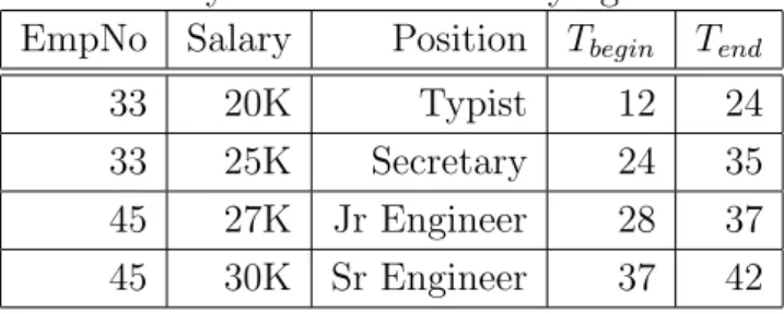
Table 3.1 is in TNF, if salary and position are synchronous. In casesalary
and position are not synchronous there would be time dependence and table
3.1 would have to be normalized, resulting in two relations shown in table 3.2.
Table 3.1: Synchronous time-varying attribute
EmpNo Salary Position Tbegin Tend
33 20K Typist 12 24
33 25K Secretary 24 35
45 27K Jr Engineer 28 37
Table 3.2: Time normalization (following [Tansel et al., 1993](p 97))
EmpNo Salary Tbegin Tend
33 20K 12 24
33 25K 24 35
45 27K 28 37
45 30K 37 42
EmpNo Position Tbegin Tend
33 Typist 12 24
33 Secretary 24 35
45 Jr Engineer 28 37
45 Sr Engineer 37 42
3.3
Research status
Storing time varying information in databases has been done for decades and there has been research activity in this area for quite some time [Snodgrass, 1990]. Since 1998 temporal support is indeed a part of SQL standard. SQL3
supports a serie of temporal data types like DATE, TIME, TIMESTAMP. Further
the notion of a table with temporal support is supported. A table can have
valid-time support, transaction-time support, or both (bitemporal support) [Snodgrass, 1998]. Nevertheless neither the commercial database management
systems (DBMS) such as Oracle, Sybase, Informix and O2[Steiner, 1998] nor
the open-source projectsPostgreSQLandMySQLhave fully implemented this.
The data types DATE, TIME and TIMESTAMP are widespread in most DBMS,
but native (bi)temporal table support or a temporal query language is only
3.3.1
Temporal Query Languages
A notable part of the research in temporal databases focuses on the develop-ment of temporal query languages.
While conventional SQL lacks from featuring support for temporal data, researchers proposed many temporal query languages, to simplify and opti-mize manipulation of temporal data. Temporal query languages reduce the amount of database code needed for temporal data queries by as much as a factor of three in comparison to the standard SQL query language [Jensen, 2000](preface)
We present a selection of query languages extending SQL:
3.3.1.1 TempSQL
TempSQLis a extension of SQL with much more expressive power than
conven-tional SQL. For SELECT statements the additional expression WHILE simplifies
temporal queries tremendously. [Tansel et al., 1993](page 38) A query “Give
managers of John” is expressed in TempSQLas follows:
S E L E C T name , m a n a g e r
W H I L E emp . d e p t = m a n a g e r . d e p t F R O M emp , m a n a g e m e n t
W H E R E n a m e = J o h n
The WHILE clause limits the time range of the result set to managers, who
were in chargewhileJohn was actually working in their department. Managers
running the departments John worked in before or after he worked there are excluded.
3.3.1.2 TSQL
TSQL is also a superset of SQL. [Tansel et al., 1993](page 99) TSQL has
the additional constructs like the WHEN and TIME-SLICE clause. Using the
WHEN clause comparison of time intervals becomes very easy. A query “Find
the manager of employee 23 who immediately succeeded manager Jones” is
S E L E C T B . mgr F R O M m a n a g e m e n t A , m a n a g e m e n t B W H E R E A . e m p l o y e e n u m = B . e m p l o y e e n u m AND A . e m p l o y e e n u m =23 AND A . m a n a g e r = ’ J o n e s ’ W H E N B . I N T E R V A L F O L L O W S A . I N T E R V A L 3.3.1.3 HSQL
The Historical Query Language supports real time1 databases. ([Tansel et al.,
1993](page 110)
HSQL supports the definition of historical relations.
C R E A T E S T A T E T A B L E emp ( ENO C H A R ( 1 0 ) ,
SAL D E C I M A L (5) , U N I Q U E ( ENO ) )
W I T H T I M E G R A N U L A R I T Y D A T E
This statement creates two relations in the background, namely
CURRENT-EMP(ENO, SAL, FROM, TO) and HISTORY-EMP(ENO, SAL, FROM, TO). Data
manipulation operations are performed on the virtual relationEMPand passed
on to the CURRENTrespectively HISTORY relations.
3.3.1.4 TSQL2
TSQL2, is a temporal extension to the SQL-92 language standard. It comes
from a different group of researchers thanTSQL. [Snodgrass et al., 1994],[Jensen,
2000](Part I+II)
For example creating a table with valid time timestamped tuples is done
by adding an option AS VALID STATE to the table definition statement:
C R E A T E T A B L E Emp
( ID S U R R O G A T E NOT NULL ,
N A M E C H A R A C T E R ( 30 ) NOT NULL , S a l a r y D E C I M A L ( 8 ,2 ) )
AS V A L I D S T A T E ;
Inserting a tuple looks as follows:
I N S E R T I N T O Emp
V A L U E S ( NEW , ’ J o h n ’ , 8 5 0 0 0 )
V A L I D P E R I O D [ 2 / 1 / 2 0 0 2 - 1 / 3 1 / 2 0 0 7 ] ;
And a query “Who had the same salary for the longest total time?” in
TSQL2 looks as follows: S E L E C T S N A P S H O T E2 . N A M E F R O M Emp ( ID , S a l a r y ) as E1 , Emp ( ID , N a m e ) as E2 ( S E L E C T MAX ( C A S T ( V A L I D ( E ) AS I N T E R V A L DAY ) F R O M Emp ( ID , S a l a r y ) ( P E R I O D ) AS E ) AS E3 W H E R E E2 . ID = E1 . ID
The list TQuel, are extension to the relation data model. HRDM (Historical Relational Data Model)
3.3.2
Temporal joins
Joins in temporal databases are an issue because of the following reasons: First, conventional techniques are designed for the evaluation of joins with equality
predicates rather than the inequality predicates prevalent invalid time queries.
Second, the presence of temporally varying data dramatically increases the size of a database.[Gao et al., 2003]
Researchers have proposed new join operators for temporal databases like
temporalCartesian product,time join,TE-join,natural time join,
in-tersection join, union join, etc.
We present an example for an application of the temporal Cartesian
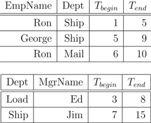
product operator. Consider a database with two relations shown in table 3.3.
Table 3.3: Temporal join example following [Gao et al., 2003](p 97))
EmpName Dept Tbegin Tend
Ron Ship 1 5
George Ship 5 9
Ron Mail 6 10
Dept MgrName Tbegin Tend
Load Ed 3 8
Ship Jim 7 15
A query “Show the names of employees and managers where the employee
worked for the company while the manager managed some department in the
company” would lead to a complex query using conventional SQL. A join
operator performing a temporal Cartesian product simplifies this task. The
resulting relation is shown in table 3.4.
Table 3.4: Result of temporal Cartesian product
EmpName Dept Dept MgrName Tbegin Tend
Ron Ship Load Ed 3 5
George Ship Load Ed 5 8
George Ship Ship Jim 7 9
Ron Mail Load Ed 6 8
Ron Mail Ship Jim 7 10
3.3.3
Temporal indexing techniques
Another subfield of temporal database research is about indexing techniques. Since temporal normalization leads to data models with many fragmented relations, database performance becomes an issue.
Like most indexing structures, the desirable properties of a temporal index include efficient usage of disk space and speedy evaluation of queries.[Ooi et al.,
1998]. Since bitemporal records can be viewed as bounded planes in a 2-dimensional space, indexing techniques from spatial databases can be adapted.
[Jensen, 2000](chapter 36) proposes an extension of theR*-tree, calledGR-Tree
supposed to be faster than the original R*-tree.
3.4
Approaches
This section introduces some approaches for designing temporal database mod-els found in literature focusing on approaches that build bitemporal database models upon conventional relational databases.
3.4.1
Concepts of “now” and “infinity”
In a temporal database we want to be able to store information like “Fact X
is valid since ’01 Jan 2005’ until now”. But“now” is not a constant value but
rather an ever changing variable. “now” is expressed in SQL as CURRENT
-TIMESTAMP within queries, but for storing the information behind “now” in the database, a concept is needed.
Some DBMS feature a database-resident variable, such as “now”,
“until-changed” (UC), “@” and“-”. Time variables would be convenient but Jensen advices that they would lead to a new type of database, consisting of tuples with variables [Jensen, 2000].
Using a variable “now” is overly pessimistic and limits valid time to the
past[Jensen, 2000]. We can not use“now” to store the information about the
future like “Fact X is valid from ’01 Jan 2010’ until changed” until the year
2010 when it becomes to “Fact X is valid from ’01 Jan 2010’ until now”.
Instead of a variable there are special (non-variable) valid-time values, such as“forever”,“infinity” or“∞”[Jensen, 2000]. With such an approach it does
not matter whether a valid time is in the past or future. Nevertheless Jensen
calls this technique overly optimistic, because the use of a constantforever or
any large date value is always inappropriate and does not model the real world correctly.
3.4.2
Temporal Data Models
We present some relational temporal data models and we confine ourselves to
models supporting bothvalid time andtransaction time, known asbitemporal.
One distinction can be made between models sticking to first normal form
(1-NF) and models not in 1-NF. Related is the distinction betweentuple
times-tamping and attribute-value timestamping. [Jensen, 2000](chapter 6)
Remaining in 1-NF means in this context means, a database is modelled as if it was a snapshot database, following the established normalization rule proposed by [Codd, 1970], and time attributes are added to the tuples. Those
data models remaining within 1-NF withtuple timestamping potentially
intro-duce redundancy because attribute values that change at different times are repeated in multiple tuples.
The non-1-NF models, usually with attribute timestamping avoid redun-dancy. But they are not capable of directly using relational storage structures or query evaluation techniques. The performance of a non-1-NF may degrade. [Jensen, 2000](chapter 6)
3.4.2.1 Trade-off between query performance, complexity and re-dundancy
Modelling a temporal database the same way one would model the equivalent snapshot database and adding time attributes to the tuples is one way to go. Completely decompose the attributes into many relations and timestamp each attribute seperatly is the other extreme.
Consider a database snapshot database consisting of one relation, a timein-variang key, and 5 attributes (table 3.5):
Table 3.5: Example: The snapshot equivalent
Making this database temporal means adding time attributes. One way to do this would be just adding the time attributes to the relation, in other words timestamping the tuples (table 3.6. Assuming all attributes are mutually non-synchronous, changing the value of one attribute would lead to a replication of a whole tuple and the values of the 4 attributes not changed would be saved manifold, resulting in redundancy.
Table 3.6: Example: Relation not in TNF key att1 att2 att3 att4 att5 Tbegin Tend
Time normalizing the given relation leads to 5 relations shown in 3.7. The space needed to store one version of a tuple is higher in fact, but as the at-tributes values change asynchronously over time, the storage space needed becomes less, because data is not stored redundantly, as in the non-TNF rela-tion.
Table 3.7: Example: Time normalized key att1 Tbegin Tend
key att2 Tbegin Tend
key att3 Tbegin Tend
key att4 Tbegin Tend
key att5 Tbegin Tend
3.4.3
Separation of history relation
The currently valid tuples and the historic tuple could theoretically be stored in the same table. In practice, the currently valid tuples are usually stored in acurrent table and the historical tuples are kept in separate table called audit
orhistory table. Referenz
Our approach
This chapter covers a detailed presentation of our approach of building a bitem-poral database.
Our bitemporal data model is based on a conventional relational database.
For the sesam subject management database the data volume, the number of
tuples as well as the update frequency of the time-varying attributes are on a manageable scale. Therefore our approach focuses not primary on scalability and performance issues, but on a wieldy complexity.
For instance we do not completely time-normalize the relations as proposed by Navathe and Ahmed[Tansel et al., 1993], but rather keep the attributes together in as few relations as possible.
Furthermore we introduce a layer hiding the partly time-normalized rela-tions for the application by providing updatable views.
4.1
Our “now” concept
According to Jensen, there is no variable “now” in conventional databases, only in temporal databases[Jensen, 2000].
Since we build our approach on a conventional database we are interested in developing a concept without a variable.
In order to store information like “Fact X is valid since ’01.01.2005’ until
now” or “Fact X was valid since ever until ’01.01.2005’ ” we do not use a
variable but we use the lower and upper boundaries of the value range of the timestamp data type of our DBMS. The upper boundary of timestamp is called
infinity, the lower boundary-infinity.
Like in math, we call the interval [−inf inity, inf inity] open. Let d1 and
d2 be date values with condition −inf inity < d1 < d2 < inf inity. Then the
intervals [−inf inity, d] and [d, inf inity] are half-open, and [d1, d2] is a closed
interval.
For a fact associated with a half-open interval in the transaction time
do-main, this means it is a current fact. Aclosed interval in thetransaction time
domain implies that a fact is historic. There is no open interval in the
trans-action time domain, since there is always a lower bound, representing the date when a tuple was entered into the database.
Valid time intervals are either closed intervals, with a determined begin
and end, or they come up to a half-open interval with only one determined
boundary, and if neither the begin and end are known, it results in an open
interval.
4.2
Keys
There are special issues concerning keys we have to deal with in a bitemporal database. There are two aspect about keys we do not have in a conventional database: First, in temporal databases an object of the real world is not rep-resented by one object in the database, but by multiple versions of the object. Second, we assume all attributes are subject to modification, even the natural key of an object. Since each object is referenced by other tuples, namely its history tuples, updates of the key attributes would lead to a chain reaction of updating references.
For these reasons it is accurate to have an artificial key representing the
objects of the real world we call static id, also known as timeinvariant key
timevary-ing version we call timevarying id. So the unique identifier for each currently
valid version of an object is a key composed of its static id and none, one or
several timevarying ids. The key of the historic objects are composed of the
key of its current object plus the transaction time.
4.3
Time normalization
4.3.1
Valid time domain
For the domain of valid time, we follow the proposed time-normalization of
Navathe and Ahmed[Tansel et al., 1993](p 97) only in parts. As seen in section
3.4.2.1 in an application, were all attributes areasynchronous from each other,
time-normalization leeds to decomposition of the relations. Strictly following the rulse of time-normalization would lead to a data model were the number of relations equals the number of attributes. Such a fragmented data model degrades performance and becomes confusingly complex.
In our approach relations are only split to a minimum extent, so the com-plexity of the data model remains low, and queries perform well. In most cases a relation is split into a static one, only with time-invariant attributes, and one or two time-varying relations.
Besides this model reduces at least a part of the redundancy, compared to just timestamping the snapshot model, it has the advantage, that static keys are in static relations, and therefore they are unique keys and they can be referenced by other relations.
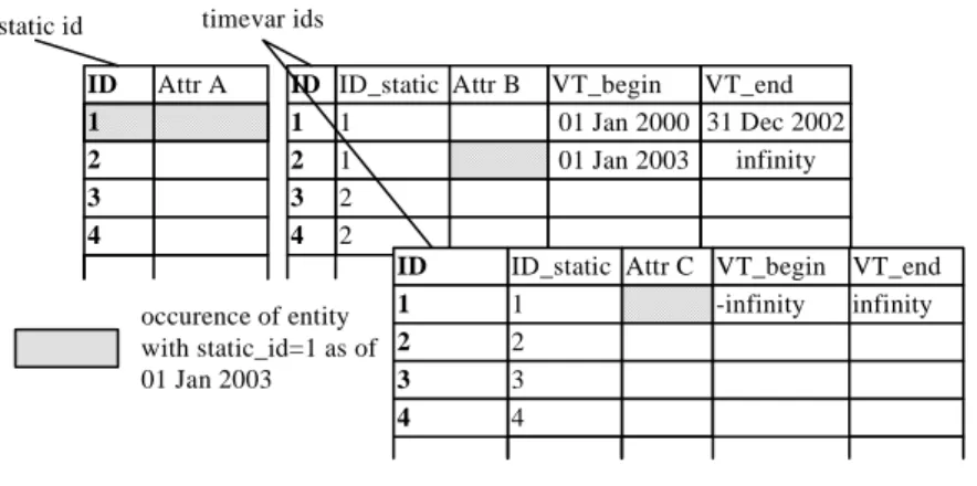
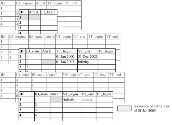
Figure 4.1 illustrates an example of how an object(key, A, B, C)is split
along the columns into a static and two time-varying relations for the valid
time domain. Attribute A is a static one while B and C are time-varying.
The different versions of the object can be assembled by joining toghether the
tuples in the three relations with the samestatic id and overlappingvalid time
Attr A ID 1 2 3 4 Attr B VT_begin 01 Jan 2000 01 Jan 2003 VT_end 31 Dec 2002 infinity ID_static 1 1 2 2 ID 1 2 3 4 Attr C VT_begin -infinity VT_end infinity ID_static 1 2 3 4 ID 1 2 3 4 occurence of entity with static_id=1 as of 01 Jan 2003
static id timevar ids
Figure 4.1: Split into static and time-varying relations
4.3.2
Transaction time domain
In the domain of transaction time (TT), tuples are divided into current and
historic data sets. We call a relation with currently valid tuples current
rela-tion, the one with the historic tuples history relation.
Each tuple’s T Tbegin value is a certain date value in the past. If the T Tend
is also a certain date value in the past, it means that such it is historic. Such a tuple belongs either to a deleted data set or it was overwritten. Storing current and historic tuples in the same relation is one possibility. But there are some reasons to separate them. Since current tuples are typically accessed much more frequently than historic tuples, it makes sense to keep them in a separate table for performance reasons. The number of historic tuples can be much higher than the number of current tuples.
Another point supporting a separation of current and historic data sets is that current tuples are referenced by other current tuples and therefore the key of an object should not change. As introduced in section 4.2 in our
approach, current tuples always have a primary key (id), while the historic
tuples’ primary key is composed of the primary key of the current relation
plus thetransaction time: (id, ttbegin). In our application, references among
historic tuples are usually not needed. Historic tuples are typically accessed via their current version.
Since in the current relation all tuple’s T Tend value is equal to now, this
attribute can be omitted.
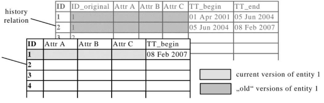
ID 1 2 3 4 ID_original 1 1 2 2
Attr A Attr B Attr C TT_begin 01 Apr 2001 05 Jun 2004 TT_end 05 Jun 2004 08 Feb 2007 TT_begin 08 Feb 2007 ID 1 2 3 4
Attr A Attr B Attr C
current version of entity 1 „old“ versions of entity 1 history
relation
Figure 4.2: A database consisting of a current relation (black) and a history
relation (grey).
One might argue that in the domain ofvalid time a separation of currently
valid and formerly or future data sets would make sense for the same reason.
However for thevalid time domain there exist data sets that are already in the
database but will become valid in the future. With such a model one would always have to check whether a data set becomes valid at this moment and if so, move it to the current relation. Such a permanent monitoring would be rather hard to handle. On the one hand implementing such a mechanism would be quite complex compared to our solution. On the other hand permanently monitoring a sizable part of the database would lead to performance issues.
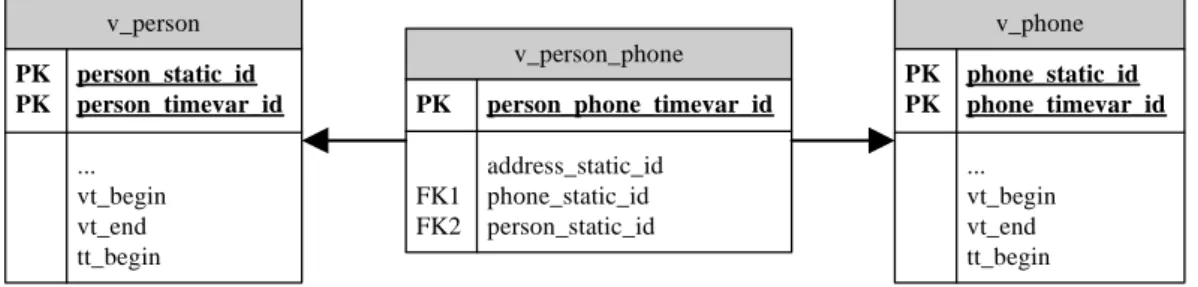
4.3.3
Bitemporal domain
Combining the two approaches for valid time and transaction time leads to
the picture illustrated in figure 4.3.
Each of the relations resulting from the time-normalization (black) features a history table (grey). One object is identified by its static primary key. The different versions have a key composed of the static key and the time-varying keys.
A relation of the snapshot model results in 2, 4, or 6 relations in the bitemporal model using our approach.
occurence of entity 1 as of 01 Jan 2003 Attr A ID_original 1 2 3 4 TT_begin ID 1 2 3 4 TT_end Attr A ID 1 2 3 4 TT_begin
Attr B VT_begin VT_end ID_static 1 1 3 4 ID_original 1 2 3 4 TT_begin ID 1 2 3 4 TT_end Attr B VT_begin 01 Jan 2000 01 Jan 2003 VT_end 31 Dec 2002 infinity ID_static 1 1 2 2 TT_begin ID 1 2 3 4 Attr C VT_begi n VT_end ID_static 4 4 3 4 ID_origi nal 4 4 5 6 TT_begi n ID 1 2 3 4 TT_end TT_begin Attr C VT_begin -infinity VT_end infinity ID_static 1 2 3 4 ID 1 2 3 4
Figure 4.3: Our approach of a bitemporal database
4.4
Intermediate layer
The main disadvantage of time-normalization is that the application program-mer has to deal with a complex and fragmented data model. In order to reduce this drawback, our approach introduces a layer between the split relations and the application. This layer consists of updatable views. The application per-forms INSERT, UPDATE and DELETE operations on these views as if they were database tables.
An INSERT statement on such a view can have two different meanings. In one case, a new object is inserted into the database. Thus tuples have to be inserted into the static and time-varying relations. In the other case, if an existing primary key of the static relation is given, it is about inserting a new time-varying tuples. In this case, there is no insert into the static relation, but potentially an update on an existing tuple of the static relation.
always possible or might not have a definite implication. For instance updating aggregated values is not possible or updating underlying relations without its key might cause nondistinctive behaviour. Therefore the views to be updated in our approach have no aggregations and must comprehend a unique key of the underlying relations.
With this layer, a data model is presented to the application programmer with the complexity level of the equivalent snapshot database. Indeed, joining toghether the decomposed relations could also be done on application level. But then every application accessing the database would have to implement the same functionality itself. We think this is a strong argument to implement this layer on the database.
4.5
Interval overlaps
In section 3.2.4 we introduced a new kind of constraints occurring in temporal
databases. If valid time intervals of a certain object shall not overlap, a new
kind of database constraint is needed.
Since the valid time interval boundaries are typically entered by the users,
the database has to assure the compliance with the interval constraints. One strategy could imply that inserts or updates leading to a constraint violation are refused by the DBMS. This would lead to a lot of manual work for the users since the validity intervals of existing data set would have to be adapted before.
The strategy in our approach assumes that the currently inserted or up-dated data set has priority and the other existing tuples have to make room for it.
Figure 4.4 lists all possible constellations of one existing interval x and a
new intervaly with priority.
In case (1) and (13) the existing interval is not affected by the insertion of
y since the intervals do not overlap.
Whether case (2) and (12) require action depends on the convention whether the begin of one interval can be equal the end of another interval or not. If such a convention applies, case (2) and (12) represent an overlap, otherwise not. Our approach suggests a convention that the boundaries of two meeting intervals have to be distinct from each other. The end of the preciding interval needs to be smaller than the beginning of the succeeding. We define a mini-mum difference, which is the smallest possible interval length of the given data
type. This interval is called “chronon”, and its actual lenght is depending on
the data type of the used DBMS.
Thus in cases (2), (3) and (4) the interval x’s begin would have to be set
to yend + 1“chronon00. In case (8), (11) and (12) xend has to be pruned to
ybegin−1“chronon00.
In a situation of type (9), intervalx has to be split into two intervals. One
with axbegin unchanged but xend set toybegin−1“chronon00. A second interval
has xbegin :=yend+ 1“chronon00 and a unchanged xend.
In cases (4), (5), (7), (8) the existing data set is replaced because the new one overlaps it completely.
Recapitulatory, the 13 cases of overlapping can be categorized into the following situations:
• (2), (3) and (4): xbegin is postponed
• (10), (11) and (12): xend is preponed
• (9): x is split
• (4), (5), (7), (8): the old entry is replaced.
For our application we assume that the standard operation has the following pattern: For example, a person’s name’s validity end will usually be set to
+infinity. When a new name is entered, the old name’s validity ends just
One can consider warning the user if a gap in validity results. For our example of person’s names this would be useful since having a time period when a person does not have a name would be an unwanted situation. This problem depends on the kind of information to be stored.
4.5.1
The “main address” problem
A very similar kind of constraint concerning interval overlaps is the following: Overlapping of the tuples in a relation shall be allowed, but for certain values, there shall be no overlapping.
Such a constraint in an application could be that a person can have several addresses whose validity can overlap arbitrarily. But at every point there can
be only onemain address.
One possibility is to model the relationship between persons and addresses with two relations, one for the main address and one for the others. Then the same rule for overlapping as described in the previous section could be applied for the main address relation and no special action would be needed for the other relation. But maintaining the same kind of relationship in two distinct relations has also drawbacks. If for example a person-address relationship already exists and later becomes a main address, the administration effort would be much higher than have all the relationships in one database table.
Therefore our approach suggests to maintain one table for person-address relationships. A constraint is needed which assures that if an address is set as
the main address, the completely overlapped addresses need to be set to
non-main, and the partially overlapped addresses have to be split into an interval
when they aremain and a non-main interval.
Figure 4.5 shall illustrate the problem of inserting a new main
person-address relationship where already exist main person-addresses. The left side is the situation before inserting the new relation, while on the right side is the situ-ation after inserting. The interval about to insert (dotted) partially overlaps an existing interval and completely overlaps a second one. The partially
Implementation
This chapter describes the design and development of the bitemporal database and the Java client.
5.1
Requirements
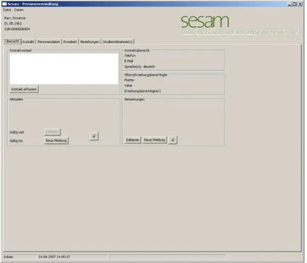
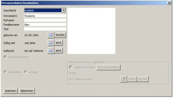
The sesam study requires a software client with the capability to enter, view and modify data about persons, more precisely study subjects and employees. The information to be maintained about persons includes personal data like
name,gender,date of birth, etc.,postal addresses,e-mail addresses and phone
numbers. For study subject further personal details about the persons are
stored like languages, life dates and special annotations and announcements.
Special annotations include notes about individual restrictions like disabilities.
Annotation inform about special circumstances like for example the death of a family member.
Since a significant part of the sesam research includes the studies of
par-ents and grandparpar-ents, relations among study subjects are represented in the
database. Besides themother,father,legal representative and grandparents of
the study subject there are also relationships between the adults namely
participation status in the project itself, as in the sub-studies is maintained and typically changes during the more than twenty years the project lasts.
For employees hiring date, jobrole and the core studies they are working at
are stored in the database.
5.1.1
Given systems
Since the application for subject management of sesam is part of a greater
project including other databases connected to it, the project managers laid down to use one single database product to be used by all applications. There exist Database Management Systems designated for temporal and bitemporal
data models, like for exampleTimeDB[Schmidt, 2005], but they are all niche
products whose durability is not assessable. Moreover many of the standard features of a modern conventional DBMS are not available in these specialized systems. Therefore it was decided to use a widely established relational DMBS
PostgreSQL.
The Database Management System as well as the Programming Language
are already established within the sesamDB project. The DBMS is the open
source database PostgreSQL (Version 8.x). The client application is build
with Java and the graphical user interface is made with the Standard Widget
Toolkit (SWT). The use of SWT makes it possible to run the application on
different operating system because SWT accesses the user-interface facilities
of the operating systems on which it is implemented [SWT, 2007].
5.1.2
Client requirements
The primary aim of the client application is to provide an intuitive graphical user interface which allows the users to enter, view and modify data about study subjects and employees. Besides accessing the current information there is also the possibility to view the history of data modifications. One can see who when updated a data set which helps if investigations are required.
client. Temporal operations like historization, and checking temporal interval constraint should be handled by the database.
5.1.3
Database requirements
All entities and relations time varying in the real world are modelled as such in the database. All data changes have to be traceable, which implies that audit tables are required for all database tables. This includes that the modifier is stored together with each tuple.
This section describes the requirements of the software. Some exemplary use cases are described detailed.
5.2
Architecture
Figure 5.1: The architecture
On the lowermost layer are the database tables. Some of the application logic, like e.g. the “historization” of data, is implemented with triggers. By having the historization functionality at this level, all applications writing to the database can benefit from it. They do not have to care about historization of their data manipulations.
In the case of non-split relations, the application performs its operation directly on the database tables (pictured by the right arrow). If bitemporal relations are split into multiple tables, they are joined together to views. Thus the fragmented relations are hidden to the application layer. These views are updatable and the application performs data manipulation operations on
them (pictured by the left arrow). INSTEAD OF RULEs, as they are called in
PostgreSQL, are responsible to remit the operations on the views to the tables.
In other DBMS, e.g. Oracle this procedures are calledINSTEAD OF TRIGGERs.
The advantage of having this layer of views is that applications do not have to maintain various relations. The consistency of the data spread over the various relations is assured by the database. Particulary with regard to
that several applications might access the database, a lot of implementation work only has to be done once.
The upper part of figure 5.1 illustrates the Java application. The
persis-tency of Java objects is done using the Hibernate framework. Hibernate is
widespread, easy to use and distributed under theGeneral Public License
[Hi-bernate, 2007]. A similar framework would have beeniBATIS by the Apache
Software Foundation By means of both frameworks, plain Java Objects (
PO-JOs) are are mapped to their database equivalent via XML mappings. The
persitency framework loads tuples from the database, creates a POJO with and save them.
The actual Java application is responsible to display the persistency objects on the (SWT) graphical user interface and remit data manipulations on them to the persistency framework.
5.3
Database
This section describes the modelling and implementation of the database. When designing a conventional snapshot database one entity or relationship is normally modelled as one database relation.
In our bitemporal database, an entity that would be modelled as one rela-tion in a snapshot database, is split into several relarela-tions and requires triggers for historization. In order to hide the complexity of the underlying database model, views are provided that join toghether the split relation.
Entity_X_static PK id ... tt_begin modified_by modifier_comment Entity_X_timevar PK id FK1 Entity_X_static_id ... vt_begin vt_end tt_begin modified_by modifier_comment V_Entity_X Entity_X_static_id Entitiy_X_timevar_id ... ... vt_begin vt_end tt_begin modified_by modifier_comment Entity_X_static_hist PK id Entity_X_static_id ... tt_begin modified_by modifier_comment deleted Entity_X_timevar_hist PK id Entity_X_timevar_id Entity_X_static_id ... vt_begin vt_end tt_begin modified_by modifier_comment deleted V_Entity_X_static_hist Entity_X_static_id ... tt_begin modified_by modifier_comment deleted V_Entity_timevar_hist Entitiy_X_timevar_id ... vt_begin vt_end tt_begin modified_by modifier_comment deleted V_Entity_X_hist Entity_X_static_id Entitiy_X_timevar_id ... ... vt_begin vt_end tt_begin modified_by modifier_comment deleted
historize trigger historize trigger application access (SELECT, INSERT, UPDATE, DELETE) application access (SELECT only) rules rules
Figure 5.2: Overview of database model
Figure 5.2 illustrates the collaboration of relations, views, rules and
trig-gers that are necessary for a split time-varying entity Entity X. Relations
En-tity X static and Entity X timevar store the current data while Entity -X static histandEntity X timevar histstore the historic data. Relations
Entity X static and Entity X timevar are joined together and form view
manipulations can be performed on it as if it were a database table. Rules are converting the data manipulation commands and propagating them to the
relations Entity X static and Entity X timevar.
Each modification of tuples in relations Entity X static and Entity X
-timevar causes firing a historize trigger. If a tuple in one of the current relations is updated, it is copied to the dedicated history relation before the
update is performed. In case of a deletion, a tuple is removed from thecurrent
relation to the history relation. A boolean attribute deleted of the history relation indicates whether an tuple was deleted.
Eachcurrent relation has a dedicatedhistory relation. Each of this pair of
relations is combined to a read-only view. Entity X static and Entity
-X static hist form the view V Entity X static hist in our illustration.
V Entity X static hist and V Entity X timevar hist form the basis for
V Entity X hist.
The reason for these intermediate views where current and history data are
combined is that in V Entity X hist current tuples are joined together with
historic tuples. Consider an entity is split into static and timevar relations. An update on this entity might affect only the time varying part of the entity. Thus no history entry exists for the static part although it is part of a historic version of the entity.
The proceeding subsections explain the relations, views, rules and triggers more detailed.
5.3.1
Common conventions
The following common conventions affect all types of relations: For all
rela-tions exists an identification column id of type bigint. The values for id
are generated by calling a sequence nextval(’seq Entity X static id’).
This practice of using a generated number as primary key is widespread. It is especially convenient when inserting tuples into multiple related tables,
be-cause one knows theid of a tuple before inserting it. The next value from the
Or the value for id is empty in the insert statement and the default value
defined for theid attribute calls the sequence.
Besides the primary key column id there are columns tt begin and
mod-ified by in order to keep track of from whom and when a tuple was entered, edited or deleted. The modifier data is set by a trigger. Additionally the
field modifier comment is there for entering any comments about the reason
a tuple was updated or deleted.
5.3.2
Static relations
For entities with static attributes, a static relation of the following pattern
exists: C R E A T E T A B L E E n t i t y _ X _ s t a t i c ( id b i g i n t NOT N U L L D E F A U L T n e x t v a l ( ’ s e q _ E n t i t y _ X _ s t a t i c _ i d ’ ) , /* s t a t i c a t t r i b u t e s */ ... t t _ b e g i n t i m e s t a m p NOT N U L L D E F A U L T now () , m o d i f i e d _ b y text , m o d i f i e r _ c o m m e n t text , C O N S T R A I N T E n t i t y _ X _ s t a t i c _ p k e y P R I M A R Y KEY ( id ) ) ;
In order to track data manipulation on this table a trigger function is
implemented. The following snippets in the historize trigger function are
responsible to write to the history table: For the case of deletion:
... I N S E R T I N T O E n t i t y _ X _ s t a t i c _ h i s t ( E n t i t y _ X _ s t a t i c _ i d , /* s t a t i c a t t r i b u t e s */ ... m o d i f i e d _ b y , m o d i f i e r _ c o m m e n t , t t _ b e g i n , tt_end , d e l e t e d ) V A L U E S ( OLD . id , /* s t a t i c a t t r i b u t e s */ OLD . ... OLD . m o d i f i e d _ b y , OLD . m o d i f i e r _ c o m m e n t , OLD . t t _ b e g i n , c u r r e n t _ t i m e s t a m p ,
’ t r u e ’ ) ; R E T U R N OLD ; ...
For the update case:
... IF /* a n y s t a t i c a t t r i b u t e h a s c h a n g e d */ T H E N I N S E R T I N T O E n t i t y _ X _ s t a t i c _ h i s t ( E n t i t y _ X _ s t a t i c _ i d , /* s t a t i c a t t r i b u t e s */ ... m o d i f i e d _ b y , m o d i f i e r _ c o m m e n t , t t _ b e g i n , tt_end , d e l e t e d ) V A L U E S ( OLD . id , /* s t a t i c a t t r i b u t e s */ OLD . ... OLD . m o d i f i e d _ b y , OLD . m o d i f i e r _ c o m m e n t , OLD . t t _ b e g i n , c u r r e n t _ t i m e s t a m p , ’ f a l s e ’ ) ; NEW . t t _ b e g i n := c u r r e n t _ t i m e s t a m p ; END IF ; R E T U R N NEW ; ...
The history table looks as follows. It contains the same attributes than its
current equivalent, yet the additional attributes tt endand deleted.
C R E A T E T A B L E E n t i t y _ X _ s t a t i c _ h i s t ( id b i g i n t NOT N U L L D E F A U L T n e x t v a l ( ’ s e q _ E n t i t y _ X _ s t a t i c _ h i s t _ i d ’ ) , E n t i t y _ X _ s t a t i c _ i d b i g i n t NOT NULL , /* s t a t i c a t t r i b u t e s */ ... t t _ b e g i n t i m e s t a m p NOT NULL , t t _ e n d t i m e s t a m p NOT N U L L D E F A U L T now () , m o d i f i e d _ b y text , m o d i f i e r _ c o m m e n t text , d e l e t e d b o o l e a n NOT N U L L D E F A U L T false , C O N S T R A I N T E n t i t y _ X _ s t a t i c _ h i s t _ p k e y P R I M A R Y KEY ( id ) )
Notice there is no foreign key constraint from the history to the current table since tuples can be deleted on the current table, but their history remains in the database.
![Table 1.1: Bitemporal database example (following [Wikipedia, 2005])](https://thumb-us.123doks.com/thumbv2/123dok_us/9086727.2400617/8.892.150.766.198.575/table-bitemporal-database-example-following-wikipedia.webp)