A Novel Method for Determining Research Groups from Co-Authorship
Network and Scientific Fields of Authors
Jan Pisanski
University of Ljubljana, Faculty of Arts
E-mail: [email protected], http://oddelki.ff.uni-lj.si/biblio/oddelek/osebje/pisanski.html ORCID 0000-0002-3060-111X
Mark Pisanski
Tomaž Pisanski (corresponding author) University of Primorska, FAMNIT
E-mail: [email protected], https://en.wikipedia.org/wiki/Tomaz Pisanski, ORCID 0000-0002-1257-5376
Keywords: co-authorship network, scientific field, maximal spanning tree, induced subnetwork, pruning of networks, pathfinder network, MST, line-cut
Received:March 9, 2020
Large networks not only have a large number of vertices but also have a large number of edges. Although such networks are generally sparse they are usually difficult to visualise, even locally. This paper considers the case where large weights on edges represent similarity between the corresponding end-vertices. We follow two main ideas in this paper. The first one isnetwork pruning, that is removal of edges that makes the resulting network more manageable while keeping the main characteristic of the original network. The other idea is to partition the network vertex set in such a way that the induced connected components repre-sent groups of network elements that fit together. Furthermore, we assume that the vertices of the network are labeled bytypes. Here we apply our approach to co-authorship network of researchers in Slovenia in order to identify research groups, finding group leaders and the degree of interdisciplinarity of the group. For the network pruning phase we use a MST-pathfinder network and for vertex partition appropriate line-cuts. Each cluster is assigned a distribution of types. In this case, the types correspond to scientific fields, also known as research interests of authors. A measure of interdisciplinarity of research group is derived from such a distribution.
Povzetek: Velika omrežja nimajo le mnogo vozlišˇc, ampak imajo tudi mnogo povezav. ˇCeprav so obiˇca-jno taka omrežja redka, so nepregledna in jih je težko prikazati na sliki, tudi lokalno. Ta prispevek obrav-nava omrežja, pri katerih velike vrednosti uteži na povezavah pomenijo podobnost pripadajoˇcih krajišˇc. V prispevku sledimo dvema glavnima idejama. Prva je klešˇcenje omrežja, to je odstranitev manj pomembnih povezav, zaradi ˇcesar je nastalo omrežje bolj obvladljivo, hkrati pa se ohrani glavna znaˇcilnost prvotnega omrežja. Druga ideja je razdeliti vozlišˇca omrežja tako, da inducirane povezane komponente predstavljajo skupine omrežnih elementov, ki se med seboj prilegajo. Poleg tega predpostavljamo, da so vozlišˇca omrežja oznaˇcena s tipi. V tem prispevku uporabljamo naš pristop k omrežju soavtorstev raziskovalcev v Sloveniji z namenom identifikacije raziskovalnih skupin, iskanja voditeljev skupin in stopnje interdisciplinarnosti skupine. Za fazo klešˇcenja omrežja uporabljamo usmerjevalno omrežje (MST-pathfinder network), za vozlišˇcno razbitje pa ustrezne reze povezav. Vsaki skupini je dodeljena porazdelitev tipov. Mero inter-disciplinarnosti raziskovalne skupine izpeljemo iz takšne porazdelitve. V tem primeru tipi predstavljajo znanstvena podroˇcja, oz. raziskovalne interese avtorjev.
1
Introduction
In contemporary research community scientists collabo-rate within formal or informal research groups. Identify-ing such groups from data available in various bibliometric networks is an interesting challenge. In this note we pro-pose a method that uses the co-authorship network on the one hand and declared scientific field of authors that can be extracted from some bibliographic databases, on the other.
We propose a theoretical model that uses a network, i.e. graph with weights on edges and labels, called types, on its vertices. We may view labels as scientific fields or sub-fields. Our approach is quite general and can be applied to any weighted network with types. In this paper we apply it to co-authorship networks. Note that scientific fields are sometimes caller research interests.
the number of edges and increase the number of compo-nents, in our case producing research groups. In this step line-cuts are determined. In the second step a collection of induced monotype subnetworks is pruned by applying MST-pathfinder algorithm to further reduce the number of edges while keeping the same connectivity. Our original contribution is combination of both methods and the use of symmetric predicate in the first step; see Algorithm 3. Note that the idea of using MST, pathfinder and MST-pathfinder has been used extensively in the past in variety of contexts of bibliographic and other research[6, 8, 11, 22, 23].
This rough general approach may be refined in several different ways. We present in detail only one such refine-ment and discuss some others in the conclusion. In general, bibliographic networks are very large and allow for a vari-ety of methods for data mining [15], however in this pilot study we focus our attention on a relatively small data set. The data is restricted to Slovenian researchers and is taken from Slovenian bibliographic system SICRIS. Moreover, only researchers that are co-authors of mathematicians are considered.
2
Pruning of co-authorship network
2.1
Co-authorship network
For basics in graph theory, the reader is referred to [4], for network theory, see for instance [3].
Let V be a list of authors from some bibliographic database. We say thatu, v ∈ V are adjacent: u ∼ v, if
uandvare co-authors of a common work from the corre-sponding database. Sometimes we restrict our attention to certain types of works or certain types of co-authorships. Usually only scientific works are considered and the co-authorship graph is computed from a two-mode network
WAcomposed of pairs(w, a), works and authors for each co-authoraof workw. Since binary relation∼is irreflex-ive1 and symmetric it defines a simple graphG= (V,∼)
that we call the co-authorship graph. LetE = {uv ∈
V2|u ∼ v} denote the set of unordered pairs of adjacent vertices ofG. Instead ofG= (V,∼)we may use notation
G= (V, E)to denote the same graph. The graph may be weighted where the weightswon the edges represent the number of joint papers between the two authors. In this way anetworkN = (V, E, w)is obtained. Letw(u, v) de-note this weight. Sometimes, we may consider the weight of co-authorship differently for different numbern(w)of co-authors of workw. LetW(u, v)denote the collection of works co-authored byuandv. For any workwletn(w) denote the number of authors ofw. Then
w(u, v) =|W(u, v)|.
1Sometimes one may use also loops at each vertex. The weight
associ-ated with a loop may depend on the method that the co-authorship graph is constructed. If it is obtained by multiplication of two-mode networks [4] it represent the number of works for a given author. In the fractional approach it may represent the total contribution of an author. Loops are removed if we follow Newman’s approach.
In a fractional approach [2] the weightf(u, v)is defined as:
f(u, v) = X
w∈W(u,v) 2
n(w)2.
In case of Newman’s normalization the weight is:
f(u, v) = X
w∈W(u,v)
2
n(w)·(n(w)−1)
A networkN is a weighted graphN = (V, E, w), where
w:E→Ris theweight function. In our case it is positive and the value0means there is no edge betweenuandv.
A graphG = (V,∼) is transformed into the network
N = (V, E, a), wherea(u, v) = 1for all adjacent pairs of verticesu∼v. The same bibliographic database can pro-duce at least three types of networks for the weight func-tionsa, w, f,defined above:
1. (V, E, a), thebinary case,
2. (V, E, w)thestandard case, and
3. (V, E, f), thefractional case.
Algorithm 4Prune the networkN = (V, E, w), n=|V|, m=|E|
1: Partition the edge set E into subsets Ei with equal
weights:Ei={e∈E|w(e) =wi}.
2: Order the parts in descending order of weightsw1 >
w2> . . . > wk 3: foru∈V do
4: Su={u} 5: F =∅
6: fori= 1,2, . . .,kdo
7: Fi=∅
8: fore=uv∈Eido
9: LetSu, Svbe the corresponding sets. 10: ifSu6=Svthen
11: AppendetoFi.
12: fore=uv∈Fido 13: ifSu6=Svthen 14: Su=Sv=Su∪Sv 15: ExtendF byFi
16: returnsubnetworkP r(N) = (V, F, w).
There is another aspect that we have not considered in this paper. Namely, the weight of an edgee=uvbetween two authors uandv may depend also on the total num-ber of papers authored by each of the two authors. In this case we may modify the network to allow loops and define
w∗(u, v) = w(u, v)foru6=vand letw∗(u) = w∗(u, u) denote the total number of papers havinguas an author. Note that in generalw∗ cannot be computed directly from
their applications to bibliographic data can be found, for instance in [3].
2.2
Pruning networks
In the analysis of large networks, dense networks present a challenge. Usually one tends to partition the set of vertices and investigate the induced networks on such parts. In [3] one may find a variety of concepts that are useful in such analysis, e.g. cuts, islands, etc. Nevertheless, such subnet-works may be dense again and the role of particular vertices is not clearly visible. For this reason we prune the original networkN = (V, E, w)by appropriately selecting a subset of important edgesE0 ⊂ E. Ifw0 denotes the restriction of w onE0, the pruned subnetworkN0 = (V, E0, w0)is obtained.
In case of co-authorship networks large weights indicate close collaboration between authors. When considering re-search groups one may assume strong collaboration within each group. Hence, in such a case a natural approach to pruning would be to remove all edges of lesser weights, while keeping the same connected components. A pos-sible solution is given by the well-known maximum cost spanning tree. More precisely, in case of a disconnected network the resulting graph is a maximum cost spanning forest.
However, the problem with a maximum cost spanning forest is that, in case when several edges have the same weights, the forest may not be unique. We use a Kruskal-like algorithm that produces a unique pruned network. Algorithm 1 is almost identical to the MST-pathfinder algorithm of [14] and produces the pathfinder network
P n(∞, n−1); for discussion and various aspects see also [19, 5, 20].
It is not hard to see, that the following is true:
Theorem 1. The network N0(V, F, w)is uniquely deter-mined from the original network. If all weights are positive, the connected components are the same as in the original network.
Theorem 2. If all weights inN(V, E, w)are distinct, Al-gorithm 1 produces the (unique) maximum cost spanning forest. On the contrary, if all weights are the same no edge is discarded.
Moreover, we easily compute the running time of Algo-rithm 1.
Theorem 3. The time complexity of the above algorithm is
O(mlogm).
In fact, the time complexity is the same as for Kruskal’s algorithm[10]. The sorting and partitioning takes O(mlogm)steps. There are two loops, each withO(m) steps, and the time complexity for the UNION-FIND is of lesser order.
By applying this pruning method strong ties among the nodes remain visible.
3
Line-cuts
For further refining the network N(V, E, w) one may choose a parametert > 0, the threshold, or cut parame-ter and prune the edges with weights less thant. In this way the networkNt(V, Et, w)is obtained, where
Et={e∈E|w(e)≥t}.
The choice of parametertdepends on our aims. There are several obvious goals. For instance:
1. We may choose maximal value oftthat guarantees at least a prescribed number of connected components, sayκ.
2. An alternative is to insist that all components have at most prescribed number of vertices, sayν.
We present the basic pruning algorithm; see Algorithm 2. It produces essentially aline-cut, see for instance [3]. The only difference is that we keep isolated vertices.
Algorithm 5 Prune the network N = (V, E, w), given threshold parameter t. Connected components of the re-sulting network are calledline-cuts.
1: F =∅ 2: fore∈Edo 3: ifw(e)≥tthen 4: AppendetoF.
5: returnsubnetworkP r(N, t) = (V, F, w).
In Python, Algorithm 2 can be reduced to a single state-ment:
F = [efore∈Eifw(e)≥t]
4
Pruning networks with vertex
types
Let us assume we are given a finite number of types, or col-orsT, a networkN(V, E, w)and a mappingc :V → T. The structure N(V, E, w, T, c) will be called a weighted network with vertex types. When pruning network with ver-tex types, a connected component consisting of vertices of a single type will be called monotype. Additionally, we will refer to the number of types used in a connected com-ponent as itstype number. The maximum of type numbers of network components is called the type number of the network, In particular, we are interested in networks of low type number, preferably with monotype networks.
– One may insist that all connected components are monotype, or more general that each component has at mostδtypes (colors).
The following basic algorithm (Algorithm 3) for a given network with types removes all edges that have endpoints of different types, or more generally, when they satisfy a symmetric predicateP.
Algorithm 6 Prune the network with vertex types N = (V, E, w, T, c)with given threshold parametertand (sym-metric) predicate P : T2 :→ {>,⊥}. Connected com-ponents of the resulting network are calledmonotype line-cuts.
1: F=∅
2: foruv=e∈Edo
3: ifP(c(u), c(v))andw(e)≥tthen
4: AppendetoF.
5: returnsubnetworkP r(N, t, P) = (V, F, w, T, c).
As we mentioned above the predicateP usually is true if both endpoints are of the same type. However, other op-tions are possible. Namely we may have a similarity im-posed on the predicates andP signifies that two types are sufficiently similar.
We need an algorithm to analyse the network with vertex types; see Algorithm 4. Using these numbers we may select different parameters and re-run this algorithm to reduce the size of the maximal component or alternatively limit the number of different components. We may also insist that all components be composed of a single type.
5
Interdisciplinarity of research
groups and leaders of research
groups
For a given network with vertex types one may perform basic statistics on it. Namely, one may compute absolute frequencies of types on the vertex set.
f(x) =|{v∈V|c(v) =x}|
fi(x) =|{v∈Vi|c(v) =x}|
or relative frequencies
φ(x) =f(x)/n
φi(x) =fi(x)/ni
wheren=|V|andni=|Vi|.
We consider two measures:
r(N) = max{φ(x)|x∈T}
s(N) =|suppφ|=|{x∈T|φ(x)>0}|
and for each component:
r(Vi) = max{φi(x)|x∈T}
s(Vi) =|suppφi|=|{x∈T|φi(x)>0}|
Both measure the diversity of research interests in a re-search group. Ifr(Vi) < 0.5 there is no dominant
disci-pline. Ifr(Vi) = 1, the group is totally homogeneous.
Algorithm 7 Analyse network with vertex types N = (V, E, w, T, c).
1: PartitionV into connected componentsV1, V2, . . . , Vk 2: Letd= max{|Vj|;j= 1,2, . . . , k}
3: forj= 1,2, . . . , kdo
4: b(j) =number of different types inVj. 5: Letγ= max{b(j);j= 1,2, . . . , k}
6: returnnumber of connected componentsk, order of maximal connected componentd, and maximal num-ber of typesγin any component.
One way to define a leader of a research group is to de-termine the vertex of maximal degree in the corresponding network, or even better the sum of weights of edges to the neighbouring vertices. There are two parameters that we are interested in. Letmbe the number of edges of network
Nand letdbe the maximal degree attained at vertexx. Let
d0be the second largest degree. Thenxcan be defined as a leader of the research group, whiledominanceis the quo-tientd/mandabsolutismis defined by expression1−d0/d. Note that it would be also interesting to explore the diver-sity index[21] in this context. However, we will address all of these in a future work.
6
Example
The data used in our experiments was taken from COBIS-S/SICRIS [18] for the works indexed in Scopus [17]. Only papers, where at least one author was a mathematician, were considered. Co-authors that were not registered as researchers in Slovenia were not included. Scientific fields alias research interests, used in Slovenia have three levels. On Level 1 we have:
1 Science 2 Engineering 3 Medicine 4 Biotechnology 5 Social Sciences 6 Humanities 7 Interdisciplinary
1.01 Mathematics 1.02 Physics 1.03 Biology 1.04 Chemistry
1.05 Biochemistry and Molecular Biology 1.06 Geology
1.07 Comp. Intensive Methods and Appl. 1.08 Environment Protection
1.09 Pharmacy
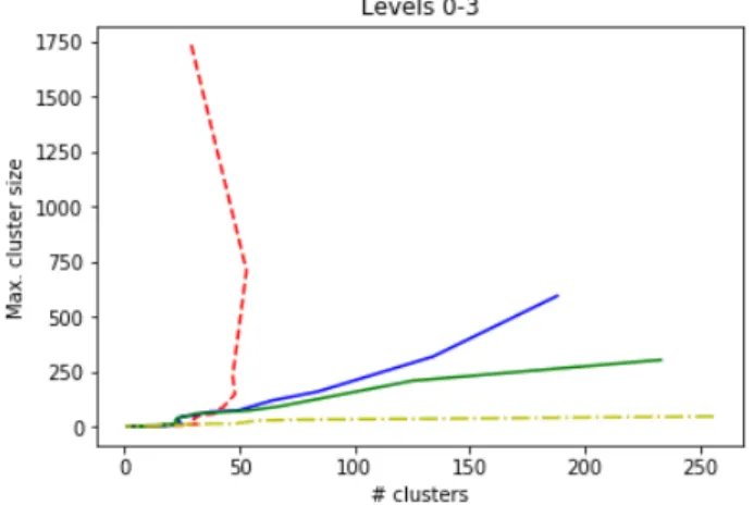
Figure 1: Line-cuts for threshold valuest = 0,1,2, . . .for four different predicates, each depending on the level`= 0,1,2,3. Each predicate depends on the interpretation of equality between two research types. Red –` = 0, blue –
`= 1, green –`= 2and yellow –`= 3.
Finally, the division of Mathematics in the Level 3 is indicated here:
1.01.01 Analysis 1.01.02 Topology
1.01.03 Numerical and Computer Mathematics 1.01.04 Algebra
1.01.05 Graph Theory
1.01.06 Probability and Statistics
Level`may be interpreted as the length of the research interest code that is used to test equality: for` = 0, the string is not used at all, for`= 1only the first characters are compared, for`= 2, the first four characters are com-pared, while for` = 3all seven characters are compared. Different levels can be associated with the suitable choice of predicatePin Algorithm 3. LetP`denote the predicate
applicable to level `. For instance, foru = 1.01.01and
v= 1.01.04P2(u, v) =>whileP3(u, v) =⊥.
Here we give an example of a pruned research group net-work. We intend to perform a thorough analysis on more complete data set elsewhere.
Figures 2 and 3 depict the same research group. The network in Figure 3 is tree-like and is obtained from the
Figure 2: One of several research groups determined by the line-cut fort= 8.
Figure 3: The research group of Figure 2 , pruned by the MST-pathfinder network. Red – Graph Theory, Yel-low – Algebra, Blue – Numerical Mathematics, Green – Mathematics
network of Figure 2 by MST-pathfinder method. Vertex colors denote vertex types: red: 1.01.05, yellow: 1.01.04, blue: 1.01.03 and green 1.01.00. In the database some re-searchers were assigned research interest at level 2, e.g 1.01 (Mathematics). For consistency, we expanded that to level three as 1.01.00. Note that the research group in Figure 3 is composed of two subgroups, one predominantly interested in graph theory and the other in algebra. There is a central triangle connecting the two subgroups.
7
Conclusion
Co-authorship graphs and networks are important in the study of research structure and dynamics; see for instance [7, 9, 12, 1]. Their practical value has first been recog-nised by specialised systems, such as MathSciNet and Zb-Math; see [16, 24]. Including them in more general bibli-ographic systems such as SICRIS [18] would be beneficial for most users. Potential applications are plenty. In this paper we presented only one aspect of such applications. In a recent paper [13] a completely different application is sought, namely, organising talks at a conference in such a way that speakers with similar topics are scheduled at dif-ferent times.
con-sider the function:c:V →T∪ {UNKNOWN}.
Clearly line-cuts refine the vertex partition and apply only within a component. Note that in general one could take different thresholds in different components. In case we intend to have components with given maximal size
ν, then indeed different threshold values may be used. In or future more comprehensive work we intend to ad-dress some further extensions and applications of the MST-pathfinder method as well as some of the parameters that we have introduced.
Acknowledgement
We would like to thank Vladimir Batagelj for useful ad-vice and fruitful discussion. The work of both referees improved the presentation considerably and is gratefully acknowledged. Work of Jan Pisanski is supported in part by the ARRS grants P5-0361 and J5-8247, while work of Tomaž Pisanski is supported in part by the ARRS grants P1-0294,J1-7051, N1-0032, and J1-9187.
References
[1] T. Bartol, G. Budimir, P. Južniˇc, K. Stopar. Mapping and classification of agriculture in Web of Science: other subject categories and research fields may bene-fit.Scientometrics, vol. 109 (2016) no. 2, pp. 979-996. https://doi.org/10.1007/s11192-016-2071-6
[2] V. Batagelj. On Fractional Approach to Analy-sis of Linked Networks, Scientometrics (2020). https://doi.org/10.1007/s11192-020-03383-y
[3] V. Batagelj, P. Doreian, A. Ferligoj, N. Kejžar. Un-derstanding large temporal networks and spatial net-works: Exploration, pattern searching, visualization and network evolution, (2014) John Wiley & Sons.
[4] J.A. Bondy and U.S.R. Murty.Graph theory, (2008) Graduate Texts in Mathematics, 244. Springer, New York.
[5] C. Chen. Science mapping: a systematic re-view of the literature. Journal of Data and In-formation Science, vol. 2 (2017) no.2, pp1-40. https://doi.org/10.1515/jdis-2017-0006
[6] C. Chen, S. Morris. Visualizing evolving net-works: Minimum spanning trees versus pathfinder networks. In IEEE Symposium on Informa-tion Visualization 2003 (2003), pp. 67-74. https://doi.org/10.1109/INFVIS.2003.1249010
[7] A. Ferligoj et al. Scientific collaboration dynam-ics in a national scientific system. Scientomet-rics, vol. 104, (2015), no. 3, pp. 985–1012. https://doi.org/10.1007/s11192-015-1585-7
[8] M. Gallivan, M. Ahuja. . Co-authorship, ho-mophily, and scholarly influence in information systems research. Journal of the Association for Information Systems, vol. 16 (2015) no. 12, 2. https://doi.org/10.17705/1jais.00416
[9] L. Kronegger, F. Mali, A. Ferligoj, and P. Doreian. Collaboration structures in Slovenian scientific com-munities. Scientometrics, vol. 90 (2012), no.2, pp. 631–647. https://doi.org/10.1007/s11192-011-0493-8
[10] JB. Kruskal. On the shortest spanning sub-tree of a graph and the traveling salesman problem. Proceedings of the American Mathe-matical Society. vol.7 (1956) no.1, pp. 48–50. https://doi.org/10.1090/S0002-9939-1956-0078686-7
[11] T. Jacobsen, RL. Punzalan, ML. Hedstrom. Invok-ing “collective memory”: MappInvok-ing the emergence of a concept in archival science.Archival Science, vol. 13(2013)no. 2-3, pp. 217-251.
[12] S. Peˇclin, P. Južniˇc, R. Blagus, M ˇC. Sajko, J. Stare. Effects of international collaboration and status of journal on impact of papers. Scien-tometrics, vol. 93 (2012) no. 3, pp. 937-948. https://doi.org/10.1007/s11192-012-0768-8
[13] J. Pisanski, T. Pisanski. The use of collaboration distance in scheduling conference talks. Informat-ica : an international journal of computing and informatics, vol. 43 (2019) no. 4, pp. 461–466, https://doi.org/10.31449/inf.v43i4.2832.
[14] A. Quirin O. Cordón, V. P. Guerrero–Bote, B. Vargas– Quesada, F. Moya–Anegón. A quick MST-based al-gorithm to obtain Pathfinder networks (∞, n−1),
Journal of the American Society for Information Sci-ence and Technologyvol. 59 (2008) no. 12, pp.1912– 1924. https://doi.org/10.1002/asi.20904
[15] J. Leskovec, A. Rajaraman, and J. Ullman. Mining of Massive Datasets (2014), Cambridge University Press. https://doi.org/10.1017/CBO9781139924801
[16] MathSciNet:
https://mathscinet.ams.org/mathscinet/index.html
[17] Scopus:
https://www.scopus.com/home.uri
[18] SICRIS:
https://www.sicris.si/public/jqm/cris.aspx?lang=eng
[20] HD. White. Pathfinder networks and author cocitation analysis: A remapping of paradigmatic information scientists.Journal of the American Society for Infor-mation Science and Technology,vol. 54 (2003) no. 5, pp. 423-434. https://doi.org/10.1002/asi.10228
[21] Diversity index, Wikipedia,
https://en.wikipedia.org/wiki/Diversity_index
[22] H. Yang, HJ. Lee. Research trend visualiza-tion by MeSH terms from Pubmed. Interna-tional journal of environmental research and public health, vol. 15 (2018) no. 6, 1113. https://doi.org/10.3390/ijerph15061113
[23] SY. Yu. Detecting collaboration patterns among iSchools by linking scholarly communication to so-cial networking at the macro and micro levels. LI-BRES: Library and Information Science Research Electronic Journalvol. 23 (2013) no. 2, pp. 1–13.
[24] zbMATH: