A Novel Normality Test Using an Identity Transformation of the Gaussian Function

(1)

Vol. 4, No. 4, 2011, 448-454

ISSN 1307-5543 – www.ejpam.com

A Novel Normality Test Using an Identity Transformation of the

Gaussian Function

O˘

guz Akbilgiç

1∗

, J. Andrew Howe

2

1_{Department of Quantitative Methods, Istanbul University School of Business Administration,}

Is-tanbul, Turkey

2_{Tennessee Valley Authority, Chattanooga Tennessee, USA}

Abstract. Normality is the most frequently required assumption for statistical techniques. Thus, eval-uation of the normality assumption is the first step of many statistical analyses. Although there are many normality tests in the literature, none dominate for all conditions. This paper introduces a novel normality test, and its performance is compared with some of the other normality tests via a Monte Carlo simulation study. Tests are evaluated according to the Type I error and Power.

2000 Mathematics Subject Classifications: 62E15,62F03

Key Words and Phrases: normality test, Gaussian distribution,probability distributions

1. Introduction

For a given sample dataset, testing whether it follows a normal distribution is a common starting point for many statistical analysis techniques. The literature has many different nor-mality tests using one or more characteristics of the normal distribution function such, as the mean, variance, skewness, kurtosis etc. The Shapiro-Wilk Test[3], Jarqua-Bera[2], and Anderson and Darling Test[1]are some of the most familiar.

In this study, we aim to simultaneously handle all the characteristics mentioned. Logically, the Gaussian function is the unique and most appropriate tool having these characteristics; thus, we have built our test on the Gaussian density function. In section 2, we define a con-tinuous random variable by transforming data using the Gaussian PDF. Then we derive some statistical characteristics like mean, variance, standard deviation and cumulative distribution for this variable. These characteristics are then used to construct a novel normality test, testing the null hypothesis that a given sample data comes from the normal distribution. We show and discuss results from simulation studies in section 3, then finish with some concluding remarks.

∗_{Corresponding author.}

Email addresses:oguzakbilgigmail.om(O. Akbilgiç),ahowe42gmail.om(A. Howe)

(2)

O. Akbilgiç, A. Howe Eur. J. Pure Appl. Math,4(2011), 448-454 449

2. Test For Normality

Let X be a continuous random variable from a normal distribution with mean µ and varianceδ2,X_∼N(µ,δ2). It is known thatX’s density function, called the Gaussian function, and distribution function are shown in (1) and (2), respectively.

f(x) = 1

δp2πe

−1

2((x−µ)/δ) 2

(1)

F_X(t) = 1

δp2π

Z t

−∞

e−12((x−µ)/δ) 2

d x (2)

If we use a transformation to define a new random variable as a function of our dataY = f(X), the mean and variance ofY are obtained by the following process.

E[Y] = E[f(X)] =

Z ∞

−∞ 1

δp2πe

−1

2((x−µ)/δ) 2

· 1

δp2πe

−1

2((x−µ)/δ) 2

d x

= 1

2πδ2

Z ∞

−∞

e−((x−µ)/δ)2d x = 1 2πδ2

Z ∞

−∞

e−12( p

2(x−µ)/δ)2

d x

letu=p2(x−µ)/δ, sodu= p

2

δ d x−→

= 1

2πδ2

Z ∞

−∞

e−u

2 2

δ

p

2du=

p

2π

2p2πδ =

1

2pπδ (3)

E[Y2] = E[f(X)2] =

Z ∞

−∞

{ 1

δp2πe

−1

2((x−µ)/δ) 2

}2_· 1

δp2πe

−1

2((x−µ)/δ) 2

d x

= 1

δ3₂_πp₂_π

Z ∞

−∞

e−32((x−µ)/δ) 2

d x= 1

δ3₂_πp₂_π

Z ∞

−∞

e−12( p

3(x−µ)/δ)2

d x

letu=p3(x−µ)/δ, sodu= p3

δ d x−→

= 1

δ3₂_πp₂_π

Z ∞

−∞

e−u

2 2

δ

p

3du=

1

δ3₂_πp₍₂_π₎·

δp2π

p

3 = 1

2p3πδ2 (4)

Var[Y] =E[(Y−E[Y])2] =E[Y2]−E[Y]2= 1

2p3πδ2−( 1 2pπδ)

2₌ 2−

p

3

4p3πδ2 (5)

Thus, we have µ_Y = 1/(2pπδ), andδ2

Y = (2−

p

3)/(4p3πδ2₎ _{for a random variable} _Y_. Further, we may extract the distribution function of Y as shown here, using the CDF trans-formation method for a random variable. Here we make use of the common standardization notationz= (x−µ)/δ.

F(y) = P Y ≤ y

=P

₁

δp2πe

−1

2((x−µ)/δ) 2

≤ y

=P

e−12((x−µ)/δ) 2

(3)

= P

lne−12((x−µ)/δ) 2

≤lnδp2πy

=P((x−µ)/δ)2_{≥ −}2 lnδp2πy

= P

(x₋µ)/δ_{≤ −}

Æ

−2 lnδp2πy

+P

(x₋µ)/δ_≥

Æ

−2 lnδp2πy

= 2P

(x−µ)/δ≥

Æ

−2 lnδp2πy

=2

1−P

(x−µ)/δ≤

Æ

−2 lnδp2πy

= 2

1−P

z≤ Æ

−2 lnδp2πy

=2

1−Φ

Æ

−2 lnδp2πy

(6)

The complete CDF is

F(y) =







0 y≤0

2

h

1−Φp₋2 lnδp2πy i

0< y < 1

δp2π

1 y_≥ 1

δp2π

. (7)

For the original data, we have X ∈ R_{. With the Gaussian density function, we know that} lim

x→±∞f(X) =0, and

f(µ) = 1

δp2πe

−1

2((µ−µ)/δ) 2

= 1

δp2π.

Thus, our random variable Y has support (0, 1/(δp2π)]. The following calculations show that some features of density functions are satisfied by (7).

F(0) = 2

1−Φ

p

−2 lnδp2π·0

=2

h

1−Φ

p

−2 ln 0

i

= 2

h

1−Φp−2· −∞

i

=2[1−Φ(∞)] =2[1−1] =0

F

₁

δp2π

= 2



1−Φ r

−2 lnδp2π· 1 δp2π

!

=2 h

1−Φ

p

−2 ln 1

i

= 2

h

1−Φ(p₋2·0)i=2[1₋Φ(0)] =2[1₋0.5] =1

We can use the random variable Y to test if a given sample follows a normal distribution. After transformation with the Gaussian density function, any data generated from a normal distribution should have mean 1/(2pπδ)and variance(2₋p3)/(4p3πδ2). These facts are the basis of our proposed normality test. In our derivation here, we have relied upon the transformation of a data sample, using unknown population parametersµandδ. While these unknown parameters cancel out in the calculation of our critical value, the sample test statistic does rely on the conversion toY. Here, we muse use the sample statisticsX andS.

Our hypotheses

H₀: Data are normally distributed, vs.

(4)

O. Akbilgiç, A. Howe Eur. J. Pure Appl. Math,4(2011), 448-454 451

can be rewritten in a more precise representation that lends itself to a test the relies on both (3) and (5). These hypotheses and the one-sided testA, are as follows.

H₀:µ_{sampl e}=1/(2pπδ) vs

H1:µsampl e6=1/(2pπδ)

A= µsampl e−µ0

δ₀ =

µ_{sampl e}−1/(2pπδ)

p

(2₋p3)/(4p3πδ2₎ (8)

The upper bound of the(1−α)% confidence interval is found below with respect to 0<1/(2pπδ)< y_up.

P(0≤ y ≤ y_up) =1−α→F(y_up)−F(0) =1−α

→2

1₋Φ

Æ

−2 lnδp2πy_up

−0=1₋α

→Φ

Æ

−2 lnδp2πyup

=1+α 2

→Æ−2 lnδp2πy_up= Φ−1

₁₊_α

2

→y_up= 1

δp2πexp

−1₂Φ−2

₁₊_α

2

(9)

Consequently, the 90% confidence interval, for example, is expressed as(0, 0.3958/δ). These boundaries are used to determine the comparison criteria of the test statistic, as shown in (10).

A₀= exp

−1 2Φ−

2₁_+α

2

/δp2π−1/(2pπδ)

p

(2₋p3)/(4p3πδ2₎ =

exp−1₂Φ−21+α₂ /p2π−1/(2pπ)

p

(2₋p3)/(4p3π)

(10) Forα=0.10, we find this quantity to beA₀=1.025. Note that the critical value for our test is hence independent of the valuesµandδ, which we must estimate from our data sample. For a sample of sizen, the test statistic is then given in (11), whereY andS_y indicate the sample mean and standard deviation of the transformed data.

Asampl e=

p_n

Y −1/(2pπS_y)

S_y (11)

(5)

3. Simulation Studies

The efficiency and efficacy of a hypothesis test is characterized by Type I and Type II errors. The Type I erroris the probability of falsely rejecting the null hypothesis - saying the given data is not from normal distribution when it really is. On the other hand, a Type II erroris to falsely accept the null hypothesis when the given data is actually non-normal. The

Powerindicates the probability with which a test can correctly reject the null hypothesis. The power is equal to the Type II error subtracted from unity. We used two sets of Monte Carlo simulation studies to compare the performance of our test with the other common normality tests already mentioned; in both cases, we usedα=0.10.

First, we ran 18 sets of 5, 000 simulations to evaluate performance with respect to Type I errors. We generated data from two normal distributions: N(0, 1)andN(50, 5), using sample sizes

n= [5, 20, 30, 50, 100, 250, 300, 500, 1000].

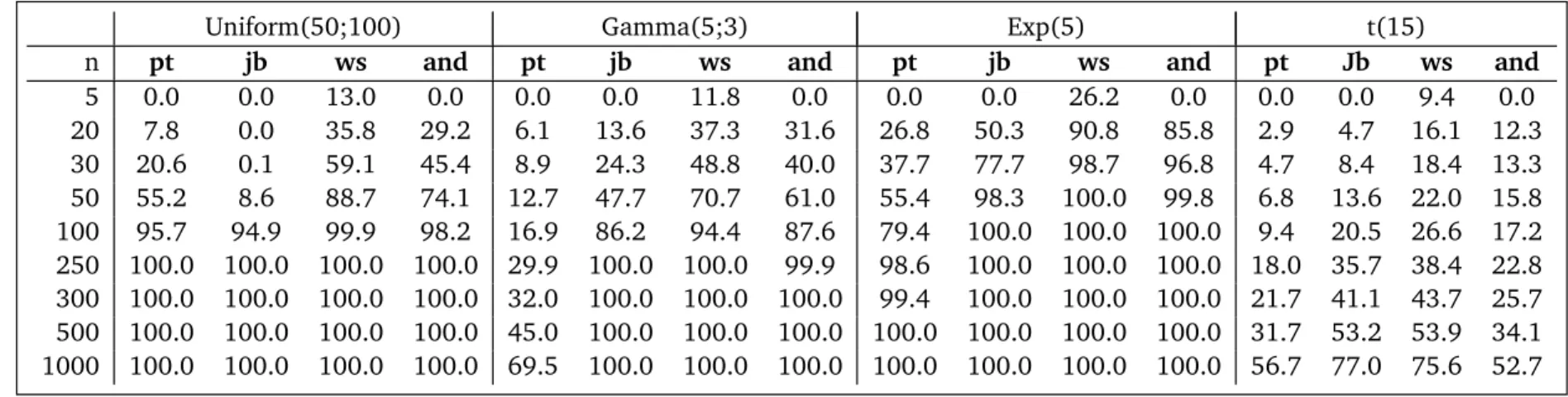
Secondly, in order to evaluate the power of the tests (and hence, Type II error rate), we gener-ated data from four other distributions: U ni f or m(50, 100),Gamma(5; 3), E x ponential(5), andS tud ent(15), using the same sample sizes. Results from the studies are reported in Ta-ble 1 and TaTa-ble 2. TaTa-ble 1 shows the Type I error percentages of: our proposed test (pt), Jarqua-Bera Test (jb), Shapiro-Wilk Test (ws), Anderson and Darling Test (and). These re-sults suggest our test is superior to the others. For almost all sample sizes evaluated, the false negative rate was much lower than the other tests. Even more interesting is the relative consistency demonstrated by our proposed test.

Table1: TypeIErrorProbabilitiesofComparedNormalityTests.

N(0; 1) N(50; 5)

n pt jb ws and pt jb ws and

5 0.0 0.0 9.8 0.0 0.0 0.0 9.4 0.0 20 1.1 2.0 12.5 10.1 1.6 2.1 12.3 10.0 30 1.7 3.4 12.3 10.3 1.8 3.7 12.4 10.0 50 2.0 4.7 12.0 10.0 1.8 4.4 12.4 10.5 100 1.9 6.0 12.3 10.3 2.0 6.1 12.1 9.9 250 1.9 7.6 11.2 10.0 2.0 7.6 12.0 10.1 300 1.7 7.9 12.0 10.2 1.8 7.6 11.5 9.3 500 2.1 9.1 12.2 9.7 1.8 8.2 11.4 9.8 1000 1.9 9.6 12.0 10.3 1.8 9.2 12.1 10.0

(6)

perfectly; much larger samples are required for the gamma distribution. Not surprisingly, when data were generated from the Student’s t distribution, none of the compared tests were sufficient to detect non-normality except for extremely large samples.

4. Concluding Remarks

In this study we proposed a novel normality test using the density function to transform data before testing. Of course, we have used very simple calculus methods. However, the simplicity of the calculus employed does not negate the value of our proposed test. Simulation studies show that the proposed test gives approximately perfect results for all sample sizes according to Type I error. However, according to Power, we can not say that our proposed test works better than the others. It is also seen that the Type I error rate seems invariant with respect to sample size, while the Type II error decreases with higher sample sizes. The logic underlying our test could be readily adapted to specific tests for other probability distributions. This could be a promising avenue of further research.

ACKNOWLEDGEMENTS The first author offers his thanks to The Scientific and Technolog-ical Research Council of Turkey (TUBITAK) for their support and encouragement of young Turkish researchers. The authors also thank the anonymous referee for assistance, which helped improve the presentation of this research.

References

[1] T Anderson and D Darling. A test of goodness of fit. Journal of the American Statistical Association, 49(268):765–769, 1954.

[2] C Jarque and A Bera. A test for normality of observation and regression residuals. Inter-national Statistical Review, 55(2):163–172, 1987.

(7)

F

E

R

E

N

C

E

S

4

5

4

Table2: PowerProbabilitiesofComparedNormalityTests.

Uniform(50;100) Gamma(5;3) Exp(5) t(15)

n pt jb ws and pt jb ws and pt jb ws and pt Jb ws and