Scientific Data Visualization with Shape Preserving C1 Rational Cubic Interpolation

Vol. 3, No. 2, 2010, 194-212

ISSN 1307-5543 – www.ejpam.com

Scientific Data Visualization with Shape Preserving

C

Rational

Cubic Interpolation

Malik Zawwar Hussain

_{, Muhammad Sarfraz}

_{, Maria Hussain}

2_{Department of Information Sciences, Adailiya Campus, Kuwait University, Kuwait} 3_{Lahore College for Women University, Lahore, Pakistan}

Abstract. This paper deals with the shape preserving C1_{rational cubic interpolation. The developed}

rational cubic interpolating function has only one free parameter. The approximation order of rational cubic function is investigated and range of optimal error constant is determined. Moreover, positive, constrained and monotone data preserving schemes are developed.

2000 Mathematics Subject Classifications: 68U05, 65D05, 65D07, 65D18.

Key Words and Phrases: Rational cubic, Spline, Peano Kernel theorem, Interpolation, Visualization.

1. Introduction

The development of interpolating and approximating techniques for shape control and shape preservation is a germane area of research in Computer Graphics and Data Visualization environment. The data are classified as positive, constrained, monotone and convex according to their shapes. Stability of radioactive substance and chemical reactions, solvability of solute in solvent, population statistics[3], resistance offered by an electric circuit, probability distri-bution[3]are a few examples of entities which are always positive. Monotonicity is applied in the specification of Digital to Analog Converters (DACs), Analog to Digital Converters (ADCs) and sensors. These devices are used in control system applications where non-monotonicity is unacceptable[9]. Erythrocyte sedimentation rate (E.S.R.) in cancer patients[9], uric acid level in patients suffering from gout[9], approximation of couples and quasi couples in statis-tics[2], data generated from stress of a material[9], rate of dissemination of drug in blood [2]are a few examples of entities which are always monotone.

∗_{Corresponding author.}

Email addresses:malikzawwarmath.pu.edu.pk(M. Z. Hussain),prof.m.sarfrazgmail.om(M.

Sarfraz),mariahussain_1yahoo.om(M. Hussain)

In the past quite a few authors have worked in the area of shape preserving interpolation. The positivity preserving scheme, by Butt and Brodlie [3], preserved the shape of data by interval subdivision technique. In the interval, where the piecewise cubic interpolant lost the positive shape of data, the authors inserted an additional knot (increase in number of data points) in such a way that original shape of the data was preserved. Fahr and Kallay[5]used a monotone rational B-spline of degree one to preserve the shape of monotone data. Goodman et al[7]developed rational cubic interpolating schemes to preserve the shape of data lying on the either side of straight line. The first scheme scaled weights by some scale factors and the second scheme adopted the method of insertion of a new interpolation point. Goodman [8]surveyed the shape preserving interpolating schemes for planar data. Hussain and Sarfraz used four parameter family of rational cubic function to preserve the shape of positive and monotone data in[10]and[11]respectively. Lamberti and Manni[12]used cubic Hermite in parametric form to preserve the shape of data. The step length was used as shape preserving parameters. The first order derivatives at the knots were estimated imposing second derivative continuity at the knots, which resulted in tridiagonal system of equations. Sarfraz et al[13] addressed the problems of positive and monotone curve data interpolation using rational cubic function with two parameters. Sarfraz et al [14]developed aGC1 cubic function with one free parameter to preserve the positive, monotone and convex data. Schmidt and Hess[15] developed sufficient conditions on derivatives at the knots to assure positivity of interpolating cubic polynomial.

This paper presents shape preserving interpolating schemes for positive, constrained and monotone data. A one parameter family of rational cubic function has been developed to pre-serve the shape of the data. In different intervals, the free parameter adopts different value. That is, the interpolant has same structure but different functions in different intervals. The presented schemes are neither dependent on data nor on derivatives. Unlike the methodolo-gies in[3, 7,12], the scheme developed in this paper does not constrain interval length. The developed scheme is equally applicable whether the data is with derivatives or the derivative is estimated by derivative estimation techniques[10-11]. The schemes presented in this paper use one parameter family of rational function to preserve the shape of data thus computation-ally less expansive than[10-11, 13]. The order of continuity achieved isC1, whereas, in[14] it wasGC1.

The remainder of the paper is organized as follows. In Section 2, the C1 rational cubic interpolant with one free parameter is developed and Section 2.1 discusses its approximation properties. The visualization problems of positive, constrained, and monotone data interpo-lation are discussed in Sections 3, 4 and 5 respectively. Section 6 concludes the paper.

2. Rational Cubic Function

In this Section, a C1 rational cubic function with one parameter and linear denominator has been developed. Let{(x_i,f_i), i=0, 1, 2, . . . ,n}be a given set of data points defined over the interval [a,b], where a = x0 < x1 < x2 < · · · < xn = b. The C1 piecewise rational

0, 1, 2, . . . ,n−1 as:

S(x)≡Si(x) =

p_i(θ)

q_i(θ), (1)

where

pi(θ) = 3

X

i=0

(1−θ)3−iθAi,

A₀ = (α_i+1)f_i,

A₁ = (2α_i+3)f_i+h_id_i, A2 = (αi+3)fi+1−hidi+1,

A3 = fi+1,

q_i(θ) = 1+α_i(1−θ),

h_i = x_i+1−x_i, θ = (x−xi)

h_i ,

S(x_i) = f_i, S(x_i+1) = f_i+1, S(1)(x_i) =d_i, S(1)(x_i+1) =d_i+1. (2) S(1)(x)denotes the derivative with respect toxanddi denotes derivative values estimated or

given. It is noted that whenα_i=0, the piecewise rational cubic function (1) reduces to cubic Hermite spline. In this paper, the parameterα_i can assume any positive real value.

2.1. Error Estimation of Interpolation

In this Section, the error of interpolation is estimated when the function being interpolated is f(x)∈C2[x₀,x_n]. The interpolation scheme developed in Section 2 is local, which allows investigating the error in an arbitrary subinterval Ii = [xi,xi+1] without loss of generality.

Using Peano Kernel Theorem[16]the error of interpolation in each subintervalI_i= [x_i,x_i+1]

is:

R[f] = f(x)−Si(x) =

1 2

Z xi+1

xi

f(2)(τ)Rx[(x−τ)+]dτ. (3)

It is assumed that the function being interpolated is f(x)∈C2[x₀,x_n]. The absolute error in Ii = [xi,xi+1]is:

|f(x)−S_i(x)| ≤ 1

2kf

(2)_(τ)k

Z xi+1

xi

|R_x[(x−τ)₊]|dτ, (4)

where

R_x[(x−τ)₊] =

¨

u(τ,x), xi< τ <x,

v(τ,x), x< τ <x_i+1.

«

, (5)

The integral involved in (4) is expressed as:

Z xi+1

xi

|Rx[(x−τ)+]|dτ=

Z x

xi

|u(τ,x)|dτ+

Z xi+1

x

For theC1rational cubic function (1),u(τ,x)andv(τ,x)have the values

u(τ,x) = (x−τ)− θ 2

q_i(θ)[(1−θ){(αi+3)(xi+1−τ)−hi}+θ(xi+1−τ)], (7)

v(τ,x) = − θ 2

q_i(θ)[(1−θ){(αi+3)(xi+1−τ)−hi}+θ(xi+1−τ)]. (8)

The roots ofu(x,x)andv(x,x)in[0, 1]areθ=0 andθ=1. The root ofu(τ,x) =0 isτ₁= x− hiθ2(αi+2)

(αi+1)+θ(αi+2).

The root of v(τ,x) =0 isτ2= xi+1−

hi(1−θ)

1+(αi+2)(1−θ).

The above discussion leads to the following manipulation:

|f(x)−S_i(x)| ≤ 1

2kf

(2)_(τ)kh2

iω(αi,θ), ω(α_i,θ) =

Z x

xi

|u(τ,x)|dτ+

Z xi+1

x

|v(τ,x)|dτ

=

Z τ1

xi

u(τ,x)dτ−

Z x

τ1

u(τ,x)dτ−

Z τ2

x

v(τ,x)dτ+

Z xi+1

τ2

v(τ,x)dτ

= θ

2_{−θ2_(α

i+2)2qi(θ) + (αi+1)2(1+θ)2((αi+3)−θ(αi+2))}

q_i(θ){1+α_i+θ(α_i+2)}2

+2θ

2_(1−θ)2

q_i(θ) −

2θ4(1−θ)(α_i+2)

q_i(θ){1+α_i+θ(α_i+2)}+

θ2(1−θ)2

q_i(θ){1+ (α_i+2)(1−θ)}.

The above discussion is summarized as follows:

Theorem 1. The error of C1 rational cubic function (1), for f(x)∈C2[x₀,x_n], in each subin-terval I_i= [x_i,x_i+1]is

|f(x)−S_i(x)| ≤1

2kf

(2)_(τ)kh2

ici, (9)

where c_i is the maximum value ofω(α_i,θ)for0≤θ ≤1andα_i≥0.

Theorem 2. For any given positive parameterα_i, the error optimal constant c_i in Theorem 1 are bounded with0≤c_i≤0.2685.

3. Positivity Preserving Interpolation

This section provides sufficient conditions on parameters for positive interpolation of curve data. Let{(xi,fi), i=0, 1, 2, . . . ,n}be the positive data defined over the interval[a,b]. The

necessary condition for the positivity of data is

The piecewise rational cubic function (1) preserves positivity if Si(x)>0, i=0, 1, 2, . . . ,n−1.

Now,S_i(x)>0 if

pi(θ)>0 and qi(θ).

But,qi(θ)if

α_i >0.

Using the result developed by Schmidt and Hess in[15], the cubic polynomialp_i(θ)>0 if

(p′_i(0),p_i′(1))∈R₁UR₂, where

R₁ =

(a, b):a> −3fi

hi

, b< 3fi+1

hi

,

R₂ = {(a,b): 36f_if_i+1(a2+b2+a b−3∆i(a+b) +3∆2i) +4hi(a3fi+1−b3fi)

+3(a fi+1−b fi)(2hia b−3a fi+1+3b fi)−h2ia

2_b2_≥0}.

For the rational cubic function (1), we have

p′_i(0) = −αifi+hidi

hi

andp′_i(1) =−αifi+1+hidi+1

hi

.

(p′_i(0), p′_i(1))∈R₁ if

−αifi+hidi

hi

> −3fi

hi

, (11)

and

−α_if_i+1+hidi+1

h_i < 3f_i+1

h_i . (12)

The inequality (11) leads to the following relation:

α_i< hidi

fi

+3. (13)

The inequality (12) imposes the following restriction on the free parameterα_i:

α_i > hidi+1

f_i+1

−3. (14)

Further(p′_i(0), p′_i(1))∈R₂if

φ(αi) = 36fifi+1[φ12(αi) +φ22(αi) +φ1(αi)φ2(αi)−3∆i(φ1(αi) +φ2(αi)) +3∆2i]

+3[fi+1φ1(αi)−fiφ2(αi)][2hiφ1(αi)φ2(αi)−3fi+1φ1(αi) +3fiφ2(αi)]

Theorem 3. The piecewise C1 rational cubic interpolant S(x), defined over the interval[a,b], in (1), is positive if in each subinterval I_i = [x_i,x_i+1] the following sufficient conditions are satisfied:

C on₁< α_i<C on₂, where

C on1=M a x

0,hidi+1 f_i+1 −3

and C on2=

h_id_i f_i +3. The above constraints can be rearranged as:

C on1+ki=αi =C on2−li,

where k_i>0and l_i>0.

Thus we have the following algorithm for the manipulation of positive curve design.

Algorithm 1

Step 1. Enter the(n+1)positive data points{(x_i,f_i): i=0, 1, 2, . . . ,n}.

Step 2. Estimate the first order derivatives d_i, i =0, 1, 2, . . . ,nat knots. (Note: The step 2 is only applicable if data is not provided with derivatives).

Step 3. Calculate the value of free parameterα_i using Theorem 3.

Step 4. Substitute the values of fi, di, i= 0, 1, 2, . . . ,nandαi, i=0, 1, 2, . . . ,n−1 in

rational cubic function (1) to obtain positive curve through positive data.

3.1. Demonstration

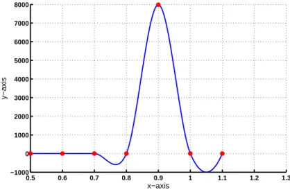
Example 1. A positive data set in Table 1 is taken from [6]. The Figure 1 is produced from

Table1: Apositivedata takenfrom[6℄.

x 0.5 0.6 0.7 0.8 0.9 1.0 1.1

f 0.4804 0.5669 0.7262 0.1 7985 0.8658 0.9281

the data set in Table 1 using the cubic Hermite spline interpolation technique which loses the positive shape of data. The positive curve in Figure 2 is produced by using positive curve data interpolation scheme developed in Section 3.

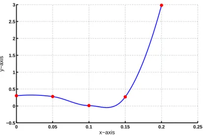
Example 2. The positive data set in Table 2 is taken from[6]. The Figure 3 is produced from the

Table2: Anotherpositivedatatakenfrom[6℄.

0.5 0.6 0.7 0.8 0.9 1 1.1 1.2 1.3 −1000

0 1000 2000 3000 4000 5000 6000 7000 8000

x−axis

y−axis

Figure1: CubiHermitespline.

0.5 0.6 0.7 0.8 0.9 1 1.1 1.2 1.3

0 1000 2000 3000 4000 5000 6000 7000 8000

x−axis

y−axis

Figure2: PositiveC

1

0 0.05 0.1 0.15 0.2 0.25 −0.5

0 0.5 1 1.5 2 2.5 3

x−axis

y−axis

Figure3: CubiHermitespline.

0 0.05 0.1 0.15 0.2 0.25

0 0.5 1 1.5 2 2.5 3

x−axis

y−axis

Figure4: PositiveC

1

4. Constrained Data Interpolation

Let{(x_i, f_i), i=0, 1, 2, . . . ,n}be the given set of data points lying above the straight line y=mx+c i.e.

f_i>mx_i+c, ∀ i=0, 1, 2, . . . ,n. (16) The curve will lie above the straight line if the C1 rational cubic function (1) satisfies the following condition:

S(x)>mx+c, ∀x∈[x0,xn].

For each subintervalI_i= [x_i,x_i+1], the above relation in parametric form is expressed as

S_i(x)>a_i(1−θ) +b_iθ, (17) whereθ= x−xi

hi andai(1−θ)+biθis the parametric equation of straight line withai =mxi+c

andb_i=mx_i+1+c. The rearrangement of (17) leads to the following relation:

U_i(θ) = 3

X

i=0

(1−θ)3−iθiB_i, (18)

where

B₀ = (α_i+1)(f_i−a_i),

B₁ = α_i(2f_i−a_i−b_i) +3f_i−2a_i−b_i+h_id_i, B₂ = (α_i+2)(f_i+1−b_i) +f_i+1−h_id_i+1−a_i, B₃ = f_i+1−bi.

Now, U_i(θ)>0 ifB_i >0,i=0, 1, 2, 3. It is straightforward to know thatB₀ >0 and B₃ >0 are true from the necessary condition defined in (16) andα_i>0.B₁>0 provides the follow-ing constraints onαi:

If 2f_i−a_i−b_i>0 thenα_i >−fi+bi−hidi

2fi−ai−bi . Similarly, if 2fi−ai−bi<0 thenαi<

−fi+bi−hidi

2fi−ai−bi .

One can also note thatB₂>0 ifα_i> −fi+1+hidi+1+ai fi+1−bi .

The above discussion can be summarized as:

Theorem 4. The piecewise C1 rational cubic interpolant S(x), defined over the interval[a, b], in (1), preserves the shape of data that lies above the straight line if in each subinterval I_i = [x_i,x_i+1]the following sufficient conditions are satisfied:

C on₃ < α_i <C on₄, C on₃ = M a x

0,−fi+bi−hidi 2f_i−a_i−b_i ,

−f_i+1+h_id_i+1+a_i

f_i+1−b_i

,

C on4 =

−f_i+b_i−h_id_i

The above constraints can be rearranged as:

C on3+mi=αi=C on4−ni,

where m_i >0and n_i>0.

Thus we have the following algorithm for the manipulation of curve design.

Algorithm 2

Step 1. Enter the(n+1)positive data points{(x_i,f_i): i=0, 1, 2, . . . ,n}.

Step 2. Estimate the first order derivatives di, i =0, 1, 2, . . . ,nat knots. (Note: The

step 2 is only applicable if data is not provided with derivatives). Step 3. Calculate the value of free parameterα_iusing Theorem 4.

Step 4. Substitute the values of fi, di, i= 0, 1, 2, . . . ,nandαi, i=0, 1, 2, . . . ,n−1 in

rational cubic function (1) to obtain the curve lying above the straight line.

4.1. Demonstration

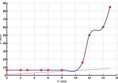
Example 3. The data set in Table 3 is lying above the straight line y = ₂x +1and is taken from [1]with slight modification. The Figure 5 is produced from the data set in Table 3 using cubic

Table3:

x 0 2 3 5 6 8 11 12 14 15

f 6.5 6.5 6.5 6.5 6.5 6.5 16 50 60 85

Hermite spline. It is clear from the Figure 5 that some part of the curve is lying below the line y = x

2 +1. This flaw is recovered nicely in Figure 6 using constrained data interpolation scheme

developed in Section 4. It is clear from Figure 6 shape of the data is recovered.

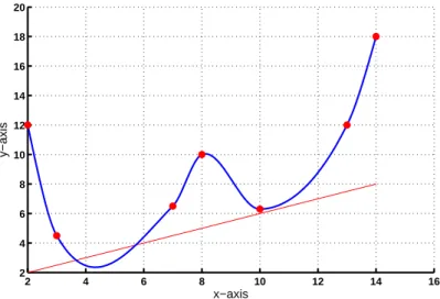
Example 4. The data set[10]in Table 4 is lying above the straight line y = x

2 +1. Figure 7

Table4: Thedatasetlyingabove thestraightline y=

x 2+1.

x 2 3 7 8 10 13 14

f 12 4.5 6.5 10 6.3 12 18

is produced from the data set in Table 4 using cubic Hermite spline. It is clear from Figure 7 that cubic Hermite spline loses the shape of data. Figure 8 is produced from the same data set using constrained curve data interpolation scheme developed in Section 4. It is clear from the Figure 8 that curve is lying above the straight line y= x

0 2 4 6 8 10 12 14 16 0

10 20 30 40 50 60 70 80 90

x−axis

y−axis

Figure5: CubiHermitespline.

0 2 4 6 8 10 12 14 16

0 10 20 30 40 50 60 70 80 90

x−axis

y−axis

Figure6: ConstrainedC

1

2 4 6 8 10 12 14 16 2

4 6 8 10 12 14 16 18 20

x−axis

y−axis

Figure7: CubiHermitespline.

2 4 6 8 10 12 14 16

2 4 6 8 10 12 14 16 18 20

x−axis

y−axis

Figure8: ConstrainedC

1

5. Monotonicity Preserving Interpolation

Let{(x_i,f_i), i=0, 1, 2, . . . ,n}be the monotone data defined over the interval[a,b]such that

∆_i = fi+1− fi

hi

>, d_i>0, i=0, 1, 2, . . . ,n−1. (19)

The piecewise rational cubic function (1) preserves monotonicity if S(1)(x)>0, i=0, 1, 2, . . . ,n−1, where

S_i(1)(x) =

P3

i=0(1−θ) 3−i_θi_C

i

(qi(θ))2

, (20)

C0 = (αi+1)di,

C1 = (αi+1){(2αi+6)∆i−2di+1−di},

C₂ = (4α_i+6)∆_i−d_i+1−2d_i, C₃ = d_i+1.

From (20),S_i(1)(x)if C_i >0, i=0, 1, 2, 3. We know thatC₀ >0 and C₃ >0 are always true from the necessary condition of monotonicity defined in (19) andαi >0. One can see that

C₁>0 if

α_i>M a x

0,2di+1+di 2∆_i

.

Similarly,C₂>0 if

α_i>M a x

0,di+1+2di 4∆_i

.

The above can be summarized as:

Theorem 5. The piecewise C1 rational cubic interpolant S(x), defined over the interval[a,b], in (1), is monotone if in each subinterval I_i = [x_i,x_i+1]the following sufficient conditions are satisfied:

α_i>M a x

0,2di+1+di 2∆_i ,

d_i+1+2d_i 4∆_i

.

The above constraints can be rearranged as:

α_i =m_i+M a x

0,2di+1+di 2∆_i ,

d_i+1+2di

4∆_i

, m_i>0.

Algorithm 3

Step 1. Enter the(n+1)points{(x_i, f_i): i=0, 1, 2, . . . ,n}.

Step 2. Estimate the first order derivatives d_i, i=0, 1, 2, . . . ,nat knots. (Note: The step 2 is only applicable if data is not provided with derivatives).

Step 3. Calculate the value of free parameterα_i using Theorem 5. Step 4.

If∆_i>0 then d_i=0

S(x)≡Si(x) = fi

else

S(x)≡Si(x) = pi(θ) qi(θ)

end

5.1. Demonstration

Table5: Amonotonedataset.

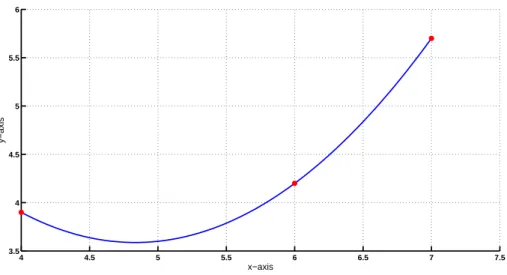
x 4.0 6.0 7.0 f 3.9 4.2 5.7

Example 5. A monotone data set is taken in Table 5. Non-monotone curve in Figure 9 is produced from the monotone data set taken in Table 5 using cubic Hermite spline. The monotone curve (from the same data set) is produced in Figure 10 using monotonicity preserving scheme developed in Section 5.

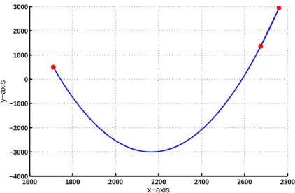
Table6: Amonotonedataset.

x 1710 2650 2760 f 500 1360 2940

4 4.5 5 5.5 6 6.5 7 7.5 3.5

4 4.5 5 5.5 6

x−axis

y−axis

Figure9: CubiHermitespline.

4 4.5 5 5.5 6 6.5 7 7.5

3.5 4 4.5 5 5.5 6

x−axis

y−axis

Figure10: MonotoneC

1

1600 1800 2000 2200 2400 2600 2800 −4000

−3000 −2000 −1000 0 1000 2000 3000

x−axis

y−axis

Figure11: CubiHermitespline.

1600 1800 2000 2200 2400 2600 2800

500 1000 1500 2000 2500 3000

x−axis

y−axis

Figure12: MonotoneC

1

6. Conclusion

The work in this paper is concerned to the development of shape preserving interpolating schemes. The developed schemes have the following advantageous features over the existing schemes. These are equally worthy for data with and without derivatives, whereas, authors in [15] had to constrain derivatives at knots to preserve the shape of positive data. The developed schemers are based on automated selection of free parameters thus do not require the modification of data. But, the authors in [3, 7, 12] constrained the interval length to preserve the shape of data. In[13]and[10-11], rational functions with two and four family of free parameters were used to preserve the shape of data hence computationally expansive than shape preserving schemes developed in this paper. The order of continuity attained in [14]wasGC1, whereas, in this paper it isC1.

References

[1] Akima, H., A new method of interpolation and smooth curve fitting based on local procedures,Journal of the Association for Computing Machinery,17, (1970), 589-602. [2] Beliakov, G., Monotonicity preserving approximation of multivariate scattered data,BIT,

45(4), (2005), 653-677.

[3] Butt, S. and Brodlie, K. W., Preserving positivity using piecewise cubic interpolation, Computers and Graphics,17(1), (1993), 55-64.

[4] Duan, Q., Zhang, H., Zhang, Y. and Twizell, E. H., Error estimation of a kind of rational spline,Journal of Computational and Applied Mathematics,200(1), (2007), 1-11. [5] Fahr, R. D. and Kallay, M., Monotone linear rational spline interpolation,Computer Aided

Geometric Design,9, (1992), 313-319.

[6] Gerald, C. F. and Wheatley, P. O., Applied Numerical Analysis, 7th Edition, Addison Wesley Publishing Company, (2003).

[7] Goodman, T. N. T., Ong, B. H. and Unsworth, K., Constrained interpolation using ratio-nal cubic splines, Proceedings of NURBS for Curve and Surface Design, G. Farin (eds), (1991), 59-74.

[8] Goodman, T. N. T., Shape preserving interpolation by curves, Proceeding of Algorithms for Approximation IV, J. Levesley, I. J. Anderson and J. C. Mason(eds.), University of Huddersfeld, (2002), 24-35.

[9] Hussain, M. Z. and Hussain, M., Visualization of data preserving monotonicity,Applied Mathematics and Computation,190, (2007), 1353-1364.

[11] Hussain, M. Z. and Sarfraz, M., Monotone piecewise rational cubic interpolation, To be appeared inInternational Journal of Computer Mathematics,86, (2009).

[12] Lamberti, P. and Manni, C., Shape-preserving functional interpolation via parametric cubics,Numerical Algorithms,28, (2001), 229-254.

[13] Sarfraz, M., Butt, S. and Hussain, M. Z., Visualization of shaped data by a rational cubic spline interpolation,Computers and Graphics,25(5), (2001), 833-845.

[14] Sarfraz, M., Hussain, M. Z. and Chaudhry, F. S., Shape preserving cubic spline for data visualization,Computer Graphics and CAD/CAM,01, (2005), 189-193.

[15] Schmidt, J. W. and Hess, W., Positivity of cubic polynomial on intervals and positive spline interpolation,BIT,28, (1988), 340-352.