Efficient Pre-Processing for Large Window-Based Modular Exponentiation
Using Ant Colony
Nadia Nedjah
Department of Electronics Engineering and Telecommunications, Faculty of Engineering, State University of Rio de Janeiro, Brazil [email protected]
Luiza de Macedo Mourelle
Department of Systems Engineering and Computation,
Faculty of Engineering, State University of Rio de Janeiro, Brazil [email protected]
Keywords:ant colony, addition chain, cryptosystem, modular exponentiation Received:September 30, 2004
Modular exponentiation is the main operation to RSA-based public-key cryptosystems. It is performed using successive modular multiplications. This operation is time consuming for large operands, which is always the case in cryptography. For software or hardware fast cryptosystems, one needs thus reducing the total number of modular multiplications required. Existing methods attempt to reduce this number by partitioning the exponent in constant or variable size windows. However, these window-based methods require some computations, which themselves consist of modular exponentiations. It is clear that pre-processing needs to be performed efficiently also. In this paper, we exploit the ant colony strategy to finding an optimal addition sequence that allows one to perform the pre-computations in window-based methods with a minimal number of modular multiplications. Hence we improve the efficiency of modular exponentiation. We compare the yielded addition sequences with those obtained using Brun’s algorithm. Povzetek: Metoda kolonij mravelj je uporabljena za kriptografske probleme.
1 Introduction
Public-key cryptographic systems (such as the RSA en-cryption scheme [6], [12]) often involve raising large el-ements of some groups fields (such as GF(2n) or elliptic
curves [9]) to large powers. The performance and practi-cality of such cryptosystems is primarily determined by the implementation efficiency of the modular exponentiation. As the operands (the plain text of a message or the cipher (possibly a partially ciphered) are usually large (i.e. 1024 bits or more), and in order to improve time requirements of the encryption/decryption operations, it is essential to at-tempt to minimise the number of modular multiplications performed.
A simple procedure to computeC=TEmodM based
on the paper-and-pencil method is described in Algorithm 1. This method requires E-1 modular multiplications. It computes all powers of T: T → T2 → . . . → TE−1 →TE.
Algorithm 1.simpleExponentiation(T, M, E)
1. C:=T;
2. fori:= 1toE−1doC:= (C×T)modM; 3. returnC;
end algorithm.
The computation of exponentiations using Algorithm 1 is very inefficient. The problem of yielding the power of a number using a minimal number of multiplications isN P -hard [5], [10]. There are several efficient algorithms that perform exponentiation with a nearly minimal number of modular multiplications, such that the window-based meth-ods. However, these methods need some pre-computations that if not performed efficiently can deteriorate the al-gorithm overall performance. The pre-computations are themselves an ensemble of exponentiations and so it is also
N P-hard to perform them optimally. In this paper, we con-centrate on this problem and engineer a new way to do the necessary pre-computations very efficiently. We do so us-ing the ant colony methodology. We compare our results with those obtained using the Brun’s algorithm [1].
ca-pable to return quicker and so the pheromone deposited on that path increases relatively faster than that deposited on much longer alternative paths. Consequently, all the ants of the colony end using the shorter way.
In this paper, we exploit the ant colony methodology to obtain an optimal solution to AS-chain minimisationNP -complete problem. In order to clearly report the research work performed, we subdivide the rest of this paper into five important sections. In Section 2, we present the win-dow methods; In Section 3, we present the concepts of ad-dition chains and sequence and they can be used to improve the pre-computations of the window methods; In Section 4, we give an overview on ant colony concepts; In Section 5, we explain how these concepts can be used to compute a minimal addition chain to perform efficiently necessary pre-computations in the window methods. In Section 6, we present some useful results.
2 Window-Based Methods
Generally speaking, the window methods for exponentia-tion [5] may be thought of as a three major step procedure: 1. partitioning ink-bits windows the binary
representa-tion of the exponentE;
2. pre-computing the powers in each window one by one; 3. iterating the squaring of the partial resultk times to shift it over, and then multiplying it by the power in the next window when if window is not 0.
There are several partitioning strategies. The window size may be constant or variable. For the m-ary methods, the window size is constant and the windows are next to each other. On the other hand, for the sliding window meth-ods the window size may be of variable length. It is clear that zero-windows, i.e. those that contain only zeros, do not introduce any extra computation. So a good strategy for the sliding window methods is one that attempts to max-imise the number of zero-windows. The details ofm-ary methods are exposed in Section 2.1 while those related to sliding constant-size window methods are given in Section 2.2. In Section 2.3, we introduce the adaptive variable-size window methods.
2.1
M
-ary Methods
Them-ary methods [3] scans the digits of E form the less significant to the most significant digit and groups them into partitions of equal lengthlog2m, wheremis a power of two. Note that 1-ary methods coincides with the square-and- multiply well-known binary exponentiation method.
In general, the exponent E is partitioned intop parti-tions, each one containing l = log2m successive digits. The ordered set of the partition of E will be denoted by
P(E). If the last partition has less digits thanlog2m, then the exponent is expanded to the left with at mostlog2m−1
zeros. The m-ary algorithm is described in Algorithm 2, whereinVidenotes the decimal value of partitionPi.
Algorithm 2.m-aryMethod(T, M, E)
1. PartitionEintop l-digits partitions; 2. fori:= 2tomComputeTimodM;
3. C:=TVpmodM; 4. fori:=p−2downto 0 5. C:=C2lmodM;
6. ifVi6= 0thenC:=C×modM;
7. returnC; end algorithm.
2.2 Sliding Window Methods
For the sliding window methods the window size may be of variable length and hence the partitioning may be performed so that the number of zero-windows is as large as possible, thus reducing the number of modular multiplication necessary in the squaring and multiplication phases. Furthermore, as all possible partitions have to start (i.e. in the right side) with digit 1, the pre-processing step needs to be performed for odd values only. The sliding method algorithm is presented in Algorithm 3, wherein d denotes the number of digits in the largest possible partition andLithe length of partitionPi.
Algorithm 3.slidingWindowMethod(T, M, E)
1. PartitionEusing the given strategy; 2. fori:= 2to2d−1step 2 do
3. ComputeTimodM;
4. C:=TVp−1modM; 5. fori:=p−2downto 0 do 6. C:=CLimodM;
7. ifVi6= 0thenC:=C×TVimodM;
8. returnC; end algorithm.
In adaptive methods [7] the computation depends on the input data, such as the exponent E. M-ary methods and window methods pre-compute powers of all possible parti-tions, not taking into account that the partitions of the ac-tual exponent may or may not include all possible parti-tions. Thus, the number of modular multiplications in the pre-processing step can be reduced if partitions of E do not contain all possible ones.
Let℘(E)be the list of partitions obtained from the bi-nary representation ofE. Assume that the list of partition is non-redundant and ordered according to the ascending decimal value of the partitions contained in the expansion ofE. Recall thatViandLiare the decimal value and the
number of digits of partitionPi. The generic algorithm for
describing the computation ofTE modM using the
win-dow methods is given in Algorithm 4.
step of the 4-ary method needs 14 modular multiplica-tions (T → T ×T = T2 → T ×T2 = T3 → →
T ×T14 =T15)and that of the maximum 4-digit sliding window method needs only 8 modular multiplications
(T → T ×T = T2 → T ×T2 = T3 → T3×T2 =
T5 → T5 ×T2 = T7 → → T13 ×T2 = T15). However the adaptive 4-ary method would partition the exponent as E = 1011k0011k0111k1000 and hence needs to pre-compute the powers T3, T7, T8 and T11 while the method maximum 4-digit slid-ing window method would partition the exponent as
E = 1k0k11k00k11k0k1111k000and therefore needs to pre-compute the powersT3andT15. The pre-computation of the powers needed by the adaptive 4-digit sliding win-dow method may be done using 6 modular multiplications
T →T×T =T2→T×T2=T3→T2×T2=T4→
T3×T4 = T7 → T7×T = T8 → T8×T3 = T11 while the pre-computation of those powers neces-sary to apply the adaptive sliding window may be accomplished using 5 modular multiplications
T →T×T =T2→T×T2=T3→T2×T3=T5→
T5×T5=T10→T5×T10=T15. Note that Algorithm 4 does not suggest how to compute the powers (lines 2–3) needed to use the adaptive window methods. Finding the best way to compute them is aN P-hard problem [4], [7].
Algorithm 4.AdaptiveWindowMethod(T, M, E)
1. PartitionEusing the given strategy; 2. for each partitionPi∈℘do
3. ComputeTVimodM; 4. C:=TVp−1modM; 5. fori:=p−2downto 0 do 6. C:=CLimodM;
7. ifVi6= 0thenC:=C×TVimodM;
8. returnC; end algorithm.
3 Addition Chains and Sequences
Anaddition chainof lengthlfor an positive integerN is a list of positive integers(E1, E2, . . . , El)such thatE1= 1,
El=NandEk =Ei+Ej,0 ≤i≤j < k ≤l. Finding
a minimal addition chain for a given positive integer is an
N P-hard problem. It is clear that a short addition chain for exponentEgives a fast algorithm to computeTEmod
M as we have ifEk =Ei+Ej thenTEk =TEi×TEj.
The adaptive window methods described earlier use a near optimal addition chain to computeTE modM. However
these methods do not prescribe how to perform the pre-processing step (Line 3 of Algorithm 4). In the following we show how to perform this step with minimal number of modular multiplications.
3.1 Addition sequences
There is a generalisation of the concept of addition chains, which can be used to formalise the problem of finding a minimal sequence of powers that should be computed in the pre-processing step of the adaptive window method.
An addition sequence for the list of positive integers
V1, V2,. . .,Vp such thatV1 < V2 < . . . < Vp is an
ad-dition chain for integer Vp that includes all the integers
V1, V2, . . . , Vp. The length of an addition sequence is the
numbers of integers that constitute the chain. An addition sequence for a list of positive integersV1, V2, . . . , Vp will
be denoted byξ(V1, V2, . . . , Vp).
Hence, to optimise the number of modular required mul-tiplications in the pre-processing step of the adaptive win-dow methods for computingTEmodM, we need to find
an addition sequence of minimal length (or simply minimal addition sequence) for the values of the partitions included in the non-redundant ordered list ℘(E). This is an N P -hard problem and we use genetic algorithm to solve it. Our method showed to be very effective for large window size. General principles of genetic algorithms are explained in the next section.
3.2 Brun’s algorithm
Now we describe briefly, Brun’s algorithm [1] to compute addition sequences. The algorithm is a generalisation of the continued fraction algorithm [1]. Assume that we need to compute the addition sequence ξ(V1, V2, . . . , Vp). Let
Q=b Vp
Vp−1cand letχ(Q)be the addition chain forQ us-ing the binary method (i.e. that used in Algorithm 2 withl= 1). LetR=Vp−Q×Vp−1. By induction we can construct
an addition sequenceξ(V1, V2, . . . , R, . . . , Vp−1), then ob-tain:
ξ(S) = ξ(V1, V2, . . . , R, . . . , Vp−1)∪
Vp−1×χ(Q)\ {1} ∪ {Vp},
S = V1, V2, . . . , Vp
(1)
4 Ant Systems and Algorithms
Ant systems can be viewed as multi-agent systems [3] that use a shared memory through which they communicate and a local memory to bookkeep the locally reached problem solution. Fig. 1. depicts the overall structure of an system, whereinAiandLMirepresent theith.agent of the ant
sys-tem and its local memory respectively. Mainly, the shared memory (SM) holds the pheromone information while the local memory LMi keeps the solution (possibly partial)
that agentAireached so far.
Figure 1: Multi-agent system architecture
The first step consists of activating N distinct artificial ants that should work in simultaneously. Every time an ant conclude its search, the shared memory is updated with an amount of pheromone, which should be proportional to the quality of the reached solution. This called global
pheromone update. When the solution yield by an ant’s work is suitable (i.e. fits characteristics C) then all the active ants are stopped. Otherwise, the process is iterated until an adequate solution is encountered.
Algorithm 5.ArtificialAntColony(N, C)
1. InitialiseSMwith initial pheromone; 2. do
3. fori:= 1toN
4. Start ArtificialAnt(Ai, LMi);
5. Active:=Active∪ {Ai};
6. do
7. UpdateSM(pheromone evaporation); 8. when an ant (sayAi) halts do
9. Active:=Active\ {Ai};
10. Φ:= Pheromone(LMi);
11. UpdateSM(global pheromoneΦ); 12. S:= ExtractSolution(LMi);
13. until Fitness(S) =CorActive=∅; 14. whileActive6=∅do
15. Stop antAi|Ai∈Active;
16. Active:=Active\ {Ai};
17. until Fitness(S) =C; 18. returnS;
end.
The behaviour of an artificial ant is described in Algorithm 6, wherein Ai and LMi represent the ant
identifier and the ant local memory, in which it stores the solution computed so far. First, the ant computes the probabilities that it uses to select the next state to move to. The computation depends on the solution built so far, the problem constraints as well as some heuristics [2], [6].
Thereafter, the ant updates the solution stored in its local memory, deposits some localpheromone into the shared memory then moves to the chosen state. This process is iterated until complete problem solution is yielded.
Algorithm 6.ArtificialAnt(Ai, LMi)
1. InitialiseLMi;
2. do
3. P := TransitionProbabilities(LMi);
4. N extState:= StateDecision(LMi, P);
5. UpdateLMi;
6. UpdateSMwith local pheromone; 7. CurrentState:=N extState); 8. untilCurrentState:=T argetState; 9. HaltAi;
end.
5 Chain Sequence Minimisation
Using Ant System
In this section, we concentrate on the specialisation of the ant system of Algorithm 4 and Algorithm 5 to the addi-tion sequence minimisaaddi-tion problem. For this purpose, we describe how the shared and local memories are repre-sented. We then detail the function that yields the solution (possibly partial) characteristics. Thereafter, we define the amount of pheromone to be deposited with respect to the solution obtained so far. Finally, we show how to compute the necessary probabilities and make the adequate decision towards a shorter addition sequence for the considered the sequence(V1, V2, . . . , Vp).
5.1 The Ant System Shared Memory
The ant system shared memory is a two-dimension array. If the last exponent in the sequence is Vp then the array
shouldVp rows. The number of columns depends on the
row. It can be computed as in Eq. 2, whereinN Cidenotes
the number of columns in rowi.
N Ci=
2i−1−i+ 1 if2i−1< V
p
1 ifi=Vp
Vp−i+ 3 otherwise
(2)
An entrySMi,jof the shared memory holds the pheromone
deposited by ants that used exponenti+jas theith. mem-ber in the built addition sequence. Note that1 ≤ i ≤Vp
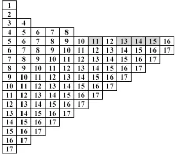
and for row i,0 ≤ j ≤ N Ci. Fig. 2 gives an example
of the shared memory for exponent 17. In this example, a table entry is set to show the exponent corresponding to it. The exponentEi,jcorresponding to entrySMi,jshould
Figure 2: Example of shared memory content forVp= 17
Ei,j=Ek1,l1+Ek2,k2| 1≤k1, k2< i,
0≤l1, l2≤j,
k1=k2⇐⇒l1=l2 (3)
Note that, in Fig. 2, the exponents in the shaded entries are not valid exponents as for instance exponent 7 of row 4 can is not obtainable from the sum of two previous dif-ferent stages, as described in Eq. 3. The computational process that allows us to avoid these exponents is of very high cost. In order to avoid using these few exponents, we will penalise those ants that use them and hopefully, the solutions built by the ants will be almost all valid ad-dition chains. Furthermore, note that for a valid solution need also to contain all the exponents of the sequence i.e.,
V1, V2, . . . , Vp−1, Vp.
5.2 The Ant Local Memory
In an ant system, each ant is endowed a local memory that allows it to store the solution or the part of it that was built so far. This local memory is divided into two parts: the first part represents the (partial) addition sequence found by the ant so far and consists of a one-dimension array of
Vp entries; the second part holds thecharacteristicof the
solution. It represents the solution fitness i.e., its length. The details of how to compute the fitness of a possibly par-tial addition sequence are given in the next section. Fig. 3 shows six different examples of an ant local memory for sequence (5, 7, 11). Fig. 3(a) represents addition sequence (1, 2, 4, 5, 7, 11), which is a valid and complete solution of fitness 5. Fig. 3(b) depicts addition sequence (1, 2, 3, 5, 7, 10, 11), which is also a valid and complete solution but of fitness 6. Fig. 3(c) represents partial addition sequence (1, 2, 4, 5), which is a valid and but incomplete solution as it does not include exponent 7 and 11 and the last exponent
5 1 2 4 5 7 11 0 0 0 0 0 (a)
6 1 2 3 5 7 10 11 0 0 0 0 (b)
8.8 1 2 4 5 0 0 0 0 0 0 0 (c)
15 1 2 4 5 10 11 0 0 0 0 0
(d)
15 1 2 3 5 7 11 0 0 0 0 0 (e)
25 1 2 5 10 11 0 0 0 0 0 0 (f)
Figure 3: Example of an ant local memory
is smaller than both 7 and 11. The corresponding fitness is 8.8. Fig. 3(d) consists of non-valid addition sequence (1, 2, 4, 5, 10, 11) as 7 is not included. The corresponding fitness is 15. Fig. 3(e) represents also non-valid addition sequence (1, 2, 3, 5, 7, 11) as 11 is not a sum two previous exponents in the sequence. Its fitness is also 15. Finally, Fig. 3(f) rep-resents also non-valid addition sequence (1, 2, 5, 10, 11) as 5 is not a sum two previous and mandatory exponent 7 is not in the addition sequence. exponents in the sequence. Its fitness is also 25. In next section, we explain how the fitness of a solution is computed.
5.3 Addition Sequence Characteristics
The fitness evaluation of an addition sequence is performed with respect to three aspects: (a) how much it adheres to the definition (see Section 3), i.e. how many of its members cannot be obtained summing up two previous members of the sequence; (b) how far the it is reduced, i.e. what is the length of the chain; (c) how many of the mandatory exponents do not appear in the sequence. Eq. 4 shows how to compute the fitness f of solutionα = (E1, E2, . . . , En,0, . . . ,0)regarding mandatory
ex-ponentsσ=V1, V2, . . . , Vp.
f(S, A) = Vp×(n−1)
En +ψ×(η1+η2)
σ= V1, V2, . . . , Vp
α= V1, V2, . . . , Vp
(4)
wherein ψ is a penalty, η1 represents the number of Ei,
3≤i≤nin the addition sequence that verify the predicate below:
∀j, k| 1≤j, k < i, Ei6=Ej+Ek (5)
andη2represents the number of mandatory exponentsVi,
1≤i≤pthat verify the predicate below:
Vi ≤En =⇒ ∀j| 1≤j≤n, Ej6=Vi (6)
multiplica-tions that are required to compute the exponentiation us-ing the sequence. For a valid but incomplete addition se-quence, the fitness consists of itsrelativelength. It takes into account the distance between last mandatory exponent
Vp and the last exponent in the partial addition sequence.
Furthermore, for every mandatory exponent that is smaller than the last member of the sequence which is not part of it, a penalty is added to the sequence fitness. Note that valid incomplete sequences may have the same fitness of some other valid and complete ones. For instance, addi-tion sequence (1, 2, 3, 6, 8) and (1, 2, 3, 6) for exponent mandatory exponents (3, 6, 8) have the same fitness 4.
For an invalid addition sequences, a penalty, which should be larger thanVp, is introduced into the fitness value
for each exponent for which one cannot find two (may be equal) members of the sequence whose sum is equal to the exponent in question or two distinct previous members of the chain whose difference is equal to the considered ex-ponent. Furthermore, a penalty is added to the fitness of a addition sequence whenever the a mandatory exponent is not part of it. The penalty used in the examples of Fig. 3 is 10.
5.4 Pheromone Trail and State Transition
Function
There are three situations wherein the pheromone trail is updated:(a)when an ant chooses to use exponentF =i+j
as theith. member in its solution, the shared memory cell
SMi,jis incremented with a constant value of pheromone
∆φ, as in the first assignment of Eq. 7; (b) when an ant halts because it reached a complete solution, sayα= (E1, E2, . . . , En)for mandatory exponent sequenceσ, all
the shared memory cellsSMi,jsuch thati+j=Eiare
in-cremented with pheromone value of1/F itness(σ, α), as in the second Eq. 7. Note that the better is the reached solution, the higher is the amount of pheromone deposited in the shared memory cells that correspond to the addition sequence members. (iii)The pheromone deposited should evaporate. Periodically, the pheromone amount stored in
SMi,j is decremented in an exponential manner [6] as in
the third assignment of Eq. 7.
SMi,j :=SMi,j+ ∆φ, wheneverEi =i+j
SMi,j :=SMi,j+ 1/f(σ, α),∀i, j|i+j=Ei
SMi,j := (1−ρ)SMi,j|ρ∈(0,1], periodically
(7)
An ant, say Athat has constructed partial addition se-quence (E1, E2, . . . , Ei,0, . . . ,0) for exponent sequence
(V1, V2, . . . , Vp), is said to be in step i. In step i+ 1, it
may choose exponentEi+1 Ei+ 1,Ei + 2, . . ., 2Ei, if
2Ei ≤ Vp. That is, ant A may choose one of the
ex-ponents that are associated with the shared memory cells
SMi+1,Ei−i, SMi+1,Ei−i+1, . . ., SMi+1,2Ei−i−1. Oth-erwise (i.e. if 2Ei > Vp), it may only select from
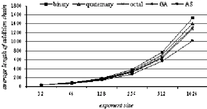
Figure 4: Comparison of the average length of the addition chains
exponents Ei + 1, Ei + 2, . . ., E + 2. In this case,
ant A may choose one of the exponent associated with
SMi+1,Ei−i, SMi+1,Ei−i+1, . . . , SMi+1,E−i+1. Further-more, antAchooses the new exponentEi+1with the prob-ability expressed through Eq. 8 below.
Pi,j=
SMi+1,j 2Ei−i−1
max
k=Ei−iSMi+1,k
if2Ei≤E &
j ∈[Ei−i,2Ei−i−1]
SMi+1,j E−i−1
max
k=Ei−iSMi+1,k
if2Ei> E&
j ∈[Ei−i, E−i−1]
0 otherwise
(8)
6 Performance Comparison
The ant system described in Algorithm 5 and Algorithm 6 was implemented using Java as a multi-threaded ant sys-tem. Each ant was simulated by a thread that implements the artificial ant computation of Algorithm 4. A Pentium IV-HTTMof a operation frequency of 1GH and RAM size of 2GB was used to run the ant system and obtain the per-formance results.
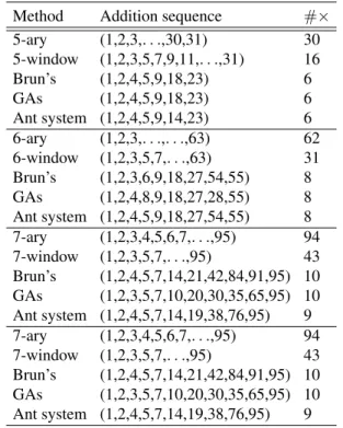
We compared the performance of m-ary methods, the Brun’s algorithm, genetic algorithms and ant system-based methods. The obtained addition chains are given in Table 1.
Table 1: The addition sequences yield for ξ(5,9,23),
ξ(9,27,55)andξ(5,7,95)respectively
Method Addition sequence #× 5-ary (1,2,3,. . .,30,31) 30 5-window (1,2,3,5,7,9,11,. . .,31) 16 Brun’s (1,2,4,5,9,18,23) 6 GAs (1,2,4,5,9,18,23) 6 Ant system (1,2,4,5,9,14,23) 6 6-ary (1,2,3,. . .,. . .,63) 62 6-window (1,2,3,5,7,. . .,63) 31 Brun’s (1,2,3,6,9,18,27,54,55) 8 GAs (1,2,4,8,9,18,27,28,55) 8 Ant system (1,2,4,5,9,18,27,54,55) 8 7-ary (1,2,3,4,5,6,7,. . .,95) 94 7-window (1,2,3,5,7,. . .,95) 43 Brun’s (1,2,4,5,7,14,21,42,84,91,95) 10 GAs (1,2,3,5,7,10,20,30,35,65,95) 10 Ant system (1,2,4,5,7,14,19,38,76,95) 9 7-ary (1,2,3,4,5,6,7,. . .,95) 94 7-window (1,2,3,5,7,. . .,95) 43 Brun’s (1,2,4,5,7,14,21,42,84,91,95) 10 GAs (1,2,3,5,7,10,20,30,35,65,95) 10 Ant system (1,2,4,5,7,14,19,38,76,95) 9
Table 2: Average length of addition sequence for Brun’s algorithm (BA), genetic algorithms (GA) and ant system (AS)
|Vp| BA GA AS
32 41 42 45
64 84 85 86
128 169 170 168 256 340 341 331 512 681 682 658 1024 1364 1365 1313
7 Conclusion
In this paper we applied the methodology of ant colony to the addition chain minimisation problem. Namely, we de-scribed how the shared and local memories are represented. We detailed the function that computes the solution fitness. We defined the amount of pheromone to be deposited with respect to the solution obtained by an ant. We showed how to compute the necessary probabilities and make the ade-quate decision towards a good addition chain for the con-sidered exponent.
Furthermore, we implemented the ant system described using multi-threading (each ant of the system was imple-mented by a thread). We compared the results obtained by the ant system to those ofm-ary methods (binary, quater-nary and octal methods). Taking advantage of the a previ-ous work on evolving minimal addition chains with genetic algorithm, we also compared the obtained results to those obtained by the genetic algorithm. The ant system always finds a shorter addition chain and gain increases with the size of the exponents.
References
[1] Rivest, R., Shamir, A. and Adleman, L., A method for Obtaining Digital Signature and Public-Key Cryp-tosystems, Communications of the ACM, 21:120-126, 1978.
[2] Dorigo, M. and Gambardella, L.M., Ant Colony: a Cooperative Learning Approach to the Travelling Salesman Problem, IEEE Transaction on Evolutionary Computation, Vol. 1, No. 1, pp. 53-66, 1997.
[3] Feber, J., Multi-Agent Systems: an Introduction to Distributed Artificial Intelligence, Addison-Wesley, 1995.
[4] Downing, P. Leong B. and Sthi, R., Computing Se-quences with Addition Chains, SIAM Journal on Com-puting, vol. 10, No. 3, pp. 638-646, 1981.
[5] Nedjah, N., Mourelle, L.M., Efficient Parallel Modular Exponentiation Algorithm, Second International Con-ference on Information systems, ADVIS’2002, Izmir, Turkey, Lecture Notes in Computer Science, Springer-Verlag, vol. 2457, pp. 405-414, 2002.
[6] Stutzle, T. and Dorigo, M., ACO Algorithms for the Travelling Salesman Problems, Evolutionary Algo-rithms in Engineering and Computer Science, John-Wiley & Sons, 1999.