Choosing Between Multinomial Logit and
Multinomial Probit Models for Analysis of
Unordered Choice Data
Jonathan Kropko
A Thesis submitted to the faculty of the The University of North Carolina at Chapel Hill in partial fulfillment of the requirements for the degree of Master of Arts in the Department of Political Science.
Chapel Hill 2008
Approved by:
George Rabinowitz, Advisor
Georg Vanberg, Member
Abstract
Choosing Between Multinomial Logit and Multinomial Probit Models for Analysis of Unordered Choice Data
Jonathan Kropko
(Under the direction of George Rabinowitz.)
Political researchers are often confronted with unordered categorical variables, such as
the vote-choice of a particular voter in a multiparty election. In such situations,
re-searchers must choose an appropriate empirical model to analyze this data. The two
most commonly used models are the multinomial logit (MNL) model and the multinomial
probit (MNP) model. MNL is simpler, but also makes the often erroneous independence
of irrelevant alternatives (IIA) assumption. MNP is computationally intensive, but does
not assume IIA, and for this reason many researchers have assumed that MNP is a
better model. Little evidence exists, however, which shows that MNP will provide more
accurate results than MNL. In this paper, I conduct computer simulations and show
that MNL nearly always provides more accurate results than MNP, even when the IIA
assumption is severely violated. The results suggest that researchers in the field should
Contents
List of Tables . . . . iv
Introduction . . . 1
Statistical Theory . . . 5
Multinomial Logit . . . 5
Multinomial Probit . . . 9
Methodology . . . 13
The Data Generating Process . . . 14
Error Correlation Structures and the IIA Assumption . . . 21
Strategic Voting . . . 24
Monte Carlo Simulations . . . 27
Evaluative Measures . . . 29
Results and Discussion . . . 31
Comparing MNL and MNP . . . 32
MNP Variance Estimation . . . 38
Conclusion . . . 42
Appendix . . . 43
List of Tables
1 Example Data from the Basic DGP. . . 16
2 Regression on Party Affect, Britian 1987. . . 19
3 Logistic Regression on Strategic Voting, Britian 1987. . . 26
4 Descriptive Statistics of Predicted Probability of Strategic Voting. . . 27
5 Simulation times. . . 31
6 Mean Evaluative Measures for MNL and MNP, Britain 1987 Model. . . . 32
7 Mean Evaluative Measures for MNL and MNP, Britain 1987 Model with Strategic Voting. . . 33
8 Mean Evaluative Measures for MNL and MNP, Basic Model. . . 34
9 Summary of the Results. . . 35
10 Mean Evaluative Measures for MNL and MNP, British Models, Omitting Large Variance Estimates. . . 41
11 Mean Evaluative Measures for MNL and MNP, Basic Models, Omitting Large Variance Estimates. . . 41
12 MNP Predictions for Alliance Variance and Correlation with Labour, Britain 1987 Models. . . 43
13 MNP Predictions for Alliance Variance and Correlation with Labour, Britain 1987 Models with Strategy. . . 44
Introduction
Sometimes, researchers in political science have to deal with an unordered, categorical
dependent variable. For example, in the study of elections, a dependent variable may
be the vote-choice of a particular voter. This dependent variable is categorical rather
than continuous: each choice or political party is another category. Furthermore, these
categories have no numerical label or natural ordering. Unordered, categorical dependent
variables appear in many other streams of political research, and more examples are not
hard to imagine.
Empirically, such variables can be modeled by using a probabilistic choice model, an
extension of a standard linear model, in which each choice is modeled with a separate
equation including the predictors and an error. There are many specific probabilistic
choice models, and two of the most widely used models are the multinomial logit (MNL)
and multinomial probit (MNP) models. Technically, these models are very similar: they
differ only in the distribution of the error terms. MNL has errors which are independent
and identically distributed according to the type-1 extreme value distribution, which
is also sometimes called the log Weibull distribution (see Greene (2000), p.858 for a
more detailed discussion of this distribution). MNP has errors which are not necessarily
independent, and are distributed by a multivariate normal distribution (Greene 2000,
p.856).
This difference between MNL and MNP may seem rather minor, but in practice
it has a big effect. The independent errors of MNL force an assumption called the
an individual’s evaluation of an alternative relative to another alternative should not
change if a third (irrelevant) alternative is added or dropped to the analysis. So if I
am twice as likely to vote for the Democratic Party than for the Republican Party, I
should remain twice as likely to vote Democrat over Republican if a third party becomes
a viable option. This assumption is not always a very good one in many situations. It
is easy to imagine that the Green Party becomes a more attractive choice to voters over
the Democrats if the Republicans drop out of the election, thus violating IIA. When IIA
is violated, MNL is an incorrectly specified model, and MNL coefficient estimates are
biased and inconsistent.
MNP does not assume IIA. In fact, an MNP model should estimate the error
cor-relations along with the coefficients. To that end, it may appear that MNP is a better
statistical model than MNL. Unfortunately, the situation is more complex.
A choice, or an alternative, is one category of the unordered, categorical dependent
variable. In the context of maximum likelihood estimation, a choice probability is a
formula to predict the probability that an individual chooses a certain alternative and
the likelihood function for such models is the product of the choice probabilities for each
individual. Choice probabilities in an MNL model are relatively simple, and computers
can maximize the resulting likelihood function almost instantaneously, even for a large
number of choices. For MNP, choice probabilities involve multiple integrals: as many
integrals as one fewer than the number of choices. Computers can typically maximize
likelihood functions with double or triple integrals, and may take a while to do so. But
when computers must deal with quadruple integrals, quintuple integrals, or even more
complicated integrals, MNP will often fail to converge or provide any useful estimation
at all. MNL, therefore, is a much more stable model. Instability in a statistical model
is a cause of concern.
Since MNP does not assume IIA it is often assumed to be more accurate than MNL.
strongly advocate the use of MNP as a less restrictive model, and focus their analysis
on a review of computational advances that might make MNP a more feasible model
for researchers. In the spirit of this argument, many researchers have used MNP to
analyze their choice data without considering MNL (Alvarez et al 2000 and Schofield
et al 1998, for example). Alvarez, Nagler, and Shaun Bowler (2000) justify MNP as
a model that “enabled us to study voter choices for the three major parties . . .
simultaneously and without restrictive and erroneous assumptions about the parties and
the electorate” (p.146). But I am concerned that although MNP does not assume IIA, it
loses accuracy at other points in its involved computation. The debate over whether to
use MNL or MNP has been framed as a debate of accuracy versus computational ease:
MNP provides more accurate results, but MNL converges much more quickly. There
is very little evidence, however, that proves that MNP really is more accurate than
MNL. Specifically, MNP may be an inefficient estimator, and there are situations in
which a biased and inconsistent estimator will be more accurate than a highly inefficient
estimator. Therefore, a direct comparison of MNL and MNP is in order.
Other researchers have already compared MNL and MNP models directly. Jay K.
Dow and James W. Endersby (2004) run a multinomial logit and a multinomial probit
model on data from U.S. and French presidential elections, and show that there is really
very little difference between the predictions of each model. All things being equal, they
conclude that MNL should be used over MNP. But Dow and Endersby only showed the
near equivalency of the two models for two very specific cases, and their results should
not be generalized. Kevin M. Quinn, Andrew D. Martin and Andrew B. Whitford (1999)
present two competing formal theories of vote choice in the Netherlands and Britain and
draw direct parallels to the competing MNL and MNP empirical models. They present
theory which suggests that IIA is a better assumption for the British data, and they
find that MNL is a better model for the British data while MNP should be a better
“depend crucially on the data at hand” (p.1231). This article suggests that empirical
models should be adjusted to correspond to the specifications of theoretical models.
But again, these conclusions are based on results from two datasets, so generalization is
problematic.
In order to be able to generalize results, MNP and MNL should be compared under
laboratory conditions. Specifically, I conduct a simulation study in which I generate
data while controlling the extent to which IIA holds or is violated. Such research was
conducted, but not published, by Alvarez and Nagler (1994). The research presented here
differs from their analysis in a few important ways: first, Alvarez and Nagler compare
MNP to an independent probit model in which all the covariances are constrained to
be zero. In this paper, I directly run MNL and MNP and compare the quality of the
estimations. Second, I use the British Election Study from 1987 as one model for the
data generating process (DGP). I also compare MNP and MNL in many more ways
which are of direct interest to political scientists, and I benefit from 13 years of advances
in computer processing power to perform simulations in many more cases.
I also consider the effect of strategic and sophisticated voting. In the simplest models
of voting, voters are sincere. That is, each voter will vote for the option she prefers most.
But these models are seldom effective at explaining or predicting what really happens
in elections. A voter casts a vote strategically when she votes for an option other than
her most preferred option in order to achieve a better outcome. Voters that may choose
to vote strategically are called sophisticated voters. Such voting behavior can cause the
IIA assumption to be violated. To demonstrate this fact, consider the simple example of
the 2000 presidential election. Very liberal voters sincerely would have preferred to vote
for Ralph Nader over Al Gore, and for Gore over George W. Bush. However, strategic
considerations moved many of these voters to vote for Gore in hopes of preventing the
election of Bush. For these voters, for strategic reasons, the probability of voting for Gore
alternative, is removed then they are much more likely to vote for Nader over Gore, thus
violating the IIA assumption. When strategic voting is present, MNL should perform
less accurately, but the effect on MNP is unclear. Many researchers have been interested
simultaneously in multinomial choices and strategic voting (Kedar 2005, Lawrence 2005,
Quinn and Martin 2002, Alvarez and Nagler 2000, Reed 1996, Abramson et al 1992),
so it is worthwhile to examine the effect of strategic voting on the performance of MNL
and MNP. Some of the simulations used for this project, described in section 3.3, are
designed to model and account for strategic voting.
My goal is to provide guidance to political researchers who must choose between these
two models. In this article, I report a surprising result: MNL gives more accurate point
estimates of coefficients than MNP, and also reports the correct sign and significance level
more frequently than MNP, even when the IIA assumption is severely violated. In all,
MNL outperforms MNP in all but the most severe violations of IIA. In the simulations
that model strategic voting, MNL always outperforms MNP. In the next section I will
discuss some of the statistical theory behind these two models. In section 3, I describe
the simulations in detail. In section 4, I provide the results and discuss the significance
of these results. In section 5 I conclude, and offer some thoughts about the benefits and
continuing disadvantages of MNL and other probabilistic choice models.
Statistical Theory
Multinomial Logit
The multinomial logit model has been the most commonly used model for analysis of
discrete choice data1 . MNL computes a different continuous latent variable for each
choice, and these variables are like evaluation scores of each individual for each choice:
the higher the score, the more likely that the individual chooses that alternative. So for
each choice j and individual i
Uij =βjxi+εij, (1)
where βjxi is the inner-product of the predictors and their coefficients for choice j, and
all of the εij are independent and identically distributed by the type 1 extreme value
distribution. In MNL, the predictors are fixed across choices, but the coefficients vary.
By fixed across choices, I mean that the value of a variable is the same no matter which
choice is being considered. Independent variables like age, gender, and income of a
respondent fit this description well.
Sometimes researchers find that interesting predictors vary across choices. For
ex-ample, the number of friends a voter has who are members of each party is not fixed
across choices. The conditional logit model was developed to account for such variables.
This model is similar to MNL, but the linear structure for the latent variable of choice
j takes the form
Uij =γzij +εij. (2)
Here, zij is an independent variable that varies across choices, and γ is the coefficient
for this predictor. Note that γ is itself fixed across choices. The logic here is that
variables that are different for each choice have the same effect across choices. So if
the ideological distance between an individual and each party is an important predictor
of that individual’s vote-choice, then distance is an equally important consideration
whether the Democrats, Republicans, or Greens are being considered. In an MNL
model, a predictor like religion is fixed across the choices, but the effect of the predictor is
different for each choice. So religion may be an important consideration of an individual
when they evaluate the Republican party, but may be less important when they evaluate
the Democrats or Greens.
developed a hybrid logit model. Under a hybrid model the latent variables take the form
Uij =βjxi+γzij +εij. (3)
In other words, a hybrid model simply combines MNL and conditional logit by adding
the two together in the deterministic part of the model.
For all of these models, the dependent variable takes the form:
yi =
1 if max (Ui1, Ui2, . . . , Uim) =Ui1,
2 if max (Ui1, Ui2, . . . , Uim) =Ui2,
...
m if max (Ui1, Ui2, . . . , Uim) =Uim.
(4)
So a voter chooses the alternative that they evaluate most highly.
Remember that in binary logit models all the coefficients describe the relative
proba-bility of the positive outcome (choice 1) to the negative outcome (choice 0). Here, choice
0 acts as a base for the coefficients. In MNL, MNP, and in multinomial models with
choice-fixed predictors in general, the coefficients do the same thing: they describe the
relative probability of a choice to a base-choice. Therefore, if there are M choices, MNL
and MNP will provide M −1 sets of coefficients, setting the coefficients for the
base-choice all equal to zero. This base is chosen arbitrarily, and can easily be changed in a
statistical package such as Stata. For conditional logit, this normalization of coefficients
is unnecessary because conditional logit only estimates one set of coefficients. For the
hybrid model, only the coefficients which vary across choices (the MNL part) need to be
set to zero for the base-case.
choice 1 as the base, the odds ratio for any other choice j is
P(yi =j)
P(yi = 1)
=eβjxi. (5)
The choice probability for the base is:
P(yi = 1) =
1
1 +PNj=2eβjxi, (6)
and the choice probability for any other choice k is:
P(yi =k) =
eβkxi
1 +PNj=2eβjxi. (7)
Technically, IIA assumes independence of the errors in the evaluation functions, but an
important effect of this assumption is that the odds ratios are fixed when other choices
are added or dropped. Notice one important thing about the odds ratio for MNL:
equation 5 only depends on the coefficients for choice j. No change to any other choice’s
coefficients will change this ratio. This feature of MNL is the independence of irrelevant
alternatives assumption (IIA) in action. Although the odds ratios for the conditional
logit and hybrid models take slightly different forms, these models assume IIA as well.
So the relative probability that I choose choice a over choice b should not be affected if
choice c is no longer an option. There are many cases in which IIA is simply not true.
When IIA is a false assumption, the estimations of these logit models are biased and
inconsistent: serious problems.
It can be shown that the choice probabilities for MNL described in equation 7 are
closed-form precisely because the errors are independent. Therefore the definition of IIA
as error independence is exactly equivalent to the definition as odds ratios being fixed
to additions and deletions of other choices.
model. So I compare the hybrid model to the probit equivalent of the hybrid model. I
generate data with both choice-fixed and choice-specific predictors. So from this point
onward, when I refer to the MNL model, I am referring to the hybrid logit model and
when I refer to the MNP model I am referring to the probit equivalent to the hybrid
logit model.
Multinomial Probit
The advantage of MNP over MNL is that MNP does not assume IIA. The obvious
disadvantage is that MNP is far more computationally intensive. For each choice j the
evaluation functions are
Uij =βjxi+γzij +εij, (8)
which are analogous to the evaluation functions for the hybrid logit model. But here,
the errors εi1, . . . , εiM are distributed by a multivariate normal distribution in which
each error has a mean of zero and the errors are allowed to be correlated. The choice
probabilities using MNP are very, very complex. Let Vij represent the deterministic part
of Uij for each choicej, so thatUij =Vij+εij. Consider the simple case of three choices.
For notational ease, let ηi2 =εi2−εi1 and ηi3 =εi3−εi1. The probability of choosing
alternative 1 is the probability that Ui1 is the highest evaluation2 :
P(yi = 1) =P(Ui1 > Ui2 and Ui1 > Ui3) (9)
=P(Vi1+εi1 > Vi2+εi2 and Vi1+εi1 > Vi3+εi3) (10)
=P(ηi2 < Vi1−Vi2 and ηi3 < Vi1−Vi3) (11)
=
Z Vi1−Vi2
−∞
Z Vi1−Vi3
−∞
f(ηi2, ηi3)dηi3dηi2, (12)
where f(ηi2, ηi3) is the joint probability density function (PDF) of ηi2 and ηi3. In this
case, the PDF is a multivariate normal distribution, a notoriously difficult function to
integrate. In general, computers have a difficult time computing or estimating multiple
integrals. But choice probability formulas in MNP with N alternatives involve (N −
1)tuple integrals.
Binary probit models are under-specified in that we cannot simultaneously estimate
the coefficients and the variance of the errors. Therefore, we assume that the error
variance is 1 and estimate the coefficients using this normalization. In effect, we are
dividing all the coefficients by the standard deviation of the errors. But then we are
really estimating βσ rather than β, so we cannot trust the direct point estimates from
a binary probit model. Multinomial probit models make a similar normalization: they
constrain one of the variances in the differenced variance-covariance matrix3 . So, in the
choice probability described above, the variance-covariance matrix of η2 = ε2 −ε1 and
η3 =ε3−ε1 is
σ
2
η2 .
ση2,η3 σ2η3
, (13)
where
ση22 =V(ε2−ε1) =V(ε2) +V(ε1)−Cov(ε2, ε1)
=σε21 +σε22 −ρε1,ε2σε1σε2. (14)
Similarly,
σ2
η3 =σ
2
ε1 +σ
2
ε3 −ρε1,ε3σε1σε3. (15)
And the covariance is
ση2,η3 =E
·¡
η2−E(η2)
¢¡
η3−E(η3)
¢¸
=E(η2η3) (16)
=E[(ε2−ε1)(ε3−ε1)] (17)
=E(ε2ε3)−E(ε2ε1)−E(ε3ε1) +E(ε2
1) (18)
=ρε2,ε3σε2σε3 −ρε1,ε2σε1σε2 −ρε1,ε3σε1σε3+σ
2
ε1. (19)
MNP only requires that one variance in the differenced variance-covariance matrix in
equation 13 be constrained to some constant value. The “asmprobit” routine in Stata
makes normalizations which are more restrictive4 . In order to ensure that σ2
η2 is
con-strained to be constant, “asmprobit” constrains the variance of both the first and second
choice to be 1, and every correlation involving the first choice to be zero (Statacorp 2007):
σ2
ε1 = 1, σ
2
ε2 = 1, (20)
ρε1,ε2 = 0, ρε1,ε3 = 0, (21)
which implies that
σε1,ε2 =ρε1,ε2σε1σε2 = 0, (22)
σε1,ε3 =ρε1,ε3σε1σε3 = 0, (23)
σε2,ε3 =ρε2,ε3σε2σε3 =ρε2,ε3σε3. (24)
Then the variance-covariance matrix of (ε1, ε2, ε3)0 used by the “asmprobit” command
is σ2
ε1 . .
σε1,ε2 σ
2
ε2 .
σε1,ε3 σε2,ε3 σ
2 ε3 =
1 . .
0 1 .
0 ρε2,ε3σε3 σ
2 ε3
, (25)
so the variance-covariance matrix of (η2, η3)0 becomes
2 .
ρε2,ε3σε3 + 1 1 +σ
2
ε3
. (26)
Therefore, in the three choice case, the only elements of the error covariance structure
estimated by the “asmprobit” command are the variance of the third choice (σ2
ε3) and
the correlation between the second and third choices (ρε2,ε3). These two parameters are
estimated along with the coefficients. Unfortunately, as is shown later in this paper,
these estimates are rarely very accurate or useful.
The likelihood functions for multinomial logit and multinomial probit differ only in
the formulation of the choice probabilities. Let
λij =
1 if yi =j,
0 if yi 6=j.
(27)
Then the likelihood function is
L= N Y i=1 M Y j=1
P(yi =j)λij, (28)
which is maximized with respect to the coefficients, and in the case of MNP, the
uncon-strained variances and covariances. For the logit models, the choice probability inside
the double-product is straight forward, so these models are computed quickly. But for
MNP this function is extremely complex. There are simulation methods to approximate
of MNP is used, a powerful computer and patience are both necessary.
For MNP, standard maximum likelihood estimation of the likelihood function will
fail to converge. Stata and other statistical packages use instead simulated maximum
likelihood techniques. In essence, the choice probabilities on the MNP model are
esti-mated using a technique involving random draws and monte carlo estimation. The most
common simulated maximum likelihood technique is the Geweke-Hajivassiliou-Keane
(GHK) algorithm (Geweke 1991, Keane 1990, Keane 1994, Hajivassiliou and McFadden
1998, Hajivassiliou, McFadden and Ruud 1996), which is the algorithm used by the Stata
“asmprobit” command (Statacorp 2007). I suspect that MNP loses some efficiency in
the simulated maximum likelihood estimation. In this paper, I test whether this
compu-tational disadvantage of MNP causes MNP to be less accurate than biased MNL, even
when IIA is a highly erroneous assumption. I do not delve into the exact specifications of
the GHK algorithm to find its deficiencies; instead I compare the final results of the two
models since few researchers in political science are concerned with the details of GHK
estimation, but many are concerned with the performance of MNP generally. Identifying
the precise areas in which GHK may lose accuracy and fixing those deficiencies is an
agenda for future research.
As the number of alternatives increases, the complexity of the choice probabilities in
MNP increases drastically. Therefore, we can expect that MNP is more efficient when
there are fewer choices. But I find that MNL outperforms MNP even in the simple
three-alternative case, which should raise serious concerns about the utility of MNP models
for political science research in general.
Methodology
Suppose we knew the true values of the parameters to be estimated by MNL and MNP.
they return point estimates of the coefficients5 . But such a methodology is working
backwards: typically we use a model to estimate the truth; here, we use the truth to
evaluate the model.
The Data Generating Process
If we start with the true values of the parameters, then it may not matter what values
these parameters take. The important point is how well each model returns these values.
The means through which the “true” data is obtained is called a data generating process
(DGP). Often, some stochastic algorithm is used. Alvarez and Nagler (1994), for
ex-ample, generate independent variables using a uniform number generator, and multiply
each predictor by an arbitrarily chosen coefficient. Here, I choose to model the DGP in
two ways: one after data from the 1987 British Election Study and one in the style of
Alvarez and Nagler. I call the models that use the British data to model the DGP the
“British” models, and I call the models that generate the data uniformly the “basic”
models. The basic models are simpler, but the data do not resemble any real political
data that researchers in the field may encounter. In contrast, the 1987 British election
survey dataset has been used in a number of important papers on multinomial choice
methodology (Whitten and Palmer 1996, Alvarez and Nagler 1998, Quinn, Martin and
Whitford 1999, for example). Using real data to model the DGP places the comparison
within the realm of very real current research, so the results should be more immediately
useful for researchers in the field.
Theoretically, the latent variables in a probabilistic choice model represent the utility
an individual has for each alternative. I model these latent equations in each DGP.
The latent variables are the sum of two parts: the deterministic part derived from the
variables and their coefficients, and a stochastic error. Data is arranged in the form of a
person-choice matrix, in which one observation is identified by the voter and the choice
(Conservative, Labour, or Alliance) being considered. In each multinomial model, one
choice must be designated as the base choice. Both MNL and MNP make the same
standardization; they essentially set the coefficients on the choice-fixed predictors all
equal to zero for the base choice. For the choice-fixed variables, the coefficients describe
the effect of the variable on a voter’s evaluation of choices 2 and 3 (Labour and the
Alliance) relative to their evaluation of choice 1 (Conservative).
Basic Models
In the basic models, the coefficients and the data are randomly drawn from a uniform
distribution. One randomly generated independent variable is allowed to vary across
choices, and another independent variable and a constant are fixed across choices. Since
the data generated here are completely artificial, I refer to the alternatives simply as
choice 1, choice 2, and choice 3. I set choice 1 as the base choice.
The choice-variant data,z, are independently drawn from a uniform distribution from
0 to 1. x is also drawn from a uniform distribution from 0 to 1, but x is held constant
for different alternatives within the observations for each individual. The errors, ε1, ε2,
and ε3 are randomly drawn from a trivariate normal distribution with means 0:
εi,1
εi,2
εi,3
∼N
µ ·
0 0 0
¸0
,Σ
. (29)
The different structures of the variance-covariance matrix of these errors, denoted by
Σ, are crucial to the theoretical goals of the simulations. I discuss the error structures
more thoroughly in section 3.2. In these basic models, the variances of the choice errors
are all set at one, but the covariances vary as an experimental control. The errors must
be drawn independently for each individual, but jointly across the alternatives for each
Five coefficients (λ,β2,0,β2,1,β3,0, and β3,1) are independently drawn from a uniform
distribution from−1 to 1 before each iteration of MNL and MNP estimation. MNL and
MNP will provide estimates of these five randomly generated coefficients. The variable
U contains the latent utilities of each individual for each choice. The simulated vote
choice of each individual is the alternative with the highest value of U. For the basic
DGP, the evaluation of individual i of choice 1 is
Ui,1 =λzi,1+εi,1. (30)
The evaluation of choice 2 is
Ui,2 =λzi,2+β2,1xi+β2,0+εi,2, (31)
and the evaluation of choice 3 is
Ui,3 =λzi,3+β3,1xi+β3,0+εi,3. (32)
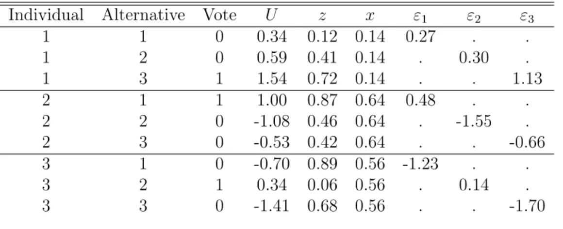
As an example, the generated dataset may look like the data in the table 1. We can
Table 1: Example Data from the Basic DGP.
Individual Alternative Vote U z x ε1 ε2 ε3
1 1 0 0.34 0.12 0.14 0.27 . .
1 2 0 0.59 0.41 0.14 . 0.30 .
1 3 1 1.54 0.72 0.14 . . 1.13
2 1 1 1.00 0.87 0.64 0.48 . .
2 2 0 -1.08 0.46 0.64 . -1.55 .
2 3 0 -0.53 0.42 0.64 . . -0.66
3 1 0 -0.70 0.89 0.56 -1.23 . .
3 2 1 0.34 0.06 0.56 . 0.14 .
3 3 0 -1.41 0.68 0.56 . . -1.70
into Stata:
xi: clogit vote z i.alternative i.alternative|x, group(individual)
The “clogit” command runs a conditional logit model which considers independent
vari-ables like z that vary across alternatives. The “xi” and “i.” commands instruct Stata
to break the categorical variable “alternative” into dummy variables for each category.
Choice 1 is omitted as the base alternative. This model provides a coefficient estimate on
z which will be compared to the known, true coefficientλ. The model also provides
co-efficient estimates on dummy variables for choice 2 and choice 3, comparable to the true
coefficients β2,0 and β3,0, and on these dummy variables interacted with x, comparable
to the true coefficients β2,1 and β3,1.
To run a multinomial probit model, we enter the following command:
asmprobit vote z, case(individual) alternatives(alternative)
casevars(x)
In order to run a multinomial probit model, we must specify the cases, individuals in this
case, and the alternatives, contained in the variable named “alternative.” Variables like
x that are fixed across alternatives must be specified within the “casevars” option. The
multinomial probit model provides estimates of the same coefficients that the hybrid
multinomial logit model does.
We must account for the normalization that is made for the probit estimates that is
not made for the logit estimates. The way I account for the standardized coefficients is
described in section 3.5. After fixing the coefficients, they are comparable to the true
parameters in exactly the same way, and we can directly see which model returned the
British Models
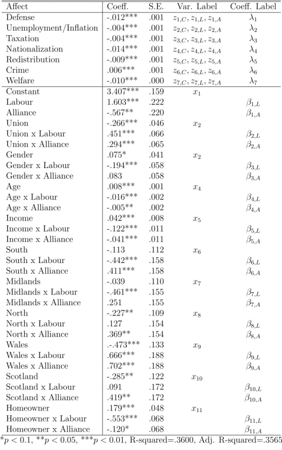
To obtain realistic coefficients for the British DGP, I run a regression on affect, or the
affinity a person has for each party, using the 1987 election data. For this regression,
the data is set up in the same way as in the basic model. Here, however, we estimate
a greater number of parameters. In this setup, the dependent variable is the affect of
an individual for each party. Choice-specific variables such as ideological distance are
treated as regular regressors. Choice-fixed variables such as the respondent’s age and
gender are multiplied by dummy variables for each (non-base) choice so that the effect
of that variable on the affect for each choice can be derived. Below I present the results
from this regression6 . For the British models I use the data from a sample of real
British voters consisting of 2440 respondents after dropping observations with missing
values, and the corresponding coefficients from the regression in table 27 . Conservative
is the base choice. For the choice-fixed variables, the coefficients describe the effect of
the variable on a voter’s evaluation of Labour or the Alliance relative to their evaluation
of the Conservative party.
For individual i, the evaluation of the Conservative party is
Ui,C =
7
X
k=1
λkzi,k,C +εi,C, (33)
6The coding of these variables is as follows: affect is v13a when the choice is Conservative, v13b when the choice is Labour, and the average of v13c and v13d when the choice is Alliance. Labour and Alliance are dummy variables that equal 1 when v8a=2 and 3 respectively. Defense distance through welfare distance are squared differences between the individual’s self placement on the issue (v23a, v28a, v29a, v34a, v35a, v39a, v40a) and the means over all respondents for the party position on each issue (parts b, c, and d of the same question). Union is a dummy that equals 1 if v49c=1 or 2, and 0 if v49c=0. Gender is v58b, age is v58c, and income is v64. The regional variables south through scotland are dummy variables derived from v48. Homeowner is a dummy that equals 1 if v60ab=02, and 0 otherwise.
Table 2: Regression on Party Affect, Britian 1987.
Affect Coeff. S.E. Var. Label Coeff. Label
Defense -.012*** .001 z1,C, z1,L, z1,A λ1
Unemployment/Inflation -.004*** .001 z2,C, z2,L, z2,A λ2
Taxation -.004*** .001 z3,C, z3,L, z3,A λ3
Nationalization -.014*** .001 z4,C, z4,L, z4,A λ4
Redistribution -.009*** .001 z5,C, z5,L, z5,A λ5
Crime .006*** .001 z6,C, z6,L, z6,A λ6
Welfare -.010*** .000 z7,C, z7,L, z7,A λ7
Constant 3.407*** .159 x1
Labour 1.603*** .222 β1,L
Alliance -.567** .220 β1,A
Union -.266*** .046 x2
Union x Labour .451*** .066 β2,L
Union x Alliance .294*** .065 β2,A
Gender .075* .041 x2
Gender x Labour -.194*** .058 β3,L
Gender x Alliance .083 .058 β3,A
Age .008*** .001 x4
Age x Labour -.016*** .002 β4,L
Age x Alliance -.005** .002 β4,A
Income .042*** .008 x5
Income x Labour -.122*** .011 β5,L
Income x Alliance -.041*** .011 β5,A
South -.113 .112 x6
South x Labour -.442*** .158 β6,L
South x Alliance .411*** .158 β6,A
Midlands -.039 .110 x7
Midlands x Labour -.461*** .155 β7,L
Midlands x Alliance .251 .155 β7,A
North -.227** .109 x8
North x Labour .127 .154 β8,L
North x Alliance .369** .154 β8,A
Wales .-.473*** .133 x9
Wales x Labour .666*** .188 β9,L
Wales x Alliance .702*** .188 β9,A
Scotland -.285** .122 x10
Scotland x Labour .091 .172 β10,L
Scotland x Alliance .419** .172 β10,A
Homeowner .179*** .048 x11
Homeowner x Labour -.553*** .068 β11,L
Homeowner x Alliance -.120* .068 β11,A
for the Labour party
Ui,L =
7
X
k=1
λkzi,k,L+
11
X
j=1
βj,Lxi,j+εi,L, (34)
and for the Alliance
Ui,A =
7
X
k=1
λkzi,k,A+
11
X
j=1
βj,Axi,j+εi,A. (35)
Once again, εi,C, εi,L, and εi,A are randomly generated from a trivariate normal
distribution with means equal to zero and a predefined variance-covariance structure.
The variances of the errors are not equal to zero in the British models. Instead, the value
of each variance is derived from the data. Again, that process is described in detail in
section 3.2. The correlations, however, vary in the same way as in the basic models.
Unless strategic voting is being considered (section 3.3), the simulated vote-choice of
individual iis simply the alternative with the highest associated utility. For the British
models:
˜
yi =
Conservative if max (Ui,C, Ui,L, Ui,A) =Ui,C,
Labour if max (Ui,C, Ui,L, Ui,A) =Ui,L,
Alliance if max (Ui,C, Ui,L, Ui,A) =Ui,A.
(36)
In other words, if individual iis voting sincerely, then she chooses to vote for the party
she evaluates most highly. With a known error variance structure, I have now generated
a dependent variable which can be analyzed using MNL and MNP. The results from
MNL and MNP can now be directly compared to the true values of the parameters
Error Correlation Structures and the IIA Assumption
IIA holds precisely when there is no covariance between the errors in Σ. Here I choose
formulations of Σ to consider in the simulations. I consider cases that span the spectrum
of the validity of IIA: in one case IIA holds perfectly, but in others IIA becomes an
increasingly bad assumption.
In the regression presented in table 2, the “natural” variance-covariance and
corre-lation matrices for εi,C, εi,L, and εi,A can be derived. Recall that the data is in the
form of a person-choice matrix, in which each observation is uniquely defined by the
individual and the choice being considered by that individual. So individual i receives
three observations in the data: one where individual iconsiders the Conservative party,
one where Labour is considered, and one where the Alliance is considered. Predicted
residuals are calculated and are separated into three new variables: one for each of the
three choices. The natural variance-covariance matrix is the variance-covariance matrix
of these three parts of the predicted residuals. Specifically:
Σnatural =
1.133 . .
−0.406 1.127 .
−0.083 −0.039 0.604
, (37)
where 1.133 is the variance of the residuals of observations in which voters consider the
Conservative party, 1.127 is the variance of the residuals of observations in which voters
consider the Labour party, and 0.604 is the variance of the residuals of observations in
which voters consider the Alliance. Σnatural yields the correlation matrix
χnatural =
1 . .
−0.359 1 .
−0.100 −0.047 1
So the unobserved predictors of affect on the Conservative and Labour parties are
strongly and negatively correlated. The unobserved predictors of affect on the
Conser-vative party and the Liberal-Social Democrat Alliance are negatively but more modestly
correlated, and Labour and the Alliance are nearly independent.
In order to model the simulated data as closely as possible after the 1987 British
election, I use these natural variances in each experimental variance-covariance matrix
in the models described below. So for each experimental case in the British models
Σ =
1.133 . .
σC,L 1.127 .
σC,A σL,A 0.604
. (39)
For the basic models, we use
Σ =
1 . .
σ1,2 1 .
σ1,3 σ2,3 1
, (40)
where for each model, for choices a and b,
σa,b =ρa,b
p
σ2
a
q
σ2
b. (41)
Here, the variances σ2
a and σ2b are the known constants listed above which are specific
to each DGP, and ρa,b is the correlation between errors for choices a and b. So, for the
British models
σC,L =ρC,L×
√
1.133×√1.127 = 1.13ρC,L, (42)
σC,A =ρC,A×
√
1.133×√0.604 = 0.83ρC,A, (43)
σL,A=ρL,A×
√
and for the basic models
σ1,2 =ρ1,2×
√
1×√1 = ρ1,2, (45)
σ1,3 =ρ1,3×
√
1×√1 = ρ1,3, (46)
σ2,3 =ρ2,3×
√
1×√1 = ρ2,3. (47)
The correlations are directly indicative of the validity of the IIA assumption, so I only
need to alter these correlationsρa,b. I consider 11 models, which I call modelsA through
K:
χA =
1 . .
0 1 .
0 0 1
, χB =
1 . .
.10 1 .
.10 .10 1
, (48)
χC =
1 . .
.25 1 .
.25 .25 1
, χD =
1 . .
.50 1 .
.50 .50 1
,
χE =
1 . .
.75 1 .
.75 .75 1
, χF =
1 . .
0 1 .
.80 0 1
,
χG=
1 . .
0 1 .
−.80 0 1
, χH =
1 . .
0 1 .
.50 .80 1
χI =
1 . .
0 1 .
−.50 .80 1
, χJ =
1 . .
−.20 1 .
−.50 .80 1
,
χK =
1 . .
−0.359 1 .
−0.100 −0.047 1
.
Models A, F, G,H, I, and J were considered by Alvarez and Nagler (1994). Models E
through J probably set the correlations at levels higher than anything researchers are
likely to see in reality, but it is important to observe the behavior of the multinomial
choice models in the case of extreme violation of IIA. Notice that the correlation matrix
for model K is precisely the same as the natural correlation matrix presented above.
Since these variances come directly from real data, the results for modelK are probably
the most directly applicable to applied research.
In order to generate the simulated data, I first use a random number generator to
drawεi,1,εi,2, andεi,3 ( orεi,C,εi,L, and εi,A) for each observation. The random number
generator draws from a trivariate normal distribution as defined above, with means 0 and
variance-covariance matrix Σ specified by one of the models A through K. Therefore,
the correlations are defined first, and the correlated errors are then passed to the DGP.
Strategic Voting
As discussed earlier, one reason why IIA may be an inappropriate assumption for many
elections is the presence of strategic voting. MNL and MNP work the same way in
considering strategic voting. For MNL and MNP the evaluation equations Ui,C, Ui,L,
and Ui,A have two parts: a deterministic part composed of the predictors and their
coefficients, and the stochastic errors which represent the unexplained variance. Neither
the other choices8 . A voter’s evaluation of the Ralph Nader and the Green Party in
the 2000 U.S. Presidential Election, for example, probably depended on the strength of
the two major parties and their candidates in the voter’s state. In close elections, very
liberal voters were often compelled to vote for the Democratic Party over the Green
Party, against their sincere preferences, in order to help defeat the Republican Party.
But predictors in these MNL and MNP models depend only on the voter and the choice
and not on other choices. Therefore, violations of IIA and strategic voting cannot be
accounted for by the deterministic parts of these models. MNL assumes independence
of the errors, so there is no way whatsoever to model strategy in an MNL model. MNP
may reflect strategy in the unexplained variance of the model. Therefore, theoretically,
the presence of strategic voting should improve the performance of MNP relative to
MNL.
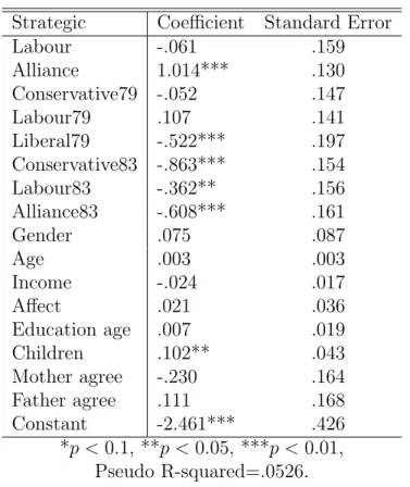
In the data from the 1987 British election, voters were asked why they voted the
way they did. Many of the voters gave answers which reflected strategic considerations9
. These respondents were then asked which party they really preferred10 . I generate a
binary indicator variable which equals one when a respondent votes for a party other than
her most preferred one. This indicator is not a particularly exact measure of strategic
voting in and of itself, but it does provide a useful way to gage the performance of MNL
and MNP when voters do not vote for their first choice. I run a binary logistic model
on the indicator for a strategic vote. I use a number of predictors which seem to make
8Theoretically, the model can account for strategic voting by controlling for it as a predictive variable. Whether or not a person votes strategically, however, is not typically observable. Survey respondents will not always admit to voting strategically, and proxies for strategic voting are not likely to be exact. In fact, most multinomial models of vote choice make no attempt to account for strategic voting in the deterministic part of the model. For example, none of the articles listed above which use the 1987 British election data consider strategy. Failing to include strategic voting in the model specification leaves only the stochastic components to account for the variance generated by strategic voting.
9Variable v9a gives voter responses to the question “which comes closest to the main reason you voted the way you did?” 211 respondents answered “preferred party had no chance of winning,” 18 answered “voted against party(ies) or candidate,” and 6 responded “tactical voting.”
some sense11. My intention is to create a measure for each respondent of the probability
of a strategic vote in the British models. Since these probabilities will be used to alter
artificial data, I am not overly concerned with the correct theoretical specification of
this model. I report the results of this binary logistic regression in table 3 below.
Table 3: Logistic Regression on Strategic Voting, Britian 1987.
Strategic Coefficient Standard Error
Labour -.061 .159
Alliance 1.014*** .130
Conservative79 -.052 .147
Labour79 .107 .141
Liberal79 -.522*** .197
Conservative83 -.863*** .154
Labour83 -.362** .156
Alliance83 -.608*** .161
Gender .075 .087
Age .003 .003
Income -.024 .017
Affect .021 .036
Education age .007 .019
Children .102** .043
Mother agree -.230 .164
Father agree .111 .168
Constant -2.461*** .426
*p < 0.1, **p <0.05, ***p < 0.01, Pseudo R-squared=.0526.
Again, this model is not a particularly good one by most standards. Many of the
predictors fail to be significant. But the model will provide a rudimentary measure of the
probability of a strategic vote for the purposes of the simulation. This variable, which I
denoteπ, is summarized in table 4 below. On average, a voter will vote strategically 8.6
percent of the time. Of 2440 voters then, we expect about 210 strategic votes. Certainly
this change is enough to affect the estimations of MNL and MNP.
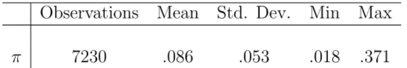
Table 4: Descriptive Statistics of Predicted Probability of Strategic Voting.
Observations Mean Std. Dev. Min Max
π 7230 .086 .053 .018 .371
In the British model simulations, I generate a variableδ that contains random
num-bers generated from a uniform distribution between 0 and 1. For an individual, ifδ < π,
the voter chooses their second highest evaluation instead. Mathematically,
(˜yi|δ < π) =
max(L,A)(Ui,L, Ui,A) if max (Ui,C, Ui,L, Ui,A) = Ui,C,
max(C,A)(Ui,C, Ui,A) if max (Ui,C, Ui,L, Ui,A) = Ui,L,
max(C,L)(Ui,C, Ui,L) if max (Ui,C, Ui,L, Ui,A) = Ui,A.
(49)
In the case where an individual evaluates two parties equally higher than the other party,
one of the parties is randomly selected as the first choice and the other is the second
choice. For the British DGP models, each simulation for error models A through K is
run twice, once without strategic considerations where the dependent variable is defined
as in equation 36, and once with strategic considerations where the dependent variable
is defined as in equation 49. I also run simulations for models Athrough K with a basic
DGP model. I run 33 simulations in all.
Monte Carlo Simulations
Each simulation consists of 100 iterations of the same procedure. I run each of these
simulations on Stata Version 10.0, Special Edition12. Below I summarize the simulation
process, step by step:
• The data are generated:
– For the British DGP models, the coefficients and covariates are saved from the regression on party affect in table 2 and are therefore the same from
iteration to iteration throughout the simulation. For the basic models, the
coefficients and covariates are all drawn from uniform distributions before
each iteration13 .
– New errors are generated during each iteration. The errors are random num-bers drawn from a multivariate normal distribution with means zero and a
variance-covariance structure defined by one of the models A through K14 .
– The latent evaluation variables for each choice are generated from the formulas described in equations 30, 31, and 32 for the basic models and 33, 34, and
35 for the British models. Because the errors are stochastic, the simulated
vote-choice should be slightly different from iteration to iteration.
– The British models are each run once with strategic considerations and once without them. If strategic voting is not being considered, then the simulated
vote-choice is the highest evaluation of the three latent variables defined in
equations 33, 34, and 35. If strategic voting is being considered, a voter still
votes for their highest evaluated party unless they are selected as strategic,
in which case they vote for their second-highest evaluated party. Because the
13The random number generator in Stata is really aquasirandom number generator. Given a number as a seed, Stata will use an algorithm to produce a string of numbers from that seed that resemble random numbers. But Stata uses a default seed which produces the same “random” numbers whenever Stata is launched. At first I was generating the same exact numbers from simulation to simulation, which was severely biasing my results. It is important to change the random seed from simulation to simulation when doing Monte Carlo work in Stata. I suggest generating a string of random numbers and setting the new random seed to the next number in that list for each simulation. The Stata manual (Statacorp. 2007) provides a detailed discussion of this quasi-random number generator.
strategic draws are stochastic, the voters who are selected as strategic should
vary from iteration to iteration.
• An MNL and MNP model is run on the simulated data. The simulated vote-choice
is the dependent variable.
• The coefficient point estimates and p-values from these models are saved as well as
the estimates from MNP of the unconstrained elements of the variance-covariance
matrix.
Evaluative Measures
The estimates from MNL and MNP are then evaluated for their accuracy compared to
the true model. One problem, described in section 2.2, is that probit models standardize
the base variances, so coefficients are all scaled by a normalized variance parameter. If
the true parameter to be estimated is β, then MNL provides a direct estimate ofβ, but
MNP provides a scaled coefficient estimate that takes the form βσ. In order to directly
compare MNL and MNP point estimates I divide each coefficient estimate from MNL,
MNP, and the true model by the mean of the absolute values of the coefficient estimates
from that model. I use the absolute values in order to preserve signs. Suppose there are
M coefficients returned by the models, then for MNP
β1 σ
ÁPM j=1(|
βj
σ|)
M (50)
= β1
σ
Á1
σ
PM
j=1(|βj|)
M (51)
= β1
σ
ÁPM
j=1(|βj|) M
1
σ (52)
=β1
ÁPM
j=1(|βj|)
which can be directly compared to corresponding measures from MNL and the true
model since the variances from probit have been canceled out.
I use three measures to compare MNL and MNP.
• Measure 1. The scaled coefficients for MNL and MNP are compared against the scaled, true coefficient values. Accuracy is assessed for each model using a
mean squared error measurement. The lower this measurement, the closer a model
returns the true coefficient estimates.
• Measure 2. Coefficients in multinomial choice models are usually interpreted for their signs and not their magnitudes. Estimates that switch the sign are therefore
very poor estimates. MNL and MNP are compared using the percent of successful
returns of coefficient signs. In the British models, the percent itself is reported.
There are only five coefficients to estimate in the basic models, so the average
number correct out of five is reported.
• Measure 3. For the British models, the regression coefficients in table 2 are either significant at the .1 level or are insignificant at that level. Likewise, MNL and MNP
coefficient estimates are either significant or insignificant at the .1 level. I say that
the MNL or MNP coefficient estimate returns the correct significance level if it
is significant when the corresponding true coefficient is significant, or insignificant
when the corresponding true coefficient is insignificant. For the British models only,
MNL and MNP are compared using the percent of correct statistical inferences.
In the basic models, the randomly generated coefficients have no standard errors.
Therefore, there is no baseline of significance against which to compare MNL and
MNP, so this third measure is omitted for the basic models.
For each of these three measures, I report the means for each of the 33 simulations over
MNL and MNP for each simulation. The results are reported below. I also saved the
unconstrained MNP estimates for the parameters in the variance-covariance matrix.
Results and Discussion
The simulations, which each performed 100 iterations of data generation and MNL and
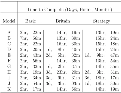
MNP estimation, varied widely in their running times15 . These simulation times are
listed in table 5. The basic models ran more quickly because they involved the estimation
of fewer parameters than the British models.
Table 5: Simulation times.
Time to Complete (Days, Hours, Minutes)
Model Basic Britain Strategy
A 2hr, 22m 14hr, 19m 13hr, 19m
B 7hr, 56m 13hr, 39m 15hr, 24m
C 2hr, 22m 16hr, 30m 15hr, 18m
D 2hr, 20m 1d, 8hr, 40m 15hr, 24m
E 2hr, 43m 2d, 5hr, 32m 1d, 9hr, 47m
F 2hr, 56m 14hr, 35m 13hr, 54m
G 3hr, 32m 1d, 2hr, 37m 14hr, 35m
H 3hr, 19m 3d, 23hr, 20m 2d, 3hr, 31m I 2hr, 34m 3d, 9hr, 31m 3d, 18hr, 17m J 2hr, 54m 3d, 3hr, 03m 1d, 18hr, 30m
K 2hr, 17m 14hr, 56m 14hr, 19m
Comparing MNL and MNP
The results of the simulations are presented in table 6 for the British models, in table
7 for the British models with strategy, and in table 8 for the basic models. In table
8, sign is the average number coefficient signs correctly estimated out of 5. For each
error correlation model A through K, the reported evaluative measures are the means
over 100 iterations. The columns labeled ∆ are the values for MNP subtracted from the
values for MNL. For point accuracy, lower values are better, so negative values of the
difference indicated that MNL performs better than MNP, and positive values indicate
that MNP performs better than MNL. For sign and significance accuracy higher values
are better, so positive differences are good for MNL and negative differences are good
for MNP. Each difference is tested for equality to zero. Differences that are significantly
different from zero indicate that either MNP performs significantly better than MNP,
or vice versa. The winning model should be clear from the sign of the difference.
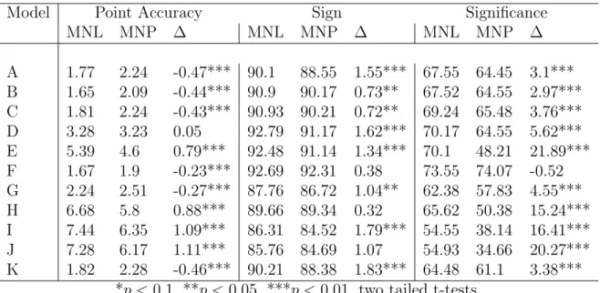
Table 6: Mean Evaluative Measures for MNL and MNP, Britain 1987 Model.
Model Point Accuracy Sign Significance
MNL MNP ∆ MNL MNP ∆ MNL MNP ∆
A 1.77 2.24 -0.47*** 90.1 88.55 1.55*** 67.55 64.45 3.1*** B 1.65 2.09 -0.44*** 90.9 90.17 0.73** 67.52 64.55 2.97*** C 1.81 2.24 -0.43*** 90.93 90.21 0.72** 69.24 65.48 3.76*** D 3.28 3.23 0.05 92.79 91.17 1.62*** 70.17 64.55 5.62*** E 5.39 4.6 0.79*** 92.48 91.14 1.34*** 70.1 48.21 21.89*** F 1.67 1.9 -0.23*** 92.69 92.31 0.38 73.55 74.07 -0.52 G 2.24 2.51 -0.27*** 87.76 86.72 1.04** 62.38 57.83 4.55*** H 6.68 5.8 0.88*** 89.66 89.34 0.32 65.62 50.38 15.24*** I 7.44 6.35 1.09*** 86.31 84.52 1.79*** 54.55 38.14 16.41*** J 7.28 6.17 1.11*** 85.76 84.69 1.07 54.93 34.66 20.27*** K 1.82 2.28 -0.46*** 90.21 88.38 1.83*** 64.48 61.1 3.38***
*p <0.1, **p < 0.05, ***p <0.01, two tailed t-tests.
The simplest way to interpret the results is to determine when one multinomial model
Table 7: Mean Evaluative Measures for MNL and MNP, Britain 1987 Model with Strategic Voting.
Model Point Accuracy Sign Significance
MNL MNP ∆ MNL MNP ∆ MNL MNP ∆
A 1.89 2.33 -0.44*** 89.76 89 0.76** 63.83 60.9 2.93*** B 2.06 2.61 -0.55*** 88.24 87.83 0.41 63.31 60.66 2.65*** C 1.95 2.45 -0.50*** 88.93 88 0.93** 65.76 62.38 3.38*** D 2.04 2.42 -0.38*** 89.76 88.97 0.79** 68.03 65.17 2.86*** E 2.38 2.69 -0.31*** 90.52 89.69 0.83** 69.07 65.76 3.31*** F 1.74 2.02 -0.28*** 91.48 90.17 1.31*** 71.41 70.66 0.75* G 2.12 2.72 -0.60*** 86.83 85.03 1.80*** 58.21 54.03 4.18*** H 3.41 4.41 -1.00*** 86.83 86.14 0.69** 64.97 61.93 3.04*** I 4.04 5.65 -1.61*** 83.55 81.93 1.62*** 54.97 48.55 6.42*** J 4.05 5.64 -1.59*** 82.66 81.52 1.14 55.14 50.55 4.59*** K 2.04 2.61 -0.57*** 87.93 86.83 1.10*** 60.97 58.21 2.76***
*p <0.1, **p < 0.05, ***p <0.01, two tailed t-tests.
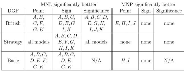
way. The wins for each model are summarized in table 9. It is immediately clear that
MNL has a whole lot more wins than MNP.
For the British models, MNL provides more accurate point estimates for models A,
B, C, F, G, and most importantly K. MNP is more accurate for models E, H, I,
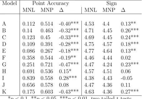
and J. Model D is indeterminate. For the basic models, MNP returns more accurate
point estimates for models H (marginally so), I, and J. Models D and E side with
MNL here. In regards to the sign predictions, MNL predicts the correct sign of the
coefficients for the British models more often than MNP for every correlation structure,
and significantly so for every model except F, H, and J. The basic results for correct
signs are nearly identical, except MNP wins model I, insignificantly. Finally, for the
British models, MNL returns the correct significance levels more often than MNP for
every model except F. For the strategic British models, MNL always outperforms MNP
for all three measures.
Model K contains the “natural” variance-covariance structure from the residuals
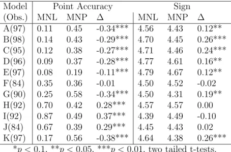
Table 8: Mean Evaluative Measures for MNL and MNP, Basic Model.
Model Point Accuracy Sign
MNL MNP ∆ MNL MNP ∆
A 0.112 0.514 -0.40*** 4.53 4.4 0.13** B 0.14 0.463 -0.32*** 4.71 4.45 0.26*** C 0.123 0.45 -0.33*** 4.69 4.45 0.24*** D 0.109 0.391 -0.28*** 4.75 4.57 0.18*** E 0.086 0.267 -0.18*** 4.77 4.64 0.13** F 0.358 0.544 -0.19** 4.46 4.44 0.02 G 0.251 0.721 -0.47*** 4.47 4.24 0.23*** H 0.691 0.536 0.15* 4.57 4.51 0.06 I 0.839 0.558 0.28*** 4.38 4.43 -0.05
J 0.656 0.578 0.08 4.47 4.36 0.11
K 0.175 0.603 -0.43*** 4.63 4.36 0.27*** *p <0.1, **p < 0.05, ***p <0.01, two tailed t-tests.
situation. MNL outperforms MNP at a highly significant level for all three measures of
model K in the British, basic, and strategic models. This fact suggests that MNL is
far and away a better option than MNP for researchers of the British election. But in
this regard I am only confirming the results of Quinn, Martin, and Whitford (1999) who
suggest that MNL is theoretically more appropriate for Britain and show it empirically.
The results not only confirm what has already been shown for the case of Britain
in 1987, but they demonstrate something about the performance of MNL and MNP in
Table 9: Summary of the Results.
MNL significantly bettter MNP significantly better DGP Point Sign Significance Point Sign Significance
A, B, A, B, C, A, B, C, D,
British C, F, D, E, G E, G, H, E, H, I, J none none
G, K I, K I, J, K
A, B, C, D,
Strategy all models E, F, G, all models none none none
H, I, K
A, B, C, A, B, C,
Basic D, E, F, D, E, N/A H, I none N/A
G, K G, K
accurate point estimates in the British case, and model D which was indeterminate:
χE =
1 . .
.75 1 .
.75 .75 1
, χH =
1 . .
0 1 .
.50 .80 1
,
χI =
1 . .
0 1 .
−.50 .80 1
, χJ =
1 . .
−.20 1 .
−.50 .80 1
,
χD =
1 . .
.50 1 .
.50 .50 1
. (54)
In each of these models, more than one pair of choices are correlated at a level of
magnitude greater than or equal to .5. One pair of choices correlated this highly is not
good enough, as demonstrated by models F and G, in which one pair of choices are
correlated with magnitude .8 but all other pairs are independent. Furthermore, more
than one pair of choices correlated at a magnitude less than .5 is not good enough for