main.pdf

40%—and the use of local, rather than global, modeling to differentiate astrophysical signal from

various forms of radio contaminants. Our algorithm also makes frequent use of robust Chauvenet

rejection (RCR), a new outlier rejection algorithm. RCR is capable of resolving both accurate and

precise mu and sigma values for distributions containing as high as 85% contaminated data, making it

particularly advantageous for removing radio contamination. Together, these techniques produce allow

our image processing software to produce contaminant-cleaned and photometrically viable images for

professional and amateur use.

Fig. 1.—Green Bank Observatory 20-meter diameter radio tele-scope. (Photo credit: GBO)

1.

INTRODUCTION

Skynet is a network of 24 robotic and optical telescopes

scattered across four continents that brings students,

ed-ucators, and professionals access to high-fidelity

astron-omy equipment through a common web-based interface.

Since conceived in 2005, the network has collected over

50,000 users and taken over 15-million images.

Conse-quently, Skynet contributes to diverse research projects,

spanning between work on gamma-ray bursts (Reichart

et al. 2005, Haislip et al. 2006, Dai et al. 2007, Updike

et al. 2008, Nysewander et al. 2009, Cenko et al. 2011,

Cano et al. 2011, Bufano et al. 2012, Jin et al. 2013,

Morgan et al. 2014, Martin-Carrillo et al. 2014, Friis et

al. 2015, De Pasquale et al. 2016, Bardho et al. 2016,

*_{The author would like to acknowledge the significant}

collab-oration with his adviser Dr. Daniel Reichart, along with the cur-rent and former students and software engineers in the Skynet group, specifically Dylan Dutton, Michael Maples, and Travis Berger.

Melandri et al. 2017), variable stars (Layden et al. 2010,

Gvaramadze et al. 2012, Wehrung et al. 2013,

Mirosh-nichenko et al. 2014, Abbas et al. 2015, Khokhlov et al.

2017, 2018), pulsating white dwarfs (Thompson et al.

2010, Barlow et al. 2010, 2011, 2013, 2017, Reed et al.

2012, Bourdreaux et al. 2017, Hutchens et al. 2017),

su-pernovae (Foley et al. 2010, 2012, 2013, Pignata et al.

2011, Valenti et al. 2011, 2014, Pastorello et al. 2013,

Milisavljevic et al. 2013, Maund et al. 2013, Fraser et al.

2013, Stritzinger et al. 2014, Inserra et al. 2014, Takats et

al. 2014, 2015, 2016, Dall’Ora et al. 2014, Folatelli et al.

2014, Barbarino et al. 2015, de Jaeger et al. 2016,

Gutier-rez et al. 2016, Tartaglia et al. 2017, 2018, Prentice et al.

2017), near-earth objects (Brozovic et al. 2011, Pravec et

al. 2014), and even recently the detection of gravitational

wave sources (Abbott et al. 2017a, 2017b, Valenti et al.

2017, Yang et al. 2017).

As part of the American Recovery and Reinvestment

Act of 2009 and in collaboration with Green Bank

Obser-vatory (GBO), Skynet acquired its first radio telescope

from GBO: the 20-meter diameter single-dish radio

tele-scope (Figure 1). After updating of the teletele-scope’s

hard-ware in 2010 and integrating the data acquisition

soft-ware into Skynet, the telescope is now operable by

ed-ucators, students, and professionals through the Skynet

web-interface

_.

In addition to data acquisition, Skynet also offers

in-house processing for images.

While professional

im-age processing procedures are well-established for optical

telescopes, the same is not true for radio telescopes. As

such, Skynet sought to develop equally reliable and

pow-erful processing capabilities for data collected by the new

radio telescope. The two primary challenges to

build-ing such a processbuild-ing pipeline for radio images are (1)

developing the ability to extract radio contaminants in

a user-defined, yet statistically meaningful way, and (2)

providing a means to map radio data to a pixel based

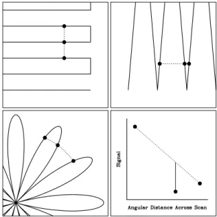
Fig. 2.—Mapping patterns. Left:Raster.Middle: Nodding.Right: Daisy.

age without loosing the resolution capabilities of the

tele-scope. This paper aims to update and validate Skynet’s

preliminary solutions to addressing these two challenges

(Berger 2015) as well as to introduce additional

function-ality and robustness to the processing suite for further

contaminant reduction and scientific use.

1.1.

Radio Data Acquisition and Analysis Techniques

Radio telescopes differ from optical telescopes in two

primary ways: (1) given the low energy of the photons,

the receiver has extremely low resolution and effectively

acts as a single pixel would for a optical CCD. (2) As

a consequence of the low-resolution receiver, it becomes

extremely inefficient and financially nonviable to map an

image pixel by pixel. Instead, radio observations are

col-lected as a sparse grid of single pixel measurements which

later are interpolated to form a final image. The

meth-ods through which these grids are collected are described

below.

1.1.1.

Mapping Patterns

Because radio telescopes operate using a single-pixel

camera receiver, there are two common procedures used

to collect the radio data. First is the point-and-shoot

method, where the telescope slews point-to-point on a

predetermined mapping grid, stopping to integrate at

each predetermined location to produce a flux value. The

point-and-shoot procedure requires frequent acceleration

and deceleration of the telescope—known to cause

sub-stantial wear on the telescope mount. The alternative

method that Skynet has chosen to employ is an on-the-fly

mapping technique where the telescope receiver

contin-ues to integrate as the telescope moves. This minimizes

the amount of strain experienced by the telescope to start

and stop its motion, while also providing greater

flexi-bility for different mapping patterns and a user defined

sampling rate (our default is 0.2 beamwidths).

Specifi-cally, through on-the-fly mapping, the 20-meter telescope

is capable of collecting data in three standard patterns

(Figure 2).

•

Rasters mapping patterns most closely resemble

the rectangular grid utilized by the point-and-shoot

method. Here the telescope maintains either a

con-stant right ascension or declination while sampling

at a constant interval in the alternative coordinate

to produce a single scan. These scans are produced

at predetermined intervals across the field of view

to build a survey of individual scans which together

form the raster mapping pattern.

•

Noddings are mapping patterns that utilize the

rotation of the earth to minimize the amount of

impulse experienced by the telescope.

Popular

for meridian-transit telescopes, the pattern slews

the telescope parallel to the elevation coordinate

thereby utilizing the rotating of the earth to cover

the field of view.

•

Daisy mapping patterns are the most complex

pattern, but also the pattern that puts the least

amount of strain on the telescope. By slowly

accel-erating and decelaccel-erating the telescope around the

source of interest, the telescope never has an abrupt

halt to transition its orientation and collect a new

scan. Instead the telescope smoothly transitions

from one scan into the next. Another advantage

of the daisy pattern is that it can be configured

to collect an arbitrarily large number of scans or

’pedals’ to cross over the source.

Given the variety of mapping patterns, we made it a

requirement of our algorithm to be independent of the

mapping structure of the observation. So long as gaps

between scans do not exceed the Nyquist sampling rate

(≈

0

.

4 beamwidths), all information can theoretically be

recovered.

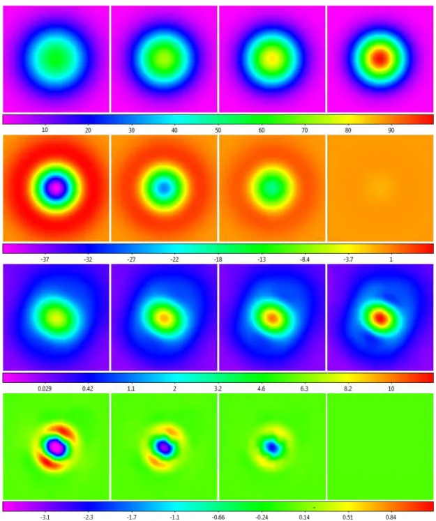
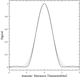
Fig. 3.—First Row: Simulated Gaussian point source sampled on a 1/5-beamwidth grid signal modeled using, from left to right: 1-beamwidth weighted averaging, 2/3-beamwidth weighted averaging, 1/2-beamwidth weighted averaging, and weighted modeling, as described in§2.6.Second Row:Residual error of each technique. Third Row: Cassiopeia A observed with one of the 20-meter’s L-band unfocused linear polarization channels using a 1/5-beamwidth raster. Weighted averaging fails to recover the telescope’s unfocused beam pattern, which is structured. Fourth Row:Difference between each of these techniques and weighted modeling. Square-root and squared scalings are used in the third and fourth rows to emphasize fainter structure (units are dimensionless, with one corresponding to the noise diode; see§2.1.)

So long as the model is sufficiently flexible to model the

source and there is sufficient data to constrain, if not

over-constrain the model, the signal can be recoverable

at any location without blurring. The approach is

out-lined in

§2.6 which demonstrates its ability to resolve

simulated data with less that 1% error near the center of

the beam pattern.

In addition to our decision to model, rather than

av-erage, data, we have also constructed our algorithm to

do all contaminant cleaning before surface modeling—

whereas regridding techniques require cleaning to be

done after signal modeling to accommodate techniques

like frequency clipping within a 2D fourier transform.

1.3.

Contamination Types

Fig. 4.—Weighted modeling of 20-meter data from the third row of Figure 3, at two representative points. Modeled surfaces span two beamwidths, but are most strongly weighted to fit the data over only the central, typically, 1/3 – 2/3 beamwidths, as described in§2.6. Only the central point (red) is retained.

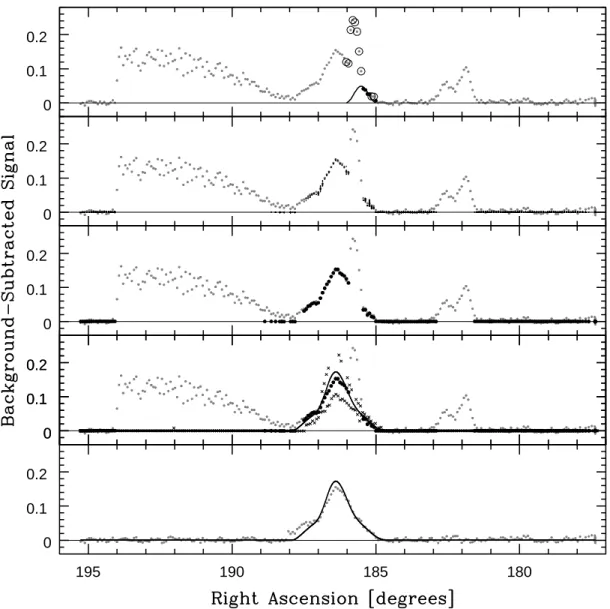
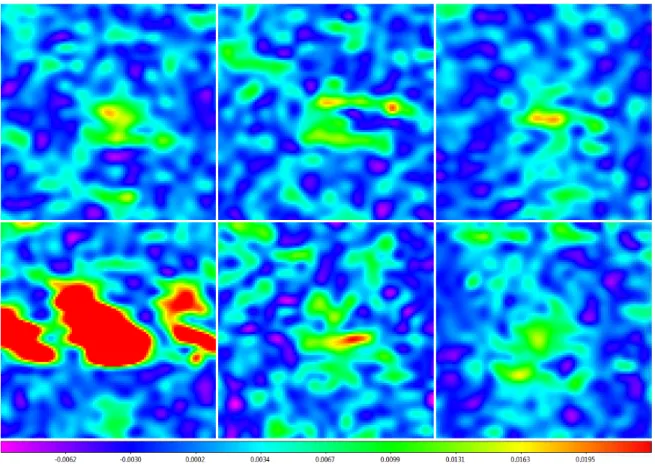
Fig. 5.—Raw map of Virgo A, 3C 270, and 3C 273—top, middle right, and bottom, respectively—acquired with a 1/10-beamwidth raster from the 20-meter in L band. The asymmetric beam pattern characterized in Figure 3 is partially corrected because the left and right channels have been combined prior to surface modeling. Lo-cally modeled surface (§1.2, see§2.6) has been applied for visualiza-tion only. Major signal contaminants (§1.3) are present throughout the image: En-route drift is seen as the the low-level variations along the horizontal scans, RFI is visible during the scan that passes through 3C 273 and near Virgo A, and elevation-dependent signal becomes pronounced toward the upper right (≈11◦ above the horizon).

have collectively been referred to as the ”scanning effect”.

These include 1/f noise, pink noise, and environmental

variations in the atmosphere or spillover when the

tele-scope points too close to the ground. These low-level

contaminants are most noticeable scan-to-scan and can

be made to vary over longer or shorter angular distances

by moving the telescope faster or slower.

Sofue & Reich (1979) attempt to eliminate en-route

drift by first isolating the en-route drift through unsharp

masking and then modeling the drift using a second-order

polynomial while using sigma clipping to extract only the

small-scale structure from the scan. The faults in these

procedures, however, are (1) that low-order polynomials

may be inadaquate when modeling en-route drift over

large angular scales, (2) unmasking requires the

blur-ring of data, a disadvantage we are seeking to avoid, and

Fig. 6.—Green Bank Observatory 40-foot diameter radio tele-scope. (Photo credit: GBO)

(3) sigma clipping is a non-robust outlier detection

algo-rithm.

Emerson & Grave fourier transform the data and mask

near-zero frequencies that contain the en-rout drift.

Ide-ally, this procedure is conducted when there are two

maps with scans in orthogonal directions each

trans-formed such that the real spacial frequencies can be

re-tained. While this method does not assume that en-route

drift can be modeled with a simple low-order function, it

does unfortunately require that data be processed on a

grid, and for best effects, requires that two orthonormal

surveys be collected for the most accurate processing.

Furthermore, this technique is not generalizable for

non-rectangular mapping patterns, eliminating the possibility

to remove the drift from daisies and noddings.

contam-Fig. 7.—Flowchart of our algorithm for contaminant-cleaning and mapping small-scale structures. Blue boxes represent the internal algorithms, green ovals are the I/O of the corresponding algorithms, particularly the raw data, noise models, and maps. Red ovals are user-chosen parameters useful for isolating wanted and unwanted structures as well as final mapping.

inant. Given that temporarily local RFI does not exceed

a beamwidth in scale, and moreover does not extend into

multiple scans, it is possible to model data over the

char-acteristic beamwidth scale in a 2D space and isolate the

contaminant.

Elevation dependent signal occurs when the telescope

slews close enough to the ground that terrestrial signal

begins to spill into the antenna. Often this signal gets

disguised in en-route drift, but it becomes apparent at

high elevations.

Despite the differing modes of contaminant production,

our algorithm models all of these contaminants the same

way.

By locally modeling the data with second-order

polynomials, and using a robust form of outlier rejection

to eliminate inaccurate local model values, our algorithm

is capable of constructing a global model for each data

point free of contamination.

1.4.

Robust Chauvenet Rejection

Sigma clipping is one of the simplest forms of outlier

rejection; however, it is also one of the crudest. To use

sigma clipping, scientists have the flexibility to

deter-mine how many sigma to consider characteristic of a

distribution before excising them from the data set—a

highly non-statistical procedure. One of the more

pop-ular attempts to remove this user-dependent ambiguity

is Chauvenet’s rejection, which is sigma clipping plus a

reasonable rejection criteria:

N P

(

>

|z|) = 0

.

5

,

(1)

18400 18450 18500 0.4

0.5 0.6 0.7

Fig. 8.—40-foot gain calibration data, with the noise diode first on and then off, and best-fit model. Circled points have been robust-Chauvenet rejected, including data taken during the transi-tions from off to on and on to off, and RFI-contaminated data. The background level increased during the calibration, but our model accounts for this: Simply averaging each level, instead of modeling each level with a line, would have underestimated the result.

7.24 7.25 7.26 7.27 7.28 7.29

16.2 16.4 16.6 16.8 17 -0.005

0 0.005

Fig. 9.—Point-to-point noise measurement technique.Top: The technique used for gain-calibrated 20-meter data—circled points were robust-Chauvenet rejected. Bottom:Deviations. Mean and standard deviations are measured from the non-rejected points, for each scan.

contaminated distributions. We have developed a new

form of outlier rejection called robust Chauvenet

rejec-tion (Maples et. al. 2017) which resolves this ambiguity

through the use of more robust measures of central

ten-dency including mode, median, and the 68%-percentile

deviation in an iterative fashion to remove the most

ex-treme outliers before using more precise metrics such as

the mean. This technique is used frequently throughout

this paper, serving as a field-test to the integrity of the

algorithm.

2.

SOFTWARE

0 50 100 150 200 0.004

0.005 0.006 0.007

Fig. 10.—Corrected 1D noise measurements vs. scan number for a 20-meter observation, and best-fit model. Only two points met the robust Chauvenet rejection criterion, and then only barely, which is not unusual given that intra-scan outliers have already been rejected (Figure 9). The 1D noise level increased by ≈20% over the course of this observation.

In this section we outline the set of algorithms

cre-ated to contaminant clean and map small-scale

astro-physical structure (Figure 7). In

§2.1 we calibrate the

telescope against often small, variations in gain. In

§2.2

we measure the point-to-point variation in signal which

can be used to understand the characteristic noise of the

data along a particular scan. In

§2.3 we separate

small-scale astronomical structure from both long- and

short-duration RFI (including en-route drift, elevation signal,

and large scale structure).

In

§2.4, we cross-correlate

our scans to account for any time delay effect between

the coordinate and signal device. In

§2.5 we measure

the noise differences between scans as a metric to further

isolate instances of short-duration RFI from data points

near the signal. In

§2.6 we detail our surface modeling

algorithm’s ability to interpolates data without blurring

it beyond the instrument’s resolution. Finally, in

§2.7 we

outline the various image data products produced for the

user.

2.1.

Gain Calibration

Signal measurements in radio telescopes are calibrated

against a noise diode. Ideally this is done when the

tele-scope tracks the same point across the sky to minimize

the amount of interference in the measurements. These

measurements, however, are imperfect and are

suscepti-ble to extraneous noise as well as sensitivity to the diode

transitioning between on and off. Consequently, we use

RCR to reject the anomalous data and then we fit a line

for both the diode being on and the diode being off. The

difference between these two lines, ∆, is what is used to

calibrate the data (Figure 8).

Given that the 40-foot telescope

_{and the 20-meter}

telescope do not vary substantially over the time scale

3 _{Skynet also makes use of data collected by the 40-foot}

L and X bands, and consequently, we recommend larger background-subtraction scales here. This compo-nent was significant in L band prior to 8/1/14, as can be seen in the third row of Figure 3, as well as in Figure 5. Post 8/1/14, it was significantly re-duced, but not altogether eliminated. This component corresponds to ap-proximately 2% – 3% and 4% – 5% of the integrated beam pattern in L and X band, respectively. If this is not a concern, these minimum recom-mended 1D background-subtraction scales can be lowered to 3 and 4 the-oretical beamwidths, respectively.

of the observation, we choose to calibrate only at the

be-ginning and end of the observation. We then allow the

user to choose between using the calibration at the

be-ginning ∆

, end ∆

, or a linear interpolation between

the two:

∆(

t

) = ∆

+ (∆

−

∆

)

t

−

t

t

−

t

.

(2)

We calibrate each polarization channel individually and

the user can choose to continue using either channel or a

composite channel that sums the fluxes of both.

2.2.

1-D Noise Measurement

Here we measure the standard deviation of data on the

most fundamental object type, the scan. For each data

point within the scan, we fit a line to the two nearest

non-rejected data points, and measure the deviation of

the central point off of that line (Figure 9). Once a

col-lection of these deviations are collected, we use RCR to

extract the average deviation value, which tends towards

zero, and its standard deviation which we then use as

the noise model for the scan. We also allow for the noise

value to change over time, so once all individual scan’s

noise model has been constructed, we fit a line to their

standard deviations using RCR to model the change in

noise over time (Figure 10). This prevents scans that

have excessive RFI from producing an

uncharacteristi-cally high noise value for a temporally anomalous set of

events. The final value is the noise model for each signal

measurement within that scan.

2.3.

Background Subtraction

The majority of contaminants in radio data occur at

the background level. Flux measurements can be biased

8 10 12 14 16

7.6 7.65 7.7

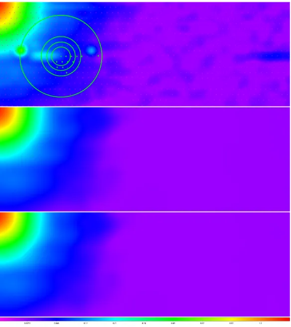
Fig. 11.— Top: A local background model applied in the for-ward direction and anchored to an arbitrary point from Figure 5, near 3C 270. Circled points indicate data that are within one background-subtraction scale length, but that still remain above the model. Middle: Forward- and backward-directed local back-ground models, anchored to every point in the scan. Bottom: Global background model, constructed as a non-linear combina-tion of lowest local background models.

by the dish pointing too close to the horizon causing the

earth’s own radio emission to interlace with the

astro-physical data. Features of long-duration RFI can

cor-rupt a broad region of data points between one or more

scans. Atmospheric variation and large-scale

astrophys-ical structure can overlap with the small-scale structure

source. To distinguish these deviant features from the

small-scale sources, traditional algorithms fit lines

be-tween each point to every other point, and maintain only

those that have all data between them above the line.

This results in a global background model that falls

en-tirely beneath the data, underestimating the background

contamination given its extreme sensitivity to radio noise

in the negative direction (Figure 11).

To distinguish between astrophysical sources and

back-ground contaminants, our algorithm instead models data

locally over a user-defined scale. At each point, the

al-gorithm collects all data within the user-defined scale

and in the same scan. It then fits a quadratic regression

model to the data (as opposed to linear which is often

too inflexible to model contaminants), and calculates the

total deviation of the collected data from the model. If

the deviation exceeds the characteristic noise of the scan

(as determined in

§2.2), the most deviant point off of the

model is removed, and the model is refit

. This cycle is

4 _{To ensure the model does not underestimate the background}

7.6 7.65 7.7 7.6 7.65 7.7

8 10 12 14 16

7.6 7.65 7.7

Fig. 12.—Top:A preliminary local background model, anchored to the same point as in Figure 11. Circled points have been itera-tively rejected as too high, given the modeled noise level (§2.2); the larger points were not rejected. Middle: Final local background models once the original point is unanchored and is free to be re-jected. Bottom:Global background model, constructed from the final local background models.

iterated through until the total deviation off of the model

is less than the scatter within the original data.

_These

models will be fit through each data point, and once the

model falls within the scatter of the scan, the resulting

values of the model at each of the data points’ location

will be saved.

Once complete, each datum will contain a distribution

of local-model values from these background fits, from

which RCR can extract an accurate and precise

global-model for the background flux at that point. We use

weights that strengthen models that are produced near

the center of the data, as their regression is more likely

to be a more appropriate fit than unbound tales:

w

=

P

j

N

1 +

σi

+

δ

κi

,

(3)

where

P

j

N

is the number of non-rejected dumps that

contributed to the

i

th local background model,

w

is the

weight of the

j

th point from the

i

th local background

model,

x

is the angular distance of this point along the

scan,

µ

is the dump-weighted mean angular distance of

value. At this point, we unanchor this point and allow the model to be refit and iteratively allow points back in to ensure there was not an overrejection of data. This allows the global model to fit within the noise level of the data rather than under it (Figure 12)

5_{If the algorithm continues to reject data such that there is no}

longer sufficient data to model a quadratic regression, the algorithm will attempt a linear fit and repeat this procedure.

-2 0 2 -1 0 1

Fig. 13.—Gaussian random noise background-subtracted (top) and residuals (bottom) vs.W, the sum of the weights of the non-rejected local background models that determine the global back-ground model at each point, for 1/10- and 1/5-beamwidth rasters, and for 1-, 3-, 6-, 12-, and 24-beamwidth background-subtraction scales (background-subtraction scale times sampling density of the data sets increases from left to right). The RMS of the data varies with W, but not with background-subtraction scale or sampling density independently. Curves are 1-, 2-, and 3-σmodel noise en-velopes that have been fitted to all of these data simultaneously (Equations 6 and 7).

all of the non-rejected points from the

i

th local

back-ground model,

σ

is the dump-weighted standard

devia-tion of these values,

κ

is analogous to standard

devia-tion, and is related to these values’ kurtosis:

κ

=

" P

j

N

(

x

−

µ

)

P

j

N

#

,

(4)

and

δ

is zero for linear local background models and one

for quadratic local background models (analogous terms

can be added for higher-order local background models).

Once calculated, the the user has a global background

model which can be subtracted off of the original data

to remove long-duration RFI, elevation dependence,

en-route drift, and underlying large-scale structure.

2.3.1.

Background Subtraction Verification

To test the validity of this procedure, we designed a

simulated data set that layers increasingly prominent and

complex containment types.

_{The first layer includes a}

standard gaussian noise model across the image. We

ap-ply our background subtraction procedure using 6-,

12-, and 24-beamwidth background scale and evaluate its

Fig. 14.—Left:Factor by which background subtraction reduces en-route drift (red), long-duration RFI (green), large-scale astronomical signal (blue), elevation-dependent signal (purple), and short-duration RFI (black) in our simulated data, for background subtraction scales of 3, 6, 12, and 24 beamwidths (dashed curves). Factor by which background and RFI subtraction (see§2.5) reduce these contaminants (solid curves). Right: Fraction of the noise level to which these contaminants are reduced. If nothing is plotted, the contaminant is completely eliminated on this scale. For these measurements, each contaminant was simulated separately, and in the absence of sources.

performance by measuring the residual off of the

uncon-taminated values (Figures A.1 and A.2). We find that

the background subtracted data are neither biased high

or low and the noise level is nearly identical to that of

the original data. Furthermore, the RMS of the residuals

is much less than the original data. These quantities are

determined by the number of local models to the point

j

’s

global models, as well as their collective weights. For

ex-ample, for smaller background scales or closer to the edge

of the scan where fewer data are collected, the greater the

residual RMS values. These residuals are plotted against

the summed weight,

W

, of all local models in Figure 13

where

W

=

X

i

w

.

(5)

We supplement this data using 1- and 3-beamwidth

background scales and find that the noise level of the

background-subtracted data is well-modeled by:

σ

≈

0

.

979

−

0

.

275

e

(6)

and that the RMS of the residuals is well-modeled by:

σ

≈

0

.

131 + 0

.

334

e

,

(7)

of

W

suggesting that no additional variability is being

included through the routine itself.

In conclusion, background subtraction errors in the

ab-sence of small- or large-scale data by a factor as high as

≈

47% of the original noise for small

W

values to as low

as

≈

13% for large values of

W

. Furthermore, these are

random errors biasing the data equally in the positive

and negative directions, reducing the noise of the data

by

≈

30% for very small values of

W

to only

≈

2% for

large values of

W

.

Next we add simulated gaussian point sources to our

image as well as short duration RFI (Figure A.3). We

again background subtract with scales of 6-, 12-, and

24- beamwidths, and extract their residuals (Figure

A.4). We find three underlying causes of the residuals.

The first is an underestimation directly underneath the

source, however it is independent of the brightness of the

source. The bias level is best defined by

peak bias level

≈ −

(0

.

5

−

1)

×

noise level

background subtraction scale 6 beamwidths

.

(8)

which is at a sufficiently low level that it can be ignored.

Furthermore, when the sources are replaced with cosine

functions with less winged tails, the factor decreases by a

factor between 2 and 3. These systematic biases are

fur-ther corrected by our RFI-subtraction algorithm (§2.5)

in regions near the sources.

The second bias is attributed to sources that are close

in proximity as collectively they can exceed the length of

the original background subtraction scale. These effects

are best mitigated by use of larger background-scales

such as 12- and 24-beamwidths.

The final bias occurs when a source lay within 1- to

2-beamwidths of the edge of the survey—an area where

the background model no longer has sufficient data to

constrain its regression. This is a known deficiency in

our algorithm, but it is local and easy to define allowing

us to give the user the option to clip these data before

surface-modeling if desired.

Next in our simulated image we include en-route drift

and long-duration RFI (Figure A.5). Like the gaussian

noise and the point sources, we model these data

us-ing a 6-, 12-, and 24-beamwidth scale and measure the

residuals (Figure A.6).

We find that the background

subtraction routine is effective at reducing the effects

of the contaminants given that the background-scale is

sufficiently below the scale of the large-scale structure

(12-beamwidths in this simulation). We find that

en-route drift and long-duration RFI are reduced by

fac-tors of

≈3 and

≈5, to

≈96% of and

≈53 times the

noise level, respectively, when background-subtracted on

double this scale (24-beamwidths); by factors of

≈63

and

≈630, to

≈5% and

≈39% of the noise level,

re-spectively, when background-subtracted on half of this

scale (6-beamwidths); and by even greater factors when

background-subtracted on even smaller scales (see

Fig-ure 14). These gains are significantly furthered by our

RFI-subtraction algorithm.

Lastly we include 2D large-scale structure and find that

the results are closely paralleled to that of long-duration

RFI and en-route drift (Figure A.7). We find that

large-scale astronomical and elevation-dependent signal is

re-duced by factors of

≈26 and

≈670, to

≈3 times and

≈18% of the noise level, respectively, when

background-subtracted on the scale of the map (24 beamwidths); by

factors of

≈830 and

≈3400, to

≈11% and

≈4% of the

noise level, respectively, when background-subtracted on

the 6-beamwidth scale; and by even greater factors when

background-subtracted on even smaller scales (Figure

A.8).

2.3.2.

20-Meter and 40-Foot Data

After verifying functionality of background subtraction

on simulated data, we proceed to test its functionality on

real data from the 20-meter and 40-foot telescopes. We

demonstrate its function on a 20-meter L-band raster of

Virgo using both small and large background-subtraction

scales (Figure 15), two heavily contaminated maps of

An-dromeda (Figure 16), a daisy map of 3C 84 taken with

the 20-meter in X Band to demonstrate its application

on non-rectangular mapping patterns (Figure 17), and

finally two nodding maps of the sun using the 40-foot

(Figure 18).

2.4.

Time-Delay Correction

In the case of the 20-meter telescope, the signal is

in-tegrated over a user-defined time, and coordinate

infor-mation is recorded at the midpoint of this integration

time. However, with the 40-foot, signal is run through an

RC filter, with a user-defined time constant, typically 0.1

seconds, but signal and coordinate values are sampled

si-multaneously, resulting in an effective delay between the

two due to the time constant (Figure 20). This results in

alternating coordinate errors in alternating scans. Even

with the 20-meter, the same can happen if the signal and

coordinates computers’ clocks become unsynchronized.

To correct for this, we cross-correlate adjacent scans.

The position of the maximum value of the

cross-correlation gives the best angular shift between the scans,

and the square root of this value gives a weight. If the

scans intersect a source, the best angular shift is well

defined, and the weight is correspondingly high. If they

intersect only noise, the best angular shift is not well

de-fined and the weight is low. For all adjacent scans we

measure the best angular shift and reject outliers using

RCR and take the mean of the remaining values and

di-vide by the telescopes slew speed to convert to time. We

again perform RCR to eliminate periods of telescope

ac-celeration (Figure 19). We then take the final time and

interpolate the telescope’s coordinate values accordingly.

2.5.

RFI-Subtraction

Once long-duration contamination has been removed

and the individual scans are aligned with one

an-other, the algorithm proceeds to remove remaining

RFI-contaminants.

The procedure involves fitting a

two-dimensional cosine to local data, and, in a manner

sim-ilar to background subtraction, rejecting deviant points

and remodeling the cosine until the total deviation

be-tween data and model falls within the characteristic noise

(§2.5.1) of the survey.

2.5.1.

2-D Noise Model

Fig. 15.—20-meter L-band raster from Figure 15 background-subtracted, with 7- (left; Table 1) and 24- (right) beamwidth scales (the map is 24 beamwidths across). Locally modeled surfaces (§1.2, see§2.6) have been applied for visualization only. Hyperbolic-arcsine scaling is used to emphasize fainter structures.

Fig. 17.— Left: Raw map of 3C 84, acquired with the 20-meter in X band using a 20-petal daisy pattern. Right: Data from the left panel background-subtracted, with a 6-beamwidth scale (Table 1). Locally modeled surfaces (§1.2, see§2.6) have been applied for visualization only.

0.001 0.01 0.1 1 -10

Fig. 19.—Best angular shift between adjacent scans vs. cross-correlation weight for all scans in a 20-meter observation. Many of the low-weight best angular shifts are not well defined, because their corresponding scans are noise-dominated. A few of the high-weight best angular shifts are incorrect, due to RFI contamination (consequently, simply taking the weighted mean of these values would yield a poor result). To eliminate both cases: For each best angular shift, we calculate the probability that it could, by chance alone, be as close as it is to both its preceding and proceeding values,a _{and eliminate all best angular shifts for which this}

proba-bility exceeds one half divided by the best angular shift sample size (e.g., Chauvenet 1863, Maples et al. 2017; squared points). The remaining best angular shifts repeat consistently for at least three consecutive measurements, and consequently are likely due to as-tronomical signal, not noise or RFI contamination. We take the unweighted mean of these values (line), robust-Chauvenet rejecting any remaining outliers (circled points).b

a_{For two, adjacent, best angular shifts, δ}

i and δi+1, it is

not difficult to show that this probability is given by pi,i+1 =

|δi+1−δi| ∆

2−|δi+1−δi| ∆

, where ∆ is the angular length of the

scans. For three, this probability is given by 2pi−1,ipi,i+1. b_{We reject outliers as described in§8 –§10 of Maples et al. 2017,}

using iterative bulk rejection followed by iterative individual rejec-tion (using the mode + broken-line deviarejec-tion technique, followed by the median + 68.3%-value deviation technique, followed by the mean + standard deviation technique), using the smaller of the low and high one-sided deviation measurements. Data are weighted equally, in case any of the remaining high-weight data are still bi-ased by RFI contamination (or by source saturation, as is the case in Figure 18).

as the 2-D noise, and its measurement includes taking

each data point within a scan, identifying the closest

da-tum in the proceeding and preceding scans, fitting a line

to those two datum and then measuring the deviation of

the original point from this line. Once all data deviations

within the scan have been measured, RCR is then used

to remove the most discrepant deviations and to extract

the precise across-scan noise value for that scan. This is

repeated for each scan within the survey. Once all scans

have a characteristic two-dimensional noise value, a line

is fit to these data across the scans on which RCR is

again performed. This prevents scans contaminated by

long-duration RFI to bias the characteristic noise of the

larger survey (Figure 22). When fitting to

uncontami-nated gaussian data, we find this method overestimates

the true noise value by 22.9%. We correct each scan’s

noise value accordingly.

z

(∆

θ

) =

(

f

cos

+

z

if ∆

θ < θ

0

otherwise

,

(9)

where ∆

θ

is the 2D angular distance from the model’s

center,

θ

is a user-defined RFI-subtraction scale, and

f

, the first of the two fitted parameters, normalizes the

function in the first term, and

z

, the other fitted

param-eter, adds a small, local, background value(Figure 23).

This allows us to model a point source almost exactly

when

θ

≈

1 beamwidths, and if

θ

is chosen to be

slightly smaller than the true FWHM of the telescope’s

beam pattern, it can be used to separate astrophysical

signal from marginally sub-beamwidth structures.

This model is centered at each data point, and the

algo-rithm proceeds to calculate the total deviation of all data

from the model. If the deviation exceeds the anticipated

two-dimensional noise value, it then proceeds to reject

the most positive outlier if

f >

0 or the most discrepant

outlier if

f <

0 and refit. The procedure continues on

until the standard deviation of the non-rejected points

is consistent with the noise model. The end product

re-sults in a singular local model, defined only at the

non-rejected points (Figure 25). This procedure is repeated

for all data within the survey, constructing a distribution

of local models for each data point.

Once local models are constructed for each data point,

the algorithm performs RCR on each datum’s local

model distribution to construct the global model value.

RCR’s output produces the RFI-cleaned data points

which will be used for surface modeling (§2.6). All data

that never earned a local model are assumed to be RFI

and are excised from the data set.

In theory, the RFI-subtraction scale need be only

slightly smaller than the FWHM of the beam pattern to

successfully remove contaminants. However, in practice,

the source may be more peaked than the model or

asym-metric. In these cases, a smaller RFI-subtraction scale is

recommended, but the user is cautioned to remain aware

that smaller scales risk high rejection rates of data that is

part of the astrophysical source (Figure 32). We present

recommended RFI-subtraction scales for both the

20-meter and 40-foot telescopes in Table 2.

2.5.3.

RFI-Subtraction Verification

Fig. 20.— Background-subtracted map of Cassiopeia A in L band, acquired with the 20-meter with signal and position computers’ clocks unsychronized, before (left) and after (right) time-delay correction. Locally modeled surfaces (§1.2, see§2.6) have been applied for visualization only. Square-root scaling is used to emphasize fainter structures.

Fig. 21.— Scan-to-scan measurement technique as applied to the three primary mapping techniques. Residuals are measured (bottom right), and mean and standard deviations are measured from the non-rejected points, for each scan.

First we analyze the algorithm’s performance on gaussian

noise with a RFI-subtraction scale of 0.95 beamwidths as

well as a RFI-subtraction scale of 0.5 beamwidths

(Fig-ure B.1). We find that the RFI-subtracted data are not

biased high nor low and the noise level is significantly less

than the original background-subtracted data. We then

TABLE 2

Maximum Recommended 2D RFI-Subtraction Scale for the Telescopes and Receivers of§2, in Theoretical

Beamwidths

Telescope Receiver Scale

Left or Right Left + Right Channel Channel

20-meter L (HI + OH)a 0.8 0.9

20-meter L (HI)b _{0.7 0.8}

20-meter L (OH)b _{0.9 1.1}

20-meter X 0.8 0.8

40-foot L (HI) 0.7 0.7

a_{Before August 1, 2014}

b_{After August 1, 2014}

Fig. 22.— Left: Corrected 2D noise measurements vs. scan number for the 20-meter observation from Figure 10, after background-subtracting on a 6-beamwidth scale, and best-fit model (solid line). Circled points have been robust-Chauvenet rejected. 1D noise model from Figure 10 is included for comparison (dashed line). The 2D noise level is≈28% higher, due to residual 1D structures (e.g., residual en-route drift) post-background subtraction. Right: Same, but with a 24-beamwidth background-subtraction scale. In this case, the 2D noise level is≈46% higher than the 1D noise level, because contaminants are less completely eliminated on longer background-subtraction scales (e.g., Figure 14).

-2 -1 0 1 2

0 0.2 0.4 0.6 0.8 1

Fig. 23.—Local model (Equation 9) withθRF I= 1 beamwidth and z0 = 0 (solid curve), and Airy (dashed curve) and Gaussian

(dotted curve) functions, each with FWHM = 1 beamwidth.

Next we include 1D large-scale structure

contamina-tion in the form of en-route drift and long-duracontamina-tion RFI.

We find that long duration RFI is now reduced by a

factor of

≈

19000 to

≈

1% of the noise level when the

background-scale was 24-beamwidths (Figure B.3). The

signal was further reduced when the background-scale

approached 6-beamwidths. We also find that en-route

drift is reduced by a combined factor of

≈

20 to

≈

16% of

the noise level when background subtracted on the scale

of the map; this factor increases to a factor of

≈

730 or

≈

0

.

4% of the noise level when background-subtracted

on the 6-beamwidth background-subtraction scale. For

reference, the basket-weaving technique of Winkel, Floer

& and Krauss (2012) reduces en-route drift by a factor

of

≈

10 under ideal circumstances.

Finally, we include 2D large-scale structure

contamina-tion through the inclusion of elevacontamina-tion-dependate signal

and background structure (Figure B.4). Away from the

sources, we find that the elevation-dependent signal is

reduced by a combined factor of

≈

2800 or

≈

4% of the

noise level when background subtracted on the scale of

the map (24-beamwidths). The signal is reduced to

im-measurable levels when background subtracted on the

6-beamwidth scale. We find that the astronomical signal

is reduced by a combined factor of

≈

800 to

≈

11% of

the noise level when subtracted on the scale of the map,

and to a factor of

≈

5900 or

≈

2% of the noise level when

background-subtracted with a 6-beamwidth scale.

2.5.4.

RFI-Subtraction on Real Data

After verifying the effectiveness of RFI-subtraction on

simulated data, we proceed to test its functionality on

real data. First we use a wide-field survey with extreme

amounts of RFI-contamination collected by the 40-foot

telescope (Figure 26). The contamination was the result

of a broadband emitter from the Roanoake, VA airport

located 100 miles south of Green Bank. The signal is

linearly polarized appearing in only one of the telescopes

two channels. We find that after RFI-subtraction the

contaminated and uncontaminated channels are nearly

identical.

We also apply our RFI-subtraction procedure to

Fig-ure 16 and FigFig-ure 15 to produce FigFig-ures 27 and 30.

0

0.1

0.2

0

0.1

0.2

0

0.1

0.2

0

0.1

0.2

0

0.1

0.2

195

190

185

180

0

0.1

0.2

Fig. 24.—First:1D cross-section along a scan that simultaneous visualizes a profile of a single 2D local model, centered on an arbitrary point from the left panel of Figure 15, near Virgo A (curve). We have contaminated this scan with three instances of simulated RFI (the original, uncontaminated data are plotted in the fifth panel). Circled points have been iteratively rejected as too high, given the modeled noise level (§2.5.1); the larger, darker points were not rejected. Second: Every local model that intersects this scan, evaluated at each local model’s non-rejected points (smaller, darker points). All simulated RFI has been rejected, being too narrow—as compared to the RFI-subtraction scale (θRF I = 0.9 beamwidths; Table 2)—either along or across the surrounding scans. Third: Global model (larger, darker points), produced via RCR on the distributions of local models at each point. Fourth: 1D cross-section of the 2D surface model (§1.2, see§2.6), constructed from the 2D global model, three scans of which are shown (this scan = larger, darker points; adjoining scans = crosses). Differences between data and model are due primarily to residual en-route drift, which differs from scan to scan. Fifth: The same, but constructed from the original, uncontaminated data, demonstrating the effectiveness of this approach to RFI subtraction.

removed. This is best demonstrated by our constructed

map of Jupiter, a particularly faint radio emitter (Figures

28 and 29), and Barnard’s loop (Figure 33). A similar

appending procedure is available to the user for

sepa-rate fields of view; however, greater care must be

exer-cised to ensure that the data is equally calibrated, and

that the edge of one map is not characterized as an

out-lier compared to the other map given both

background-subtraction and RFI-background-subtraction’s underestimation near

the ends of scans.

Finally, we test RFI-subtraction on a daisy mapping

pattern to verify the functionality on non-rectangular

mapping types (Figure 31).

2.6.

Surface Modeling

computa-Fig. 25.—Top: Zoom-in of the first panel of Figure 24, but in 2D. Purple dots mark observation points. Green contours mark the 0%-, 25%-, 50%-, 75%-, and 100%-of-peak levels of the local model. Green plusses mark observation points within the domain of the local model that were not rejected, for being too high, given the modeled noise level (§2.5.1). Locally modeled surface (§1.2, see§2.6) has been applied for visualization only. Middle: Zoom-in of the fourth panel of Figure 24, in 2D.Bottom:Zoom-in of the fifth panel of Figure 24, in 2D, which is nearly identical, despite not being contaminated with the simulated RFI.

tion time, but given that our data is already contaminant

cleaned there is substantially less computation time

ded-icated to surface modeling than would be required by

previous algorithms.

For each pixel, we fit a flexible surface model to all data

that are within 1-beamwidth, weighting data that are

closest to the pixel highest. We evaluate the model only

at that pixel, so it only needs to fit well here. We have

found using a third-order 2D polynomial is sufficient at

modeling the data without blurring beyond instrument

resolution while also having few enough parameters to

ensure the fit is always well constrained for most

sam-pling densities and mapping patterns:

z

(∆

x,

∆

y

) =

3

X

i=0 3−i

X

j=0

a

(∆

x

)

(∆

y

)

,

(10)

where

z

is the locally modeled signal, ∆

x

and ∆

y

are

angular distances from the central pixel along each

co-ordinate, and

a

are the polynomial coefficients.

At

this pixel, Equation 10 simplifies to

z

(0

,

0) =

a

, which

streamlines the computation. We repeat this process for

all pixels in the image.

We weight the data using a similar model to equation

9 except raised to a power:

w

(∆

θ

) =

_cos

2 beamwidths

if ∆

θ <

1 beamwidth

0

otherwise

,

(11)

where:

α

=

−

log 2

log

cos

4 beamwidths

,

(12)

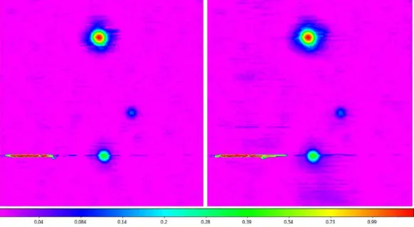
Fig. 26.—Top Left: Background-subtracted mapping of, from right to left, 3C 84, NRAO 1560/1650, 3C 111, 3C 123, 3C 139.1, and 3C 147, as well as fainter sources, acquired with the 40-foot in L band, using a maximum slew speed nodding pattern. The data are heavily contaminated by linearly polarized, broadband RFI, affecting only one of the receiver’s two polarization channels. Top Right: Data from the top-left panel time-delay corrected and RFI-subtracted, with a 0.7-beamwidth scale (Table 2). Bottom Left: Identically processed data from the receiver’s other, relatively uncontaminated polarization channel, for comparison. The RFI-subtraction algorithm is not perfect, but performs very well given the original, extreme level of contamination. Bottom Right: Background-subtracted and time-delay corrected data from both, equally calibrated polarization channels first appended and then jointly RFI-subtracted. Locally modeled surfaces have been applied for visualization (§1.2, see§2.6).

function. This weighting scheme allows for the weight

to approach zero at the

θ

= 1 limit. This ensures no

discontinuities as new data is introduced to the moving

model. For smaller

θ

values, we weight points nearest to

the pixel as most significant to generate a more accurate

fit. However, smaller

θ

values also reduce the number

of points to constrain the model risking the potential

in-crease in noise and a less precisely modeled fit. We have

found that Equation 10, is sufficiently flexible to

repro-duce most all diffraction-limited structures, to

>

99%

accuracy, if

θ

≤

1

/

3 beamwidths. That said, unless one

is trying to visualize narrow contaminants like RFI or

en-route drift, there is no advantage to surface modeling

using

θ

<

1

/

3 beamwidths. Furthermore, for increasing

values of

θ

beyond 1

/

3, image accuracy is reduced only

marginally, while precision grows significantly more

pre-cise. For example,

θ

= 1

/

2, 2

/

3, and 1 beamwidths

re-sult in only

≈2%,

≈4%, and

≈6% underestimates at the

source’s peak, respectively, and these underestimates are

almost perfectly compensated by overestimates at the

source’s base. Finally,

θ

must be sufficiently large to

encompass enough data to constrain equation 10.

To

ensure this requirement, our algorithm enforces that

θ

=

max

θ

, min

₄

3

×

θ

,

1 beamwidth

,

(13)

where

θ

is the largest spacing between the pixel and

the nearest local points as discussed in Figure 37. For

computational efficiency and modeling accuracy, we

mea-sure the value of

θ

for each data point and interpolate

afore-Fig. 27.—Background-subtracted and time-delay corrected 40-foot noddings of Andromeda from Figure 16 (1) separately RFI-subtracted (left and middle), and (2) appended and then jointly RFI-subtracted (right), with a 0.7-beamwidth scale (Table 2). These maps are relatively free of RFI; as such, the appended map is nearly identical to what one gets from averaging the first two maps, but is nearly twice as efficient to produce, computationally (see below). Locally modeled surfaces have been applied for visualization, with a minimum weighting scale of 1/3 beamwidths (§1.2, see§2.6).

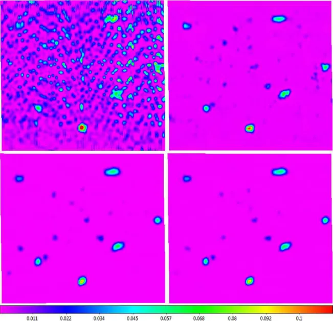
Fig. 28.—Six background-subtracted mappings of Jupiter, acquired with the 20-meter in L band, using 1/5-beamwidth rasters. Jupiter is only marginally detected in each, except for the fourth, which is significantly contaminated by RFI. Locally modeled surfaces (§1.2, see

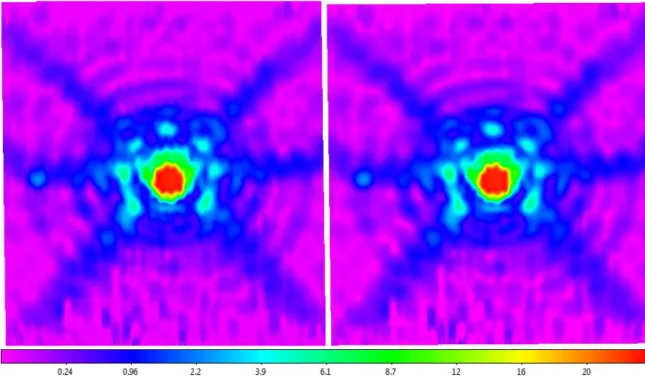
Fig. 29.—Top Row:The six background-subtracted mappings of Jupiter from Figure 28 appended and jointly RFI-subtracted, with 0.9-(left), 0.1- (middle), and≈0- (right) beamwidth RFI-subtraction scales.Bottom Row: The same, but excluding the fourth, significantly RFI-contaminated mapping from Figure 28. Smaller RFI-subtraction scales recover more near noise-level signal. Because multiple 0.2-beamwidth mappings are used, the RFI-subtraction scale can be as low as 0.1-0.2-beamwidths and still be completely effective at eliminating RFI. Locally modeled surfaces have been applied for visualization, with a minimum weighting scale of 1/3 beamwidths (§1.2, see§2.6).

Fig. 31.—Background-subtracted 20-meter X-band daisy of 3C 84 from Figure 17 RFI-subtracted, with a 0.8-beamwidth scale (Ta-ble 2). Locally modeled surfaces have been applied for visualiza-tion, with a minimum weighting scale of 2/3 beamwidths (§1.2, see

§2.6).

mentioned surface modeling procedure. If is determined

there is insufficient data to constrain the model within

the

θ

radius, we excise the pixel from the data set. This

procedure is generalized to all mapping patterns and

co-ordinate types as demonstrated by its success of a daisy

mapping (Figure 31) and in converting from equatorial

to galactic coordinates (Figure 36).

2.7.

Default Data Products

Upon completion of each 20-meter mapping, Skynet

produces six default data products:

1.

Raw Maps

use the pre-processed data and a

θ

=

0 and only apply the surface modeling routine to

the data to visualize sub-beamwidth contaminants.

2.

Contaminant-Cleaned Maps

surface model

us-ing

θ

= 2

/

3 after the data has undergone

background subtraction, time-delay correction, and

RFI-subtraction.

3.

Path Maps

plot one point on the center of each

coordinate to show the mapping pattern. We

gen-erate two path maps, one prior to time-delay

cor-rection, and one after the correction–both include

points that were excised through RFI-subtraction.

4.

Scale Maps

are the calculated weighting scale

used for surface modeling at each pixel.

5.

Weight Maps

record the weighted number of data

points that went into the model fit. This includes

the product of the proximity-dependent weight and

the number of dumps that contributed to each of

the included points, divided by a number that

cor-rects for the non-independence of the value over a

scale that is related to the RFI-subtraction scale.

ing scale of

θ

= 1

/

3 beamwidth, to every pixel within

a 1-beamwidth radius of the first-guess pixel. The

cen-teroid is given by the extremum of this function. This

procedure is iterated until convergence.

Once the centroid is identified, we then measure the

background noise

µ

, the standard deviation of the

back-ground level

σ

, and the uncertainty in our measurement

of the background level,

µ

. These metrics are calculated

using the weight map and contaminant-cleaned map as

well as RCR to eliminate pixels contaminated by Airy

rings, other sources, etc. We then sum the pixel values in

the aperture, subtracting the weighted-mean background

level from each pixel.

The total photometric error bar is then given by:

σ

=

f

v

u

u

t

σ

Nap

X

i=1

h

w

i

w

/N

+ (

N

σ

)

,

(14)

where the sum is over the number of pixels in the

aper-ture,

N

,

w

is each pixel’s weight-map value,

h

w

i

is

the average weight-map value of the pixels in the

annu-lus that were used to measure

σ

,

N

is a number that, at

least approximately, corrects for the non-independence

of the

i

th-pixel’s value over both the RFI-subtraction

and surface-modeling (weighting) scales, and

f

is an

empirically determined correction factor.

We now proceed to test the accuracy of our

photom-etry algorithm on the simulated sources. Using

recom-mended processing parameters, we find that the

mea-sured values underestimates the true values marginally

for the highest-S/N sources, but increasingly so for

lower-S/N sources. These underestimates are significant

rel-ative to the expected level of uncertainty–provided by

the 100 re-simulations of the data in which the noise

and en-route drift had been randomized.

This is to

be expected, however, as the RFI-subtraction routine

systematically dims the source particularly if the

RFI-subtraction scale is high. A similar effect occurs when

θ

is large. Having measured these effects for a large range

of RFI-subtraction scale values and values of

θ

we have

assembled the following empirical correction factor:

f

= exp

"

0

.

22

_θ

ap

2

.

5

z

1000

σ

2.5

−0.39

×

Θ (

θ

, θ

, θ

)]

,

Fig. 32.— Background-subtracted 20-meter L-band raster of Cassiopeia A from Figure 35 RFI-subtracted, (1) with the maximum recommended RFI-subtraction scale from Table 2 (0.8 beamwidths), which partially eliminates the first Airy ring (left), and (2) with half of this scale, which retains this structure (right). Locally modeled surfaces have been applied for visualization, with a minimum weighting scale of 1/3 beamwidths (§1.2, see§2.6). Square-root scaling is used to emphasize fainter structures.

TABLE 3

Aperture Photometry of Simulated Sources from§3.3 and§3.6a Source

Ratio Brightness Percent Error Error Bars (%)

Measured Corrected True Measured After Internal External Total

Correction Calculated Simulated (from (from calculation correction) and correction)

2 / 1 0.252 0.252 0.255 -1.3 -1.0 0.2 0.1 0.2 0.2

3 / 1 0.110 0.111 0.112 -1.7 -0.2 0.2 0.4 0.6 0.7

4 / 1 0.061 0.064 0.062 -2.5 2.7 0.4 0.8 2.0 2.0

5 / 1 0.038 0.040 0.040 -5.2 -0.1 1.0 1.0 2.0 2.2

6 / 1 0.028 0.032 0.031 -12.4 1.6 1.7 0.7 5.3 5.6

7 / 1 0.018 0.026 0.022 -18.8 16.4 1.9 3.3 10.6 10.8

8 / 1 0.016 0.019 0.020 -23.1 -4.6 2.1 1.3 7.3 7.6

9 / 1 0.009 0.015 0.012 -26.8 22.1 2.7 2.3 13.1 13.4

10 / 1 0.007 0.012 0.010 -35.1 14.8 2.3 2.5 13.8 14.0

a _{Relative to the brightest source. This particular data set was generated using the less-winged beam function of Equation 9 and}

Fig. 33.— Four 20-meter L-band rasters of Orion A, Orion B, and Barnard’s Loop, separately background-subtracted, with a 20-beamwidth scale (larger than the minimum recommended scale from Table 1, given the size of Barnard’s Loop), time-delay cor-rected, appended, jointly RFI-subtracted, with a 0.4-beamwidth scale (to preserve Airy rings), and surface-modeled, with a min-imum weighting scale of 2/3 beamwidths. Logarithmic scaling is used to emphasize Barnard’s Loop and fainter sources.

Fig. 34.—2.5-beamwidth diameter aperture and 10-beamwidth diameter annulus that we use in Table 4, centroided on Cas-siopeia A, from the right panel of Figure 32. Outlying pixels within the annulus, corresponding to Airy rings, other sources, etc., have been eliminated (compare to Figure 32). Square-root scaling is used to emphasize fainter structures.

phot

₂

_.

₅

₁₀₀₀

_σ

×

Θ (

θ

, θ

, θ

)

.

(19)

We find that these expressions hold relatively

indepen-dently of whether the beam function is narrow- or

broad-winged. When applied to the measured values, we find

that the values fall within one total error bar of their

true values (Table 3).

Finally, we proceed to test the accuracy of our

small-scale structure mapping algorithm by photometering real

sources, particularly the calibration sources Cassiopeia

A, Cygnus A, Taurus A, and Virgo A, and compare them

to previously modeled expectations. We took 24

observa-tions of each source over a few days, photometered each

with a 2.5-beamwidth diameter aperature, and took the

ratios of these values, and then averaged these ratios as

done previously in Trotter et al. (2017). We list these

values in Table 4 and they match their expected values

within uncertainties.

4.

CONCLUSION

In summary, we have presented an algorithm that

pro-ceeds in the following manner:

1. Our algorithm models background contamination

locally using quadratic regression while also

mak-ing use of a new outlier rejection algorithm,

ro-bust Chauvenet outlier rejection, to remove

signif-icant fractions of signal from en-route drift,

long-duration RFI, and elevation-dependent signal.

7 _{This is given by summing the µ-subtracted pixel values in}

the aperture out to a user-selected radius, and dividing this by the sum of the peak-normalized beam function, evaluated at these same locations. For the cosine-squared beam function in Figure 23, the latter sum is approximately given by:

1 θ2 pix πθ2 2 + cosπθ

π +θsinπθ−

1

π

, (16)

where θ < 1 is the user-selected radius in beamwidths, andθpix is the number of beamwidths per pixel (our default value is 0.05;

§2.6). For the Gaussian beam function in Figure 23, this is instead given by:

1.13309−1.13309e−2.77259θ2 θ2

pix

. (17)

Fig. 35.—The left panel of Figure 32, instead processed without the noise-level prior (see Footnote 27), and visualized with square-root scaling on the left, and with regular, linear scaling on the right. The surface model undershoots at the base of this high-S/N, well-focused, point source, especially where the first Airy ring has been partially eliminated by the RFI-subtraction algorithm. Consequently, the noise-level prior is normally included (Figure 32). Note, however, that even without the noise-noise-level prior, this is a small effect, and is only barely noticeable when visualized on regular, linear scaling (right).

Fig. 36.— Left: The weighting scale map from the top-right panel of Figure 37, but instead processed after converting to Galactic coordinates. Right: The corresponding final image, also processed in Galactic coordinates, after imposing a minimum weighting scale of 2/3 beamwidths, so it can be compared to the left panel of Figure 30. In Figure 30, we process the same data, but in its original, equatorial coordinate system. Furthermore, this field is at high Galactic latitude, and consequently serves as a good example of the equal-areas and equal-distances properties of our sinusoidal projection (see below). Equal areas means that sources cover the same number of pixels, and consequently should yield approximately the same photometry (see§3): The three sources in this map yields the same photometry as in the left panel of Figure 30 to within 3%, despite the greater (diagonal) distortion that these sources can experience at high Galactic latitudes. Equal distances refers to distances along horizontal lines, as well as along the central vertical axis, being distortion-free.

2. Once the underlying background biases have been

removed, our algorithm offers a solution to the

time-delay constant imposed by both the 20-meter

and 40-foot telescope through performing a

cross-correlation in fourier space to determine the

appro-priate correction factor.

3. After the data background bias is eliminated and

its correlation aligned, our algorithm generates

two-dimensional cosine models to investigate

sub-beamwidth contaminant structure.