Vol. 7, No. 1, pp 80 - 103
Autumn 2014
Introducing a mathematical model in supply chain by adding trust flow
Somayeh Esmaili
1*, Ahmad Makui
2, Ashkan Hafezalkotob
11
Industrial Engineering College, Islamic Azad University, South Tehran Branch, Tehran, Iran [email protected]
2
Department of industrial engineering, Iran University of Science and Technology, Iran, Tehran [email protected]
Abstract
These day, supply chains (SCs) have become more and more complicated and have extensively expanded and due to these complexities, the supply chain management (SCM) has encountered several uncertainties, and, as a result, trust and assurance between members in SCs has become essential for a successful SCM. Although trust is an inevitable component in nearly all fields in SCs, like cooperation, coordination and management. As Trust increases the sense of security among members and cuts back on the losses, this research attempts to introduce a mathematical model that is able to utilize trust as a main element in a two-echelon SC. Defining trust is difficult since it is analyzed from different perspectives, and it is used in a wide range of situations. Therefore, the aim of this study is to propose an appropriate definition for this concept according to SCs, and to present a two-echelon SC, including a retailer and a supplier. The supplier and the retailer play Stackelberg game in newsvendor framework. The order quantity and stock, as the best sections for proposing the definition of trust, is developed for retailer and supplier. In addition, Beta model is presented for calculating trust and finally in order to verify the quality and efficiency of the proposed model, a numerical example is also offered.
Keywords: Newsvendor problem, Computational Trust model, Stackelberg game, Trust, Supply chain.
1. Introduction
In the 1980s, a host of companies were seeking for techniques and strategies to decrease their costs. One of the most important areas which offer a lot of potential opportunities for reducing costs is SCs which include goods, money, and information flows. SCM is one of the most popular management concepts that manage flows between stages to maximize profit. Even though boosting
*
Corresponding Author
the profit is usually the most significant purpose in SCs, some cases in the real world don’t follow this law.
For instance, some retailers always protest against the imposed policies of suppliers, but they also insist on keeping their cooperation. In other words, despite having considerably less profit or even in some cases losing huge sums, they keep their cooperation. What is the reason why they continue their relations?
This research aims to investigate this gap from a different perspective. Trust is as an umbrella term covering all the three flows of supply chain, goods, money and information, because if members do not trust each other, the interrelation between these three flows will certainly be lost.
Trust models are currently divided into two categories: methodological and mathematical methods. In the methodological models, based on cognitive perspectives, trust is built by normative aids and affected by the beliefs (Esfandiari and Chandrasekharan, 2001). The mathematical models not only depend on beliefs but also they are the result of a pragmatic game with practical functions, probabilities and evaluations of previous interactions. Methodological models attempt to reproduce human reasoning mechanisms, and they present that winning trust is as important as being able to trust. Nevertheless, the mathematical models do not utilize this method for winning trust (Gambeta, 1990). During the last 15 years, a lot of computational trust models have been proposed, each of which uses various techniques for finding trust. Some of these models will be briefly discussed as follow:
The first trust model is the marsh model provided by Marsh in 1994 in which only the direct interactions are used and trust is classified into three types: basic, general and position trust (Marsh 1994). However, the most important computational trust model is Eigen which includes basic trust, distributed trust and saving trust (Kamvar, Schlosser and Garcia-Molina, 2003). Some other important computational trust models are Peer, Fire (Huynh, Jenning and Shadbolt, 2006) and Beta (Jøsang and Sanderud. 2003). Beta model is used in this study as a computational trust model which will be explained in the following sections.
1.2. Definitions of trust
There are several definitions for trust in literature. Trust can be defined by reliability, utility, availability, reputation, risk, confidence, quality of services and other concepts. Nevertheless, none of these concepts can accurately propose the definition of trust. Because the trust is an abstract concept, which combines many complicated factors (Mcknight and Chervany, 1996). Trust has gotten attention in several fields: psychology, sociology, economics, political science, anthropology and recently in wireless networks, Computer Science and e-Commence Communication (Hassan, Strisena and Landfeldt, 2008; Nguyen, Lamont and Mason, 2009). Each field approaches the problem with its own disciplinary lens and filters. For example, while sociologists tend to consider trust as relationship in nature, some psychologists consider it as a personal view/attribute (Lewies and Wigert, 1985). Social psychologists are more likely to propose trust as an interpersonal phenomenon whereas Economists are more inclined to consider trust as a rational choice mechanism to increase its own utility (Williamson, 1993).
Some basic definitions of trust are presented below:
“Trust is the quantity of probability that a person by having information about another one estimates the honesty of another one’s operations without knowing about the results of the operation” (Gambetta 1990).
Oxford Dictionary: “confidence or rely on some features or characteristics of a person or organization, accept or give credit to a person or organization without considering evidences, honesty, integrity and loyalty”.
“Having safe confidence and reliable dependence on people” (Staples and Webster, 2008).
The rest of the paper is organized as follows: next section provides an overview of the related literature; Section 3 focuses on definitions of the concept of trust; and Section 4 describes how the computational trust model is defined; Section 5 formulates the model and provides the results; Section 6 proposes a numerical study to investigate the model. Finally, managerial conclusions and some directions for further research are provided in Section 7.
2. Literature review
To the best of the authors’ knowledge, no research has been conducted in the context of trust as a main factor in SCs to investigate the mathematical trust models in SCs with respect to Stackelberg game in newsvendor framework. Based on this gap in the literature, the following four main steps will be elaborated on. First, some papers that have developed and used mathematical trust models in other different context will be explored. Second, the literature on Newsvendor will be scrutinized. Then the Stackelberg game is reviewed, and finally, recent studies about Stackelberg game in newsvendor framework are explained.
2.1. Trust literature
Trust models are very heterogeneous. This heterogeneity depends on many factors such as the trust definitions or application domains.
In some of the literature on SCs, the impact and role of trust have been examined in terms of collaboration at the strategic level (Akkermans, Borgerd and Van Doremalen, 2004; Panayides and Lun, 2009). However, few studies consider trust at the operational or managerial level and as a mathematical model. Kwon and Suh (2004) investigated the relationship between trust and commitment using empirical testing. Moore (2006) studied the role of trust in logistics alliances, and empirically tested it by using a sample of logistics alliances. Hung and Wang (2011) provided a model on Taiwan industry and indicated that sharing information and coordination based on trust led to remarkable reduction in unreliability and increase in performance of the SC.
Building the buyer-seller relationship should be grounded on trust. A meta-analysis of research on trust in a business context found that the concept of trust involves reliability as well as willingness and intention to act (Castaldo, Premazzi and Zerbini, 2010). Trust is a formidable element between buyers and sellers in a long time. In this regard two trust models were developed over the time by
Day et al. (2013). As a result of these models the trust within members depends on unreasonable allocation of sources, upgrade skills, information sharing empathy and reliability.
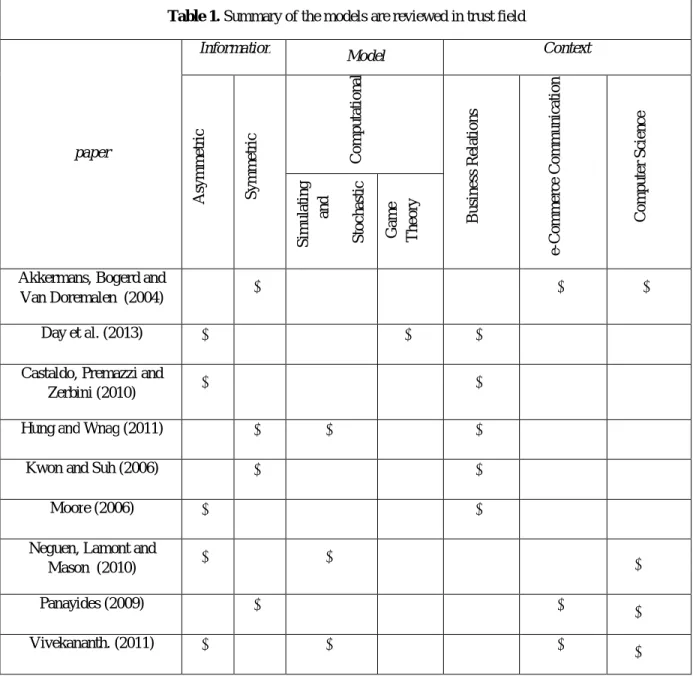
The trust in Computer Science derives from the concept in sociological, psychological and economical environments. The definition of trust is not unique and it may vary depending on the context and the purpose. Nguyen, Zhao and Yang (2010) integrated objective and mental trust in services of an on line network. This model proposed limitations based on trust. As a result, according to the numerical example, customers can choose the best option in service network. Vivekananth. (2011) considered an advanced form of calculating trust for the security of on line networks. He developed a trust model based on appropriate selections under reputation. Therefore, the nodes were selected based on the level of trust. The summaries of trust literature are shown in table 1.
Table 1. Summary of the models are reviewed in trust field Context Model Information paper Com pu te r S ci e n c e e -Co m m e rc e Com m un ic a ti on Bus ine ss Re la ti ons Com pu ta ti on a l S ym m e tr ic A sym m e tr ic G a m e T he o ry S im ul a ti ng a nd S toc h a st ic ، Akkermans, Bogerd and
Van Doremalen (2004) Day et al. (2013)
Castaldo, Premazzi and
Zerbini (2010) Hung and Wnag (2011)
Kwon and Suh (2006)
Moore (2006) Neguen, Lamont and
Mason (2010) Panayides (2009) Vivekananth. (2011)
2.2. Newsvendor problem
The newsvendor problem is one of the classical problems in the literature on inventory management. Key insights stemming from an analysis of this problem have wide ranging implications for managing inventory decisions for organizations in, for example, the hospitality, airline, and fashion goods industries. In the classic model, preparing products is done once at the beginning of a single period and the retailer determines the optimal order quantity and the supplier specifies the optimal wholesale price. (Khouja, 1999).
2.3. Stackelberg game
When we confront a lot of economic, social, political and military issues, we often have to analyze opposite situations. In fact, game theory is a mathematical theory for conflicting or competitive situations. This theory provides rational solutions to optimize decision making (Shakuri and Menhaj, 2008).
Stackelberg game is a kind of game theory which analyzes interactions among leaders and followers which was proposed by Von Stackelberg in 1934. In classic problems, the follower determines his optimal strategy, then the leader determines his optimal strategy based on the best optimal strategy of the follower (Romp, 1997). If the optimal strategies are accepted by the leader and the follower, the game will be over. Otherwise, the game continues until the sides are satisfied (Petruzzi, 1999). Although this game seems to be easy, the payoff matrix can be considerably more difficult to analyze mathematically (Binmore,1998 and Shubik, 2006).
2.4. Newsvendor literature
Most typically, subjects anchor their order quantities to the expected demand in cases where maximal profits could be achieved by ordering much more than the expected demand (if product has a high profit margin, i.e., shortage is relatively more costly than excess) or less than the expected demand (if product has a low profit margin). Qin et al. (2011) call for more studies of the newsvendor problem under both stochastic demand and stochastic supply. In general, uncertain supply either related to procurement (order) or production (production batch order) has been discussed in the inventory management literature. Stochastic yield has been considered in the newsvendor setting for both single and multi-supplier case. For example, Keren and Piliskin (2006) presents how stochastic yield impacts supply chain coordination. Lau, Hasija and Bearden (2014) analyze two newsvendor experiments and find that less than half of subjects suffer from pull-to-center bias. They conclude that there can be significant differences between the subjects within one experiment and urge researchers not to make too strong conclusions from averages across experiments.
In the SCs, which don’t follow the classic law in SCM, members seem to be more leader-follower. It means these SCs face a Stackelberg game. Trust intensifies the effect of leader-follower
relationships because the follower insists on having cooperation under any conditions (advantage or disadvantage).
Li, Li and Cai (2012) offered a SC where the retailer faces a stochastic demand and orders from the supplier, while the supplier manufactures new products and also remanufactures return to meet the order. They used Stackelberg game, where the manufacturing quantity is determined by the supplier after realizing the order quantity from the retailer. They attained that in the Stakelberg game the order and manufacturing quantities are larger than in the inaccessible return information case, and the profits for the supplier and retailer are also higher. Computational results are reported to show the effects of system parameters.
The newsvendor model is probably the most celebrated model in inventory literature and is applied extensively to investigate inventory centralization, cooperation and coordination.
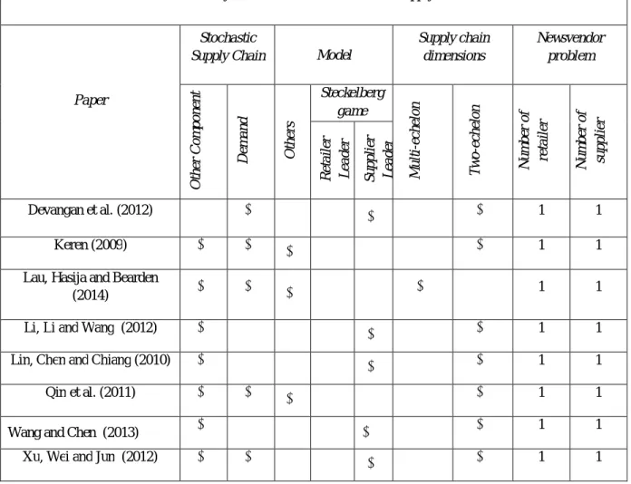
Lin et al. (2010) considered the newsvendor SC problem which was formulated as a Stackelberg game: the manufacturer is the leader who designs a contract or a trade term, and the retailer was the follower who determines the order quantity and selling price. In addition, the perishable retailing problem was formulated as a two-period inventory system. They developed profit of maximization models by taking into account the return policy and quantity discount that are offered by the manufacturer to the retailer. With properly designed contracts, the inefficiency caused by double marginalization can be completely eliminated and, as a result, the SC is coordinated. Devangan et al. (2012) considered a SC coordination problem when demand faced by a retailer is influenced by the amount of inventory displayed on the retail shelf. The goal in this research was to design individually rational contracts that coordinated the SC when the retailer faced inventory-level-dependent demand. They presented a buyback contract where any leftover inventory at the retailer could be returned to the supplier at a pre-specified terms of the buyback contract. They provided managerial insights into the design of the contracts and analyzed the impact of shelf space inventory on the contract parameters. The summeries of newsvendor literature are shown in table 2.
The authors try to to investigate theses aims as follow: First, we try to study a reasonable trust model (Beta model) to calculate amount of trust that is adaptable in SCs. Second, some criteria which to win trust are proposed and for both of the retailer and the supplier a criterion is considered. Finally, a two-echelon SC including a supplier and a retailer with stochastic demand in newsvendor framework is presented. The members play Stackelberg game in which the supplier is the leader and the retailer is the follower. In addition, trust affects the stock level of supplier and the order quantity of retailer and decreases both of them. What’s more, the optimal order quantity of retailer is the demand of supplier.
3. Beta model
The most important component of a probabilistic trust model is the treatment of model to estimate probabilistic future of outputs. Beta model was provided by Jøsang ans Sanderud (2003). According to this model, the trustee’s behavior is a random variable having specific probability distribution. Outputs are successes and failures
3.1. Parameters of Beta model
Validation parameter of trustee having prior mixed beta distribution. Validation parameter of trustee having prior mixed beta distribution. Parameter of post beta distribution.
Table 2 .Summary of the models are reviewed in supply chains field
Newsvendor problem Supply chain
dimensions Model
Stochastic Supply Chain Paper
Num
be
r
of
suppl
ie
r
Num
be
r
of
re
tai
le
r
T
wo
-e
che
lon
M
ul
ti
-e
c
h
e
lon
Steckelberg game
O
the
rs
D
e
m
and
O
the
r
Com
pon
e
n
t
Suppl
ie
r
L
e
ade
r
R
e
tai
le
r
L
e
ade
r
1 1
Devangan et al. (2012)
1 1
Keren (2009)
1 1
Lau, Hasija and Bearden (2014)
1 1
Li, Li and Wang (2012)
1 1
Lin, Chen and Chiang (2010)
1 1
Qin et al. (2011)
1 1
Wang and Chen (2013)
1 1
Parameter of post beta distribution.
ℎ Bernoulli sequence from specific number of interactions including cooperation and none-cooperation for trustee.
(ℎ) Number of cooperation for trustee in specific transactions.
(ℎ) Number of none-cooperation for trustee in specific transactions.
(ℎ) Number of total interacts.
Θ Bayesian parameter estimation. Probability of success in a transition.
Output including cooperation or defect = 1 … . Number of successes (cooperation).
We have a sequence of successes and failures in which the sequence is estimated by Bayesian parameter estimationΘ . The sequence can be suggested by a probabilistic distribution that is the probability of success in a transition. Under the assumption, ℎ = … is a sequence of outputs considered as a Bernoulli trial, and successes follow binomial distribution. (Gelman and Buchwald, 2003).
(1)
(
)
n
te(1
te)
n kP k successes
k
Taking ( )from the beta family, a two-parameter class of distributions can be expressed as follow: (Casella et al. 2003)
(2)
1 1
(
)
(
,
)
(1
)
(
) (
)
pr pr
pr pr
te pr pr te te
pr pr
f
If , is selected as a prior distribution, post distribution of will be a binomial distribution with ( , ) parameters. Thus prior parameters and post parameters are related to each other as follow:
(3) ( )
( ) p o s t s R p r p o s t f R p r
N h
N h
(ℎ), (ℎ) are the cooperation and the defect in ℎ sequence respectively. Trust is the expected value of the post distribution (Jøsang and Sandrud, 2012).
(4)
(
te)
post post postTRUST
E
4. The proposed model
A relationship based on trust between two members of SCs includes the reliability of the two members and the ability of each member to create trust on the opposite side.
4.1. The assumptions
Assumption 1. Utility functions and order quantities are none-negative.
Assumption 2. The model uses exact optimization approach so it is limited to classic techniques. Assumption 3. Trust is an exogenous parameter for the SC.
Assumption 4. Trust as a variable is multiplied in stock level for supplier and order quantitylevel for retailer. We assume that the trust decline the stock of the supplier and the order quantity of the retailer.
Assumption 5. < <
Unit production cost of supplier
Retailer price
Unit wholesale price of supplier
When members of the SC deal, the rated parameters of deal should be specified. If these parameters are not exactly determined, every member will decide based on their opinion. Therefore, there are some criteria which create trust in a SC for both retailer and supplier in a transact. For instance, price, quality, delivery time, payment, unreasonable criticizing, public charity performances and customer services, etc. can be applied as a trust factor.
In this study, payment is a factor which creates trust for the supplier. In other words, the supplier relies on the retailer under specified conditions that is proposed in the contract. Delivery time is a factor the retailer relies on the supplier. Simply put, the retailer trusts the supplier when he delivers services on time.
4.2. Definitions of variables
Stochastic demand with normal distribution with mean , vaiance . The retail price of retailer.
√ Trust function.
Trust of retailer to supplier. Trust of supplier to retailer.
ℎ Unit inventory cost (mitigated by salvage cost) is incurred for units left over at the end of period for retailer.
ℎ Shortage cost per unit of unsatisfied demand is incurred for retailer. The unit wholesale price of supplier.
Initial demand (fixed). Utility function of retailer.
( ) Distribution function of demand.
( ) Cumulative function of demand. The unit Production cost of supplier. Initial stock (fixed).
Order quantity of supplier.
ℎ Unit inventory cost (mitigated by salvage cost) is incurred for units left over at the end of period for supplier.
ℎ Shortage cost per unit of unsatisfied demand for supplier. Utility function of supplier.
4.3. decision variables
Order quantity for retailer.
Inventory quantity for supplier = − + . Stock of supplier.
4.4. The retailer model
Normally, the customer is assumed to be independent of the supplier. It means that the customer does not have any information about the supplier. However, in some special positions, the customer may plan based on the supplier’s inventory. Therefore, we assume the order quantity of retailer decreases by the stock of supplier and the trust.
The retailer model considers the following problem
(6)
2
0 1 ( , )
R
RS RS
m m
D a q N
Tr SS Tr SS
Trust is assumed to decline the order quantity of the retailer. It seems to be correct because a lot of retailers order more than their needs in each ordering in the real cases.
Retailer utility function is:
(7)
[min( , ) ( ) ( )]
R R R R R R R
Max Max E D q h q D h Dq wq
0
( )( ) ( ) ( )
( ) 1 ( )
R R
RS
R RS
m
q a q
T SS
R R R
RS
R
m q a
Tr SS
m
Max p w a q w h F d
Tr SS
p h w F d
Since the retailer seeks maximum profit, the utility function should be concave. Therefore, at first, we calculate derivative of the utility function:
(8)
( ) [( )(1 ) ( [ ])]
[ ( )(1 )[1 ( [ ])]
R
R R R
R RS RS RS
R R
RS RS
m m m
p w w h F q a q
q Tr SS Tr SS Tr SS
m m
p h w F q a
Tr SS Tr SS
Then the second derivative of the utility function is obtained as the follow:
(9)
2 2
2
[( )(1 ) ( [ ])]
2
[( )(1 ) ( [ ])] 0
R
R R R
R RS RS
R R R
RS RS
m m
w h f q a q
q Tr SS Tr SS
m m
p h w f q a q concave
Tr SS Tr SS
Finally, the optimal order quantity is acquired as bellow:
0
[( )(1 ) ( [ ])]
[( )(1 ) ( [ ])] ( ) ( )(1 )
R R
R R R
RS RS
R R R R
RS RS RS RS
q
m m
w h F q a q
Tr SS Tr SS
m m m m
p h w F q a q p w p h w
Tr SS Tr SS Tr SS Tr SS
( [ ])[( )(1 ) ( )(1 )]
( ) ( )(1 )
R R R R
RS RS RS
R
RS RS
m m m
F q a q p h w w h
Tr SS Tr SS Tr SS
m m
p w p h w
Tr SS Tr SS
( ) ( )(1 )
( )
( )(1 ) ( )(1 )
R
RS RS
R R
RS
R R
RS RS
m m
p w p h w
Tr SS Tr SS
m
F q a q
m m
Tr SS p h w w h
Tr SS Tr SS
(10)
1 *
( ) ( )(1 )
( )
( )(1 ) ( )(1 )
(1 )
R
RS R S
R R
RS RS
R
RS
m m
p w p h w
Tr SS Tr SS
F
m m
p h w w h
Tr SS Tr SS
q
m Tr SS
4.5. The supplier model
In fact the order quantity of the retailer is the demand of the supplier. The remarkable thing is that the demand is stochastic, but in the current models, the order quantity is considered deterministic. This assumption seems to be incorrect in the real world. Demand is stochastic; hence, the order quantity also should be practically random.
In the proposed model, order quantity is provided based on a crisp measure of a stochastic variable. The amount has confidence level=1/2 because it is an expected value. In other words, fifty percent is the probability that the order quantity to be higher than the expected value and faces shortage, and also fifty percent is the possibility which I will bet higher than the expected value and faces some extra quantity. Thus, ∗ is not the order quantity for the supplier. In fact, it is the average of the order quantity of the supplier.
The supplier model is suggested as follow:
(11) * 2
( R , )
S
q N q
It is assumed that trust function reduces the stock, so according to this assumption, the inventory of supplier is obtained as follow:
(12)
(
(
))
S SR S
I
b K Tr
ss q
(13)
( )min(( ) , )
(( ) ) (( ) ) ( ( ) )
SR S
S
S SR S S SR S S S SR
E w c b Tr SS q
Max Max
h b Tr SS q h b Tr SS q h q b Tr SS
( )
0 ( )
( ) ( ) 0 0 ( ) ( ) ( ) ( ) ( ( ) ) ( ) (( ) ) ) ( ) SR SR SR SR b Tr
S S S SR S S
b Tr S
b Tr b Tr
S S SR S S S SR S S S
q f q dq b Tr f q dq
w c
h q b Tr SS f q dq h b Tr SS q f q dq
Because the supplier will seeks maximum profit, the utility function should be concave. The derivative of the supplier utility function is:
(14)
( )
( )
0 ( )
( ) ( ) ( ) ( ) ( ) ( ) ( ) SR SR SR S
SR S S b Tr SS
b Tr SS
S SR S S S SR S S
b Tr SS
w c b Tr f q dq
SS
h b Tr f q dq h b Tr f q dq
Second derivative of the supplier utility function is:
(15) 2 2 2 2 2 ( ) (( ) ) ( ) ( ) (( ) ) ( ) (( ) ) S SR SR
S SR SR S SR SR
b Tr f b Tr SS w C
SS
h b Tr f b Tr SS h b Tr f b Tr SS Concave
Optimal inventory of the supplier is:
( )
( )
0 ( )
( ) ( ) ( ) ( ) ( ) ( ) ( ) S R S R S R S
S R S S b T r S S
b T r S S
S S R S S S S R S S
b T r S S
w c b T r f q d q
S S
h b T r f q d q h b T r f q d q
(16) 1 * ( ) ( ) ( ) ( ) ( )S R S
S S R S S R
S R
w c b T r h
F
w c h b T r h b T r
S S
b T r
(17)
* 1 ( ) *
( )
( ) ( )
SR S
S S
S SR S SR
w c b Tr h
I F q
w c h b Tr h b Tr
If optimal amounts are accepted by two sides, the game will be over, and if the optimal amounts are not accepted, the game will be continued.
5. A numerical example for solving the model
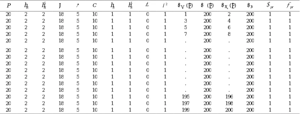
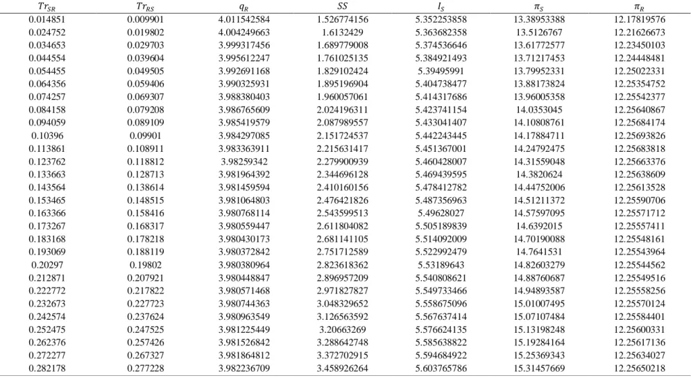
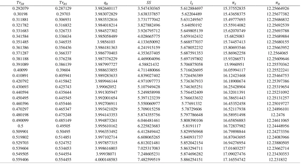
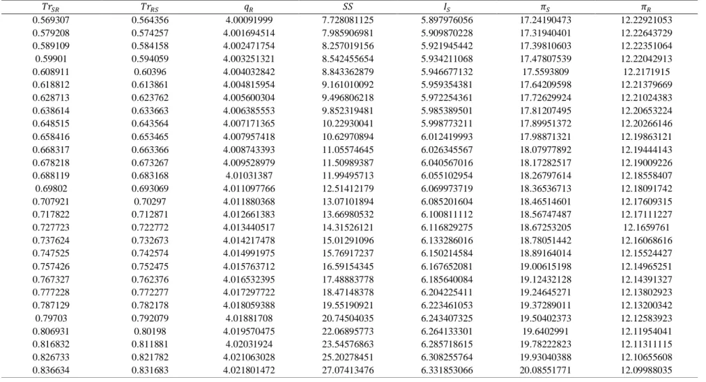
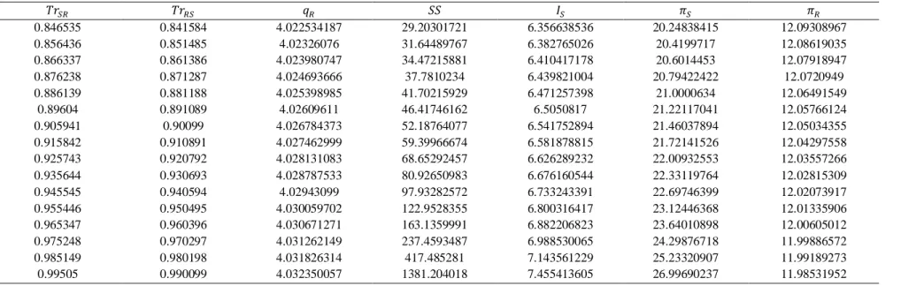
In this section, the model is solved by a numerical example. The default values of parameters for solving the model are presented in table 3.Since trust is considered as a variable parameter, the decision variables and utility functions for both supplier and retailer are calculated by different values of trust. This model is solved by Matlab and is results are presented in table A4 (see appendix A).
5.1. Retailer
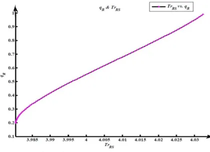
The surge in retailer’s trust enhances order quantity. This rise is non-linear and ascending Figure 1. The utility function has irregular trend. First, it is ascending and then linear in a small interval. Overall, it has a downward trend Figure 2.
Table 3.default value of parameters
pr
pr
(ℎ)(ℎ) (ℎ)
2
Sh
Sh
C Rh
Rh
P
1 1 200 2 200 1 1 0 1 1 10 5 18 2 2 20 1 1 200 4 200 3 1 0 1 1 10 5 18 2 2 20 1 1 200 6 200 5 1 0 1 1 10 5 18 2 2 20 1 1 200 8 200 7 1 0 1 1 10 5 18 2 2 20 1 1 200 . 200 . 1 0 1 1 10 5 18 2 2 20 1 1 200 . 200 . 1 0 1 1 10 5 18 2 2 20 1 1 200 . 200 . 1 0 1 1 10 5 18 2 2 20 1 1 200 . 200 . 1 0 1 1 10 5 18 2 2 20 1 1 200 . 200 . 1 0 1 1 10 5 18 2 2 20 1 1 200 . 200 . 1 0 1 1 10 5 18 2 2 20 1 1 200 . 200 . 1 0 1 1 10 5 18 2 2 20 1 1 200 . 200 . 1 0 1 1 10 5 18 2 2 20 1 1 200 196 200 195 1 0 1 1 10 5 18 2 2 20 1 1 200 198 200 197 1 0 1 1 10 5 18 2 2 20 1 1 200 200 200 199 1 0 1 1 10 5 18 2 2 20Figure 2. Retailer utility function vs. trust
5.2. Supplier
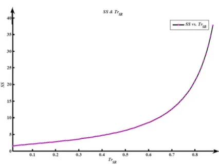
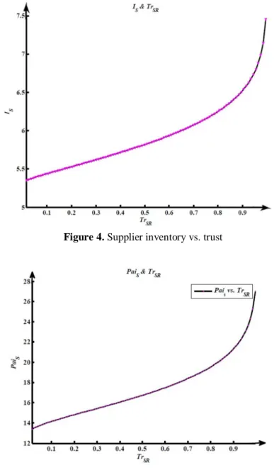
The Stock, inventory and utility functions of the supplier have raised by increasing trust ascend Figure 3, 4 and 5.
Figure 4. Supplier inventory vs. trust
Figure 5. Supplier utility function vs. trust
6. CONCULSION
In this research, we proposed a mathematical trust model in the SC. We found several components such as price, quality, delivery time, payment, after sales services, unreasonable criticizes and public charity performance to create trust for both retailer and supplier. This research assumes that the supplier gains trust when the retailer pays financial bills according to their contract. The retailer also trusts when the supplier sends its orders without delay. We assumed trust as a variable parameter which was computed by Beta model. The Beta model was the most compatible with the computational trust model for calculating trust. Trust reduces stock and order quantity in demand function. Finally, a numerical example was solved to investigate the efficiency of the model. In conclusion, we found that more trust made the stock grew considerably and according to the model optimal order quantity depends on stock. In fact, non-linear and ascending approach of stock causes
the optimal order quantity to increase as well. The retailer utility function had generally a downward trend. Simply put, the retailer did not achieve profit in this process. In the supplier model, where there is more trust, the utility function, inventory, and stock also enhance because these variables directly depend on each other. In other words, the supplier gains significantly more profit. To sum up, another flow was proposed to the SC that may have led to more profit and as a facilitator can cut extra costs and accelerate operations in SCs.
References
Akkermans, H., Bogerd, P., & Van Doremalen, J. (2004). Travail, transparency and trust: A
case study of computer-supported collaborative supply chain planning in high-tech
electronics. European Journal of Operational Research, 153(2), 445-456.
Binmore, K. G. (1998). Game theory and the social contract: Playing fair (Vol. 2). The MIT
Press
.Casella, R. (2003). Zero tolerance policy in schools: Rationale, consequences, and
alternatives. The Teachers College Record, 105(5), 872-892
Castaldo, S., Premazzi, K., & Zerbini, F. (2010). The meaning (s) of trust. A content analysis
on the diverse conceptualizations of trust in scholarly research on business relationships.
Journal of Business Ethics, 96(4), 657-668.
Day, M., Fawcett, S. E., Fawcett, A. M., & Magnan, G. M. (2013). Trust and relational
embeddedness: Exploring a paradox of trust pattern development in key supplier
relationships Industrial Marketing Management
.Devangan, L., Amit, R. K., Mehta, P., Swami, S., & Shanker, K. (2012). Individually rational
buyback contracts with inventory level dependent demand. International Journal of
Production Economics.
Di, X., Wei, D., & Yun-hong, H. (2012). Buy Back Contract Based on Quality Effort in
Supply chain. In Frontiers in Computer Education (pp. 313-323). Springer Berlin Heidelberg
Esfandiari, B., & Chandrasekharan, S. (2001, May). On how agents make friends:
Mechanisms for trust acquisition. In Proceedings of the Fourth Workshop on Deception,
Fraud and Trust in Agent Societies, Montreal, Canada (pp. 27-34).
Gambetta, D. (1990). Trust: Making and breaking cooperative relations
Gelman, D., & Buchwald, S. L. (2003). Efficient palladium
‐
catalyzed coupling of aryl
chlorides and tosylates with terminal alkynes: Use of a copper cocatalyst inhibits the reaction
Angewandte Chemie International Edition, 42(48), 5993-5996
.Hassan, J., Sirisena, H., & Landfeldt, B. (2008). Trust-based fast authentication for multi-
wireless networks. Mobile Computing, IEEE Transactions on, 7(2), 247-261.
Hung, H. C., & Wang, T. W. (2011). Determinants and mapping of collective perceptions of
technological risk: the case of the second nuclear power plant in Taiwan. Risk analysis,
31(4), 668-683.
Huynh, T. D., Jennings, N. R., & Shadbolt, N. R. (2006, May). Certified reputation: how an
Agent can trust a stranger. In Proceedings of the fifth international joint conference on
Autonomous agents and multiagent systems (pp. 1217-1224). ACM
.Jøsang, A., & Sanderud, G. (2003, January). Security in mobile communications: challenges
and opportunities. In Proceedings of the Australasian information security workshop
conference on ACSW frontiers 2003-Volume 21 (pp. 43-48). Australian Computer
Society,Inc
.Kamvar, S. D., Schlosser, M. T., & Garcia-Molina, H. (2003, May). The eigentrust algorithm
for reputation management in p2p networks. In Proceedings of the 12th international
conference on World Wide Web (pp. 640-651). ACM
Keren, B. and Pliskin, J. S. (2006). A benchmark solution for the risk-averse vendorproblem.
European Journal of Operational Research, 174(3):1643–1650.
Khouja, M. (1999). The single-period (news-vendor) problem: literature review and
suggestions for future research. Omega, 27(5), 537-553
.Kwon, I. W. G., & Suh, T. (2004). Factors affecting the level of trust and commitment in
supply chain relationships. Journal of Supply Chain Management, 40(1), 4-14.
Lau, N., Hasija, S., & Bearden, J. N. (2014). Newsvendor pull-to-center reconsidered.
Decision Support Systems, 58, 68-73.
Lewis, J. D., & Weigert, A. (1985). Trust as a social reality. Social forces, 63(4), 967-985.
Li, X., Li, Y., & Cai, X. (2012). Quantity decisions in a supply chain with early returns
remanufacturing. International Journal of Production Research, 50(8), 2161-2173
.Lin, Y. H., Chen, J. M., & Chiang, T. C. (2010). Channel coordination for a newsvendor
problem with return and quantity discount. Journal of Information and Optimization Sciences
31(4), 857-873.
Mcknight, D. H. and Chervany, N. L. “The meanings of trust: University of Minnesota,
Technical reports
”.http://misrc.umn.edu/wpaper/WorkingPapers/9604.pdf, 1996.
Marsh, S. (1994). Trust in distributed artificial intelligence. In Artificial Social Systems (pp.
94-112). Springer Berlin Heidelberg.
Mejia, M., ChaparroVargas, R. (2013). Distributed Trust and Reputation Mechanisms for
Vehicular Ad-Hoc Networks.
Nguyen, D. Q., Lamont, L., & Mason, P. C. (2009). On trust evaluation in mobile ad-hoc
networks. In Security and Privacy in Mobile Information and Communication Systems (pp.
1-13). Springer Berlin Heidelberg
Nguyen, H. T., Zhao, W., & Yang, J. (2010, July). A trust and reputation model based on
bayesian network for Web services. In
Web Services (ICWS), 2010 IEEE International
Conference on
(pp. 251-258). IEEE.
Panayides, P. M., & Venus Lun, Y. H. (2009). The impact of trust on innovativeness and
supply chain performance. International Journal of Production Economics, 122(1), 35-46.
Petruzzi, N. C., & Dada, M. (1999). Pricing and the newsvendor problem: A review with
extensions. Operations Research, 47(2), 183-194
.Qin, Y., Wang, R., Vakharia, A. J., Chen, Y., & Seref, M. M. (2011). The newsvendor
problem: Review and directions for future research. European Journal of Operational
Research, 213(2), 361-374.
Romp, G. (1997). Game theory: introduction and applications. OUP Catalogue.
Shakouri, H., Menhaj, M.B. (2008). “A single fuzzy rule to smooth the sharpness of mixed
Data: Time and frequency domains analysis”, Fuzzy Sets & Systems (FSS), No. 159, pp.
2446 -2465
.Shubik, M. (2006). Game theory in the social sciences: Concepts and solutions.
Staples, D. S., & Webster, J. (2008). Exploring the effects of trust, task interdependence and
virtualness on knowledge sharing in teams. Information Systems Journal, 18(6), 617-640
.Vivekananth, P. (2011, May). Enhanced reliable trust model for grid computing based on
reputation. In Proceedings of the 2011 international conference on Computers and computing
(pp. 39-45). World Scientific and Engineering Academy and Society (WSEAS).
Wang, C., & Chen, X. (2013). Fresh Produce Supply Chain Management Decisions with
Circulation Loss and Options Contracts. In
LISS 2012
(pp. 643-647). Springer Berlin
Heidelberg.
Wang, Y., & Singh, M. P. (2007, January). Formal Trust Model for Multiagent Systems. In
IJCAI (Vol. 7, pp. 1551-1556).
Williamson, O. E. (1993). Calculativeness, trust, and economic organization. Journal of law
and economics, 453-486.
Xu, J., Wei, J., & Jun, T. (2012). Comparing improvement strategies for inventory
inaccuracy in a two-echelon supply chain. European Journal of Operational Research, 221(1),
213.
Appendix A
Table A4. Results of solving example
12.17819576 13.38953388 5.352253858 1.526774156 4.011542584 0.009901 0.014851 12.21626673 13.5126767 5.363682358 1.6132429 4.004249663 0.019802 0.024752 12.23450103 13.61772577 5.374536646 1.689779008 3.999317456 0.029703 0.034653 12.24448481 13.71217453 5.384921493 1.761025135 3.995612247 0.039604 0.044554 12.25022331 13.79952331 5.39495991 1.829102424 3.992691168 0.049505 0.054455 12.25354752 13.88173824 5.404738477 1.895196904 3.990325931 0.059406 0.064356 12.25542377 13.96005358 5.414317686 1.960057061 3.988380403 0.069307 0.074257 12.25640867 14.0353045 5.423741154 2.024196311 3.986765609 0.079208 0.084158 12.25684174 14.10808761 5.433041407 2.087989557 3.985419579 0.089109 0.094059 12.25693826 14.17884711 5.442243445 2.151724537 3.984297085 0.09901 0.10396 12.25683818 14.24792475 5.451367001 2.215631417 3.983363911 0.108911 0.113861 12.25663376 14.31559048 5.460428007 2.279900939 3.98259342 0.118812 0.123762 12.25638609 14.3820624 5.469439595 2.344696128 3.981964392 0.128713 0.133663 12.25613528 14.44752006 5.478412782 2.410160156 3.981459594 0.138614 0.143564 12.25590706 14.51211372 5.487356963 2.476421826 3.981064803 0.148515 0.153465 12.25571712 14.57597095 5.49628027 2.543599513 3.980768114 0.158416 0.163366 12.25557411 14.6392015 5.505189839 2.611804082 3.980559447 0.168317 0.173267 12.25548161 14.70190088 5.514092009 2.681141105 3.980430173 0.178218 0.183168 12.25543964 14.7641531 5.522992479 2.751712589 3.980372842 0.188119 0.193069 12.25544562 14.82603279 5.53189643 2.823618362 3.980380964 0.19802 0.20297 12.25549516 14.88760687 5.540808621 2.896957209 3.980448847 0.207921 0.212871 12.25558256 14.94893587 5.549733466 2.971827827 3.980571468 0.217822 0.222772 12.25570124 15.01007495 5.558675096 3.048329652 3.980744363 0.227723 0.232673 12.25584401 15.07107484 5.567637414 3.126563592 3.980963549 0.237624 0.242574 12.25600331 15.13198248 5.576624135 3.20663269 3.981225449 0.247525 0.252475 12.25617136 15.19284164 5.585638822 3.288642748 3.981526842 0.257426 0.262376 12.25634027 15.25369343 5.594684922 3.372702915 3.981864812 0.267327 0.272277 12.25650218 15.31457669 5.603765786 3.458926264 3.982236709 0.277228 0.282178
Appendix A
Table A4. Results of solving example
12.25664926 15.37552835 5.612884697 3.547430365 3.982640117 0.287129 0.292079 12.25677382 15.43658375 5.62204489 3.638337857 3.983072829 0.29703 0.30198 12.25686832 15.49777693 5.631249567 3.731777042 3.983532816 0.306931 0.311881 12.25692539 15.55914082 5.64050192 3.827882496 3.984018214 0.316832 0.321782 12.25693788 15.62070749 5.649805139 3.926795712 3.984527302 0.326733 0.331683 12.25689884 15.6825083 5.659162432 4.028665775 3.985058489 0.336634 0.341584 12.25680155 15.74457413 5.668577037 4.133650092 3.9856103 0.346535 0.351485 12.25663952 15.80693546 5.678052232 4.241915159 3.986181363 0.356436 0.361386 12.2564065 15.86962258 5.687591353 4.353637405 3.986770403 0.366337 0.371287 12.25609646 15.93266571 5.697197802 4.469004096 3.987376229 0.376238 0.381188 12.25570362 15.9960951 5.706875058 4.58821432 3.987997727 0.386139 0.391089 12.25522241 16.05994117 5.716626695 4.711480066 3.988633855 0.39604 0.40099 12.25464753 16.12423468 5.726456389 4.839027402 3.989283633 0.405941 0.410891 12.25397386 16.18900674 5.736367933 4.971097773 3.989946144 0.415842 0.420792 12.25319654 16.25428904 5.746365251 5.107949428 3.99062052 0.425743 0.430693 12.25231092 16.32011391 5.756452409 5.249858998 3.991305947 0.435644 0.440594 12.25131257 16.38651443 5.766633632 5.397123239 3.992001654 0.445545 0.450495 12.25019727 16.45352458 5.77691332 5.550060977 3.992706911 0.455446 0.460396 12.24896101 16.52117938 5.78729606 5.709015258 3.993421029 0.465347 0.470297 12.2476 16.58951498 5.797786648 5.874355756 3.994143353 0.475248 0.480198 12.24611065 16.65856883 5.808390106 6.046481461 3.994873261 0.485149 0.490099 12.24448956 16.72837982 5.8191117 6.225823683 3.995610162 0.49505 0.5 12.24273356 16.79898844 5.829956968 6.412849442 3.996353492 0.50495 0.509901 12.24083966 16.87043695 5.840931737 6.608065265 3.997102714 0.514851 0.519802 12.23880505 16.94276954 5.852042154 6.812021481 3.997857315 0.524752 0.529703 12.23662714 17.01603257 5.863294711 7.025317083 3.998616803 0.534653 0.539604 12.23430353 17.09027476 5.874696282 7.248605231 3.99938071 0.544554 0.549505 12.231832 17.16554742 5.886254151 7.482599519 4.000148583 0.554455 0.559406
Appendix A
Table A4. Results of solving example
12.22921053 17.24190473 5.897976056 7.728081125 4.00091999 0.564356 0.569307 12.22643729 17.31940401 5.909870228 7.985906981 4.001694514 0.574257 0.579208 12.22351064 17.39810603 5.921945442 8.257019156 4.002471754 0.584158 0.589109 12.22042913 17.47807539 5.934211068 8.542455654 4.003251321 0.594059 0.59901 12.2171915 17.5593809 5.946677132 8.843362879 4.004032842 0.60396 0.608911 12.21379669 17.64209598 5.959354381 9.161010092 4.004815954 0.613861 0.618812 12.21024383 17.72629924 5.972254361 9.496806218 4.005600304 0.623762 0.628713 12.20653224 17.81207495 5.985389501 9.852319481 4.006385553 0.633663 0.638614 12.20266146 17.89951372 5.998773211 10.22930041 4.007171365 0.643564 0.648515 12.19863121 17.98871321 6.012419993 10.62970894 4.007957418 0.653465 0.658416 12.19444143 18.07977892 6.026345567 11.05574645 4.008743393 0.663366 0.668317 12.19009226 18.17282517 6.040567016 11.50989387 4.009528979 0.673267 0.678218 12.18558407 18.26797614 6.055102954 11.99495713 4.01031387 0.683168 0.688119 12.18091742 18.36536713 6.069973719 12.51412179 4.011097766 0.693069 0.69802 12.17609315 18.46514601 6.085201604 13.07101894 4.011880368 0.70297 0.707921 12.17111227 18.56747487 6.100811112 13.66980532 4.012661383 0.712871 0.717822 12.1659761 18.67253205 6.116829275 14.31526121 4.013440517 0.722772 0.727723 12.16068616 18.78051442 6.133286016 15.01291096 4.014217478 0.732673 0.737624 12.15524427 18.89164014 6.150214584 15.76917237 4.014991975 0.742574 0.747525 12.14965251 19.00615198 6.167652081 16.59154345 4.015763712 0.752475 0.757426 12.14391327 19.12432128 6.185640084 17.48883778 4.016532395 0.762376 0.767327 12.13802923 19.24645271 6.204225411 18.47148378 4.017297722 0.772277 0.777228 12.13200342 19.37289011 6.223461053 19.55190921 4.018059388 0.782178 0.787129 12.12583923 19.50402373 6.243407325 20.74504035 4.01881708 0.792079 0.79703 12.11954041 19.6402991 6.264133301 22.06895773 4.019570475 0.80198 0.806931 12.11311115 19.78222823 6.285718615 23.54576863 4.02031924 0.811881 0.816832 12.10655608 19.93040388 6.308255764 25.20278451 4.021063028 0.821782 0.826733 12.09988035 20.08551771 6.331853066 27.07413476 4.021801472 0.831683 0.836634
Appendix A
Table A4. Results of solving example
12.09308967 20.24838415
6.356638536 29.20301721
4.022534187 0.841584
0.846535
12.08619035 20.4199717
6.382765026 31.64489767
4.02326076 0.851485
0.856436
12.07918947 20.6014453
6.410417178 34.47215881
4.023980747 0.861386
0.866337
12.0720949 20.79422422
6.439821004 37.7810234
4.024693666 0.871287
0.876238
12.06491549 21.0000634
6.471257398 41.70215929
4.025398985 0.881188
0.886139
12.05766124 21.22117041
6.5050817 46.41746162
4.02609611 0.891089
0.89604
12.05034355 21.46037894
6.541752894 52.18764077
4.026784373 0.90099
0.905941
12.04297558 21.72141526
6.581878815 59.39966674
4.027462999 0.910891
0.915842
12.03557266 22.00932553
6.626289232 68.65292457
4.028131083 0.920792
0.925743
12.02815309 22.33119764
6.676160544 80.92650983
4.028787533 0.930693
0.935644
12.02073917 22.69746399
6.733243391 97.93282572
4.02943099 0.940594
0.945545
12.01335906 23.12446368
6.800316417 122.9528355
4.030059702 0.950495
0.955446
12.00605012 23.64010898
6.882206823 163.1359991
4.030671271 0.960396
0.965347
11.99886572 24.29876718
6.988530065 237.4593487
4.031262149 0.970297
0.975248
11.99189273 25.23320907
7.143561229 417.485281
4.031826314 0.980198
0.985149
11.98531952 26.99690237
7.455413605 1381.204018
4.032350057 0.990099