Vol. 2, No. 3, pp 197-213 Fall 2008
COVERT Based Algorithms for Solving the Generalized Tardiness Flow
Shop Problems
Farhad Ghassemi-Tari1*, Laya Olfat2
1
Department of Industrial Engineering, Sharif University of Technology, Iran [email protected]
2
School of Management, Tabatabaei University, Iran [email protected]
ABSTRACT
Four heuristic algorithms are developed for solving the generalized version of tardiness flow shop problems. We consider the generalized tardiness flow shop model with minimization of the total tardiness as its performance measure. We modify the concept of cost over time (COVERT) for the generalized version of the flow shop tardiness model and employ this concept for developing four algorithms. The efficiency of the developed algorithms is then tested through extensive computational experiments and the results will be presented.
Keywords: Sequencing and scheduling, Flow shop, Generalized flow shop, Intermediate due date, Tardiness, COVERT index.
1. INTRODUCTION
This paper considers the generalized tardiness flow shop scheduling model with the total tardiness as its measure of performance (Ghassemi-Tari and Olfat, 2007). In traditional flow shop models the work in a job is broken down into separate tasks called operations, while each operation of a job is performed on different machine in a unidirectional precedence structure. By unidirectional structure we mean that for each operation after the first there is exactly one direct predecessor and for each operation before the last there is exactly one direct successor. The shop contains m different machines and each job consists of m operations each of which requires a different machine. The machines in a flow shop can thus be numbered 1, 2… m; and the operations of job j numbered (1, j), (2, j)… (m, j), so that they correspond to the machine required. For the traditional models with the total tardiness minimization objective, there is a given due date for completion of each job (last operation of each job), and the tardiness of a job is defined as the amount of time by which the completion of the last operation of a job exceeds its associated due date. In the generalized version for every operation of a job there is an associated due date, and the tardiness of each operation of a job is defined as the amount of time by which the completion of each operation of a job exceeds its associated due date.
In the flow shop problem, there are n! job sequences, possible for each machine, and as many as (n!)m schedules. Among these schedules if we consider those by which the same job sequence
*
occurs on each machine we will have the case of the permutation scheduling. In case of the permutation scheduling our effort for finding the best schedule is limited to the search for only n! schedules. In this paper, the developed algorithms consider the case of the permutation scheduling of tardiness flow shop problems.
There are a number of research attempts considering traditional tardiness scheduling problems. The early research efforts are traced back to late 1970’s as shown in the literature survey of Baker and Scudder (1990). Many other tardiness scheduling problems have considered tardiness criteria under common due date circumstances. Common due date scheduling problems, were fist introduced by Kanet (1981a, 1981b). Sundararaghavan and Ahmed (1984) have shown that the optimal schedule generated by Kanet's algorithm can break the zero-ready-time assumption rules if its given due date is restrictively urgent. Hall et al. (1991) have further characterized the optimal schedule properties for the problem of Kanet and have proved that his problem is NP-complete. Some other tardiness scheduling problems have considered batch processing of jobs. Among those, Ahmadi et al. (1992) have investigated a class of flow shop scheduling problems with at least one batch per machine. However, they have done the complexity analysis for two problem instances with make span and mean flow time measures while not considering the tardiness criterion. Later, Mosheiov (2003) extended the problem to a situation in which two elements of “job identical processing time” and “job-dependent weights” were combined and an m-machine flow shop scheduling problem with a given common due date was defined. He considered the (just in time) objective of minimizing the maximum earliness/tardiness cost. He then introduced a polynomial time solution approach for the proposed problem.
Some exact solution algorithms have also been reported for the traditional flow shop scheduling problems (Yeh and Allahverdi, 2004). Karimi (1992) proposed an integer nonlinear programming formulation of multi-stage serial production systems under constant demand and infinite horizon, in which production stages operate with periodic shut-downs and startups. He then showed that the branch and bound algorithm to be the best approach for solving the proposed problem. Faaland and Schmitt (1987) developed an approximate approach for scheduling tasks to minimize lateness penalties in fabrication and assembly processes. They have evaluated their proposed approach through a simulation experiment, in which various fabrication/assembly processes were involved and as the result they indicated that cost improvements occur as the complexity of the scheduling procedure increases.
Currently available heuristic approaches for sequencing jobs in a shop may be classified as either constructive or improvement. A constructive heuristic approach builds a sequence of jobs so that once a schedule is constructed it cannot be reversed. On the other hand, an improvement heuristic approach starts with any sequence of jobs and then attempts to improve the solution by modifying the sequence iteratively. The latter approach has shown to be superior in terms of performance. Several constructive heuristic approaches for the sequencing problem have been proposed by Armentano and Ronconi (1999), and Etiler, Toklu, and Atak (2004).
In this paper we develop four algorithms which are based on the COVERT concept. This concept has been proposed in several studies for single machine and job shop scheduling problems. Among these studies is the earlier work of Carroll (1965) who presented a dynamic rule called COVERT for a single machine and job shop sequencing problems for minimizing the total weighted tardiness of jobs. Under this rule the degree of criticality of jobs were determined by COVERT factor and used for determining jobs sequence. Rachamaduagu and Morton (1982) introduced a rule called apparent tardiness cost (ATC) for single machine sequencing with the total weighted tardiness criteria. Later, Rachamadugu (1984) conducted an experiment for comparing the ATC rule with
COVERT. In his experiment both rules are applied to the single machine, parallel machine and job shop sequencing problems. The experiments demonstrate some circumstances in which ATC provides a better schedule than COVERT.
Vepsalainen and Morton (1987) reached the same conclusion when they compared several sequencing rules consisting of ATC and COVERT rules in solving job shop sequencing problems. They considered job shop problems with tight due dates, lose due dates, and different workloads and concluded that ATC performed better in all of these cases and COVERT had the second best performance among all other rules considered in their experiment. However the power of COVERT in finding a schedule for flow shop problems was not considered in both of studies. Baker (1984, 1987) conducted research studies to evaluate different sequencing rules in job shop scheduling problems. He classified several rules in three groups, namely, slack based, operation-oriented rules and job-oriented rules. He then evaluated different rules of each group and concluded a low performance for the slack based rules, and best performance for the job-oriented rules. The preliminary experiments conducted by Ghassemi-Tari and Olfat (2004) have suggested that COVERT is potentially a promising concept for developing effective heuristic algorithms for solving tardiness scheduling problems.
Sapar and Henry (1996) evaluated six scheduling rules in two machine flow shop problems with the average tardiness criterion. Among these rules, the modified due date rule has been reported to be superior under all variants of the experimental conditions. There are some other classes of heuristic approaches such as CDS algorithms, Tabu search (Bilge, Kirac, Kurtulan, and Pekgun 2004, and Glover 1994), neighboring search (Kim, 1993), and artificial intelligence search method (Lee, 2001).
Review of the existing literature reveals that no unified heuristic algorithm is proposed to perform effectively in solving even the traditional version of tardiness flow shop scheduling problems (Suliman, 2000, and Hall, 2001).
In this paper four heuristic algorithms are developed for solving the generalized version of tardiness flow shop problems. We are considering a generalized tardiness flow shop problem characterized by the following conditions:
•A set of n independent, multiple-operation jobs is available for processing at time zero.
•Each job requires m operations and operation j is performed on machine j and there is a due date associated with the completion of each operation.
•Setup times for the operations are sequence independent and included in processing times.
•The processing times of each operation are known in advance.
•All machines are continuously available.
•Once an operation begins, it proceeds without interruption.
Based on these assumptions four algorithmic procedures are developed and their efficiencies are tested via a set of randomly generated test problems.
2. NOMENCLATURE
The following notations are used throughout this manuscript: pij: Processing time for operation j of job i.
dij; Due date for operation j of job i.
rij: The total processing time of job i on machine 1,2,…,j-1.
tij: The completion time of the j th
operation of the job which is sequenced directly before job i on machine j.
Cij: Completion time of job i on machine j.
xik: Starting time of the k th
operation of job i.
yji: A zero-one variable, which takes 1 if job j precedes job i and takes zero otherwise.
Tik: Tardiness of the kth operation of job i. vi: The expected tardiness of job i.
Sij: The slack time of job i on machine j.
TT: Total tardiness of a schedule. TT(Sj): Total tardiness of schedule Sj.
TTj: Total tardiness of a schedule of all jobs on machine j.
Tk(S): Tardiness of job k in schedule S
Aj: An ordered set of partially scheduled jobs on machine j.
B: A set of unscheduled jobs (complement of Aj).
Sj: A permutation schedule, in which jobs are sequenced according to the order of jobs determined on machine j.
3. MATHEMATICAL FORMULATION OF THE PROBLEM
To present a mathematical programming formulation for the proposed problem, we consider a set of n jobs, each having m operations to be processed on m different machines with a unidirectional precedence structure. In this case we can number machines according to the operation number of each job. Then we will have a one to one correspondence in operation numbers and machine numbers. Therefore as in the case of "pure' flow shop model, the jth operation of each job is performed on the jth machine for all the values of j=1, 2…m. In practical situations however, some jobs may require fewer than m operations, but with the same processing sequence. In such cases for converting the problem to the pure flow shop model, we add some dummy operations for such a job in order to have exactly m operations for each job, while we assign zero value for the processing time of dummy operations.
In the generalized tardiness flow shop model, the shop contains m different machines, and n jobs each consisting of m operations, for each of which there is a due date, called intermediate due date. The problem is considered under the following conditions:
C2. Setup times for the operations are sequence independent and are included in processing times.
C3. Job processing times are known and are deterministic. C4. All machines are continuously available.
C5. No preemption is allowed for individual operations.
Under these conditions we have the basic flow shop model (Baker 1974). The objective is to find a schedule which minimizes the total tardiness. In the generalized tardiness flow shop model, the total tardiness of a schedule is defined by the summation of the individual tardiness of each job when the tardiness of each job is defined by the summation of the tardiness of the individual operation of that job. Let Tik denote the tardiness of the k
th
operation (machine) of job i. The value of Tik is determined as follow:
{
0
,
(
)
}
1
,
2
,
,
1
,
2
,
.
max
x
p
d
i
n
k
m
T
ik=
ik+
ik−
ik∀
=
K
=
K
The mathematical programming model for finding the optimal solution of the problem is presented as follows: m k n i T n j i x n j i or y m k n j i x p x y M m k n j i x p x y M m k n j i x p x My m k n j i x p x My n j i x p x y M n j i x p x My m k n i T d p x T TT ik ij ji ik k i k i ji ik jk jk ji jk k j k j ji jk ik ik ji i j j ji j i i ji ik ik ik ik n j m k ik ≤ ≤ ≤ ≤ ≥ ≤ ≤ ≥ ≤ ≤ = ≤ ≤ ≤ ≤ ≤ + + − − ≤ ≤ ≤ ≤ ≤ + + − − ≤ ≤ ≤ ≤ ≤ + + − ≤ ≤ ≤ ≤ ≤ + + − ≤ ≤ ≤ + + − − ≤ ≤ ≤ + + − ≤ ≤ ≤ ≤ ≤ − + = − − − − = =
∑∑
1 , 1 0 , 1 0 , 1 1 0 2 , , 1 ) 1 ( 2 , , 1 ) 1 ( 2 , , 1 2 , , 1 , 1 ) 1 ( , 1 1 , 1 max min 1 , 1 ., 1 , 1 , 1 1 1 1 1 1 1 1Where M is a very large number.
This mathematical programming model is a combinatorial optimization model. In combinatorial optimization the computational time for obtaining the optimal solution increases exponentially as the number of the decision variables is increased. Since the real-world flow shop problems are formulated as a large scale combinatorial optimization model, the only applicable approach for obtaining a solution is a heuristic approach (Lauff, and Werner, 2004). In this research, the development of such heuristic approaches is considered.
4. PROPOSED ALGORITHMS
Thorough analysis of the generalized tardiness flow shop problem indicates that, the most appropriate indices for sequencing jobs is the use of an index consisting of job processing times and their associated due dates. Therefore, we modify the COVERT index for implementing into our proposed algorithms.
COVERT has been reported as an efficient index for determining the degree of criticality of jobs in increasing the total tardiness of a sequence. Hence it can be used as a measure for finding job sequences where the total tardiness of jobs is used as the measure of performance of a schedule. The effectiveness of this index has been evaluated in a variety of scheduling problems, such as single machine, multiple-machine, flow shop, and job shop scheduling problems. Although this index has been used as a basis for determining a sequence for jobs but no one has used this index for development of an algorithmic procedure for determining the best schedule of the jobs. Further- more the effectiveness of this index has not yet been evaluated for the generalized tardiness flow shop problems.
The original COVERT priority index represents the expected tardiness cost per unit of imminent processing time, or cost over time (Baker 1984, 1987). Job i sequencing for operation j with zero or negative slack is projected to be tardy by completion with an expected tardiness of vi and priority index vi/pij. If, on the other hand, the slack exceeds some generous “worst case” estimate of the waiting time, the expected tardiness cost is set to zero. The worst case waiting time serves as a reference for a piecewise-linear “look ahead”, for a mapping of the expected tardiness cost over the slack Sij:
∑
∑
= =
+ + − ×
=
i i
m
j q
iq m
j q
ij iq
ij i ij
W k
S W k p v t COVERT
] ) ( [
) (
Where Wiq is the expected waiting time for remaining operation q, and k is a multiplier adjusting the expected waiting time to the worst case, say the 99% limiting cumulative probability distribution. The value of k is usually determined through experimental analysis. In most of the research efforts reported in the literature the value of k is set equal to 2.
We employed the structure of the COVERT index and employed the concurrent effect of the job processing time and its due date. We developed several COVERT indices through different relations of job processing times and job due dates, and conducted some preliminary analysis to find the most appropriate mathematical relation for the case of generalized tardiness flow shop problem. We finally chose four mathematical relations which were then incorporated into our proposed algorithms. The modified versions of the COVERT indices are denoted by CVTI, CVTII, CVIII, and CVTIV which are defined as follows:
ij ij ij ij ij ij ij
kbp t d kbp p
t CVTI
+ + − − ×
= 1 [ ( ) ]
) (
ij ij ij ij ij ij ij ij
kbp t d kbp d
p t CVTII
+ + − − ×
= 1 [ ( ) ]
) (
ij ij ij ij
ij ij ij ij
kbp r t d
kbp p
t CVTIII
+ + −
− ×
= 1 [ ( max{ , }) ]
) (
ij ij ij ij
ij ij
ij ij ij
kbp r t d
kbp d
p t CVTIV
+ + −
− ×
= 1 [ ( max{ , }) ]
) (
Through our literature survey we found that the best value for b and k is suggested to be 2 (Baker 1984, 1987). We therefore choose b=2 and k=2, and based on the modifications of the COVERT index we develop four algorithmic procedures for solving the generalized flow shop tardiness problems. We name these algorithms as CO1, … , CO4 in which the COVERT indices of CVTI through CVTIV are employed respectively.
In development of the proposed algorithms, we consider the case of finding permutation schedules. All four algorithms follow a common procedure for finding a permutation schedule. In each algorithm we employ its associate COVERT index and we determine an order of the jobs on machine 1. We then consider machines 2 through m and by using the same COVERT index we determine an order for each individual machine. Through this procedure we identify m different orders of the jobs. We now employ each individual order to determine a permutation schedule of n jobs on m machine. Through this procedure we obtain m different permutation schedules. For each permutation schedule we determine the value of the total tardiness and among these m schedules, the one with smallest total tardiness is selected as the final schedule.
Besides using the different COVERT indices in each algorithm, there is a distinct difference between the first two algorithms, namely CO1 and CO2, and the other tow algorithms, namely CO3 and CO4. In CO1 and CO2, for determining an order for the jobs, we assume that the kthoperation of a job can be started on machine k by the completion of the kth operation of the preceding job on the same machine. In CO3 and CO4, however, we consider a more realistic assumption. That is, the process of the kth operation of a job can not be started on machine k before the completion of k-1operation on machine k-1 and before the completion of the kth operation of its preceding job. Therefore, the starting time for the operation k of a job on machine k is the maximum of the total processing times of its predecessor operations on machine 1 through k-1 and the completion of operation k of its preceding jobs on machine k.
Based on the above concepts, the algorithmic steps of the proposed algorithms can be presented as follows:
Algorithm CO1
Step 1. Let j=1.
Step 2. Let tij=0, TTj=0, Cij=0, Aj=φ, and B={1,2,...,n}. Step 3. Calculate CO1ias follow:
)} ( { max
1 ij ij
B i
i CVTI t
CO ∈
= .
Step 4. Let i be the associated job of CO1i, remove i form B and place it in the last position of Aj.
Step 5. LetCij=tij+pij,andTTj =TTj +max{0,Cij−dij). If B is empty, go to 6, otherwise let
,
ij ij C
t = and go to step 3.
Step 6. Define the permutation schedule Sj, by sequencing jobs according to the jobs’ order of Aj.
Step 7. Let TT(Sj) be defined as the total tardiness of schedule Sj, calculate the value of TT(Sj). If
j=m, let ( ) min{ ( j)}.
j k TT S
S
TT = Select schedule Sk as the final schedule, and then stop. Otherwise let j=j+1, and go to step 2.
Algorithm CO2
Step 1. Let j=1.
Step 2. Let tij=0, TTj=0, Cij=0, Aj=φ, and B={1,2,...,n}. Step 3. Calculate CO2ias follow:
)}. ( {
max
2 ij ij
B i
i CVTII t
CO ∈ =
Step 4. Let i be the associated job of CO2i, remove i form B and place it in the last position of Aj.
Step 5. LetCij=tij+pij,andTTj =TTj+max{0,Cij−dij). If B is empty, go to 6, otherwise let ,
ij ij C
t = and go to step 3.
Step 6. Define the permutation schedule Sj, by sequencing jobs according to the jobs’ order of Aj.
Step 7. Let TT(Sj) be defined as the total tardiness of schedule Sj, calculate the value of TT(Sj). If
j=m, let ( ) min{ ( j)}.
j
k TT S
S
TT = Select schedule Sk as the final schedule, and then stop. Otherwise let j=j+1, and go to step 2.
Algorithm CO3
Step 1. Let j=1, and rij =0 for i=1,2,L,n .andfor j=1,2,L,m
Step 2. Let TTj=0, tij=0, Cij=0, Aj=φ, and B={1,2,...,n}. Step 3. Calculate CO3ias follow:
)} ( {
max
3 ij ij
B i
i CVTIII t
CO ∈
= .
Step 5. Let
C
ij=
max{
t
ij,
r
ij}
+
p
ij,
and
TT
j=
TT
j+
max{
0
,
C
ij−
d
ij)
. If B is empty, go to 6, otherwise let tij =Cij,and go to step 3.Step 6. Define the permutation schedule Sj, by sequencing jobs according to the jobs’ order of Aj.
Step 7. Let TT(Sj) be defined as the total tardiness of schedule Sj, calculate the value of TT(Sj). If
j=m, let ( ) min{ ( j)}.
j k TT S
S
TT = Select schedule Sk as the final schedule, and then stop. Otherwise, let j=j+1, and for 1,2, , ,
1
1
n i
p r
j
k ik
ij =
∑
= L− =
then go to step 2.
Algorithm CO4
Step 1. Let j=1, and rij =0 for i=1,2,L,n .andfor j=1,2,L,m. Step 2. Let TTj=0, tij=0, Cij=0, Aj=φ, and B={1,2,...,n}. Step 3. Calculate CO4ias follow:
)} ( {
max
4 ij ij
RB i
i CVTIV t
CO ∈
= .
Step 4. Let i be the associated job of CO4i, remove i form B and place it in the last position of Aj.
Step 5. LetCij=max{tij,rij}+pij,andTTj =TTj +max{0,Cij−dij). If B is empty, go to 6, otherwise,
let tij =Cij,and go to step 3.
Step 6. Define the permutation schedule Sj, by sequencing jobs according to the jobs’ order of Aj.
Step 7. Let TT(Sj) be defined as the total tardiness of schedule Sj , calculate the value of TT(Sj). If
j=m, let ( ) min{ ( j)}.
j k TT S
S
TT = Select schedule Sk as the final schedule, and then stop. Otherwise, let j=j+1, and for 1,2, , ,
1
1
n i
p r
j
k ik
ij =
∑
= L− =
then go to step 2.
5. COMPUTATIONAL EXPERIMENTS
We conducted an extensive numerical experiment to evaluate the effectiveness of the proposed heuristic algorithms. To show the effectiveness of the proposed algorithms in obtaining the optimal solution as well as comparing their relative effectiveness, computational experiments are conducted with a variety of randomly generated test problems. In section 5.1 we describe the mechanism of generating the test problems, and then in section 5.2 we present the experimental results.
5.1 Generation of the Test Problems
We applied the same concepts for generating the test problems which was employed by Ghassemi-Tari and Olfat (2004). For each test problem with the size of n jobs and m operations, we utilized a
uniform distribution with the rage of [1-10] for generating the values of pij's. The operations due dates are generated in two steps. In the first step the due date of the last operation (dim) is generated using the following uniform distribution:
dim∼ U[(1-TF-RE/2)×C, (1-TF+RE/2)×C]
Where TF is the due date tightness parameter, RE is the range adjusting parameter, and C is defined as follows:
∑
∑
= −
=
+
= n
i im m
j ij
i p p
C
1 1
1 } { min
Then we use dim to generate all other dij's as follows:
). 1 ( ) 1
( + − +
= i j i i j
ij d p
d α
Where αi= dim /TPi.
We then let R=0.02, and we generated 36 mid-size scenarios through the combinations of two different values of m (m=5 and m=8), six different values of n (n=5, 6, 7, 8, 9 and 10), and three different values of TF (TF=0.10, 0.20 and 0.40). By using different random number seeds we generated 40 test problems for each of 36 scenarios. In each scenario, all 40 test-problems are solved via total enumeration and the proposed algorithms and total tardiness of each problem is determined by both methods. We then defined the measure of effectiveness of each algorithm in each scenario, as the percentage deviation of its average solution from average of the optimal solution.
Similarly we generated 96 larger -size scenarios through the combinations of four different values of m (m=5, 10, 15, 20), eight different values of n, (n=5, 10, 15, 20, 25, 30, 35, 40) and three different values of TF (TF=0.10, 0.20, 0.40). Again we generate 40 test problems for each of the 96 scenarios for evaluating the relative effectiveness of the proposed algorithms.
In each scenario, all 40 test-problems are solved by the proposed algorithms and the average of total tardiness obtained by of 40 test-problems is determined. We then used the minimum average solution as the index and we defined the relative measure of effectiveness of each algorithm as the deviation of its average solution from this index. These deviations are calculated and the results are presented in the next section.
5.2. Computational Results
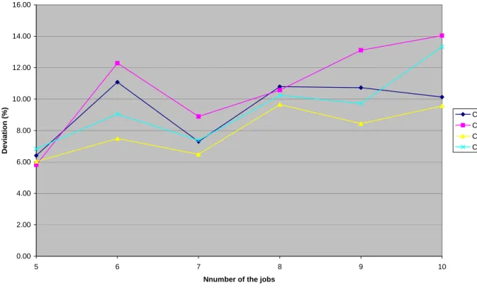
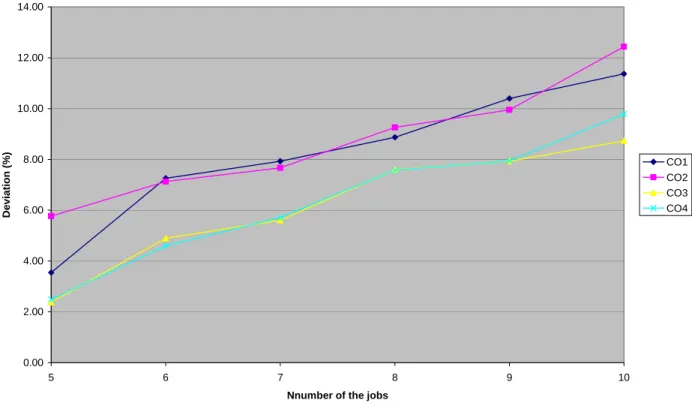
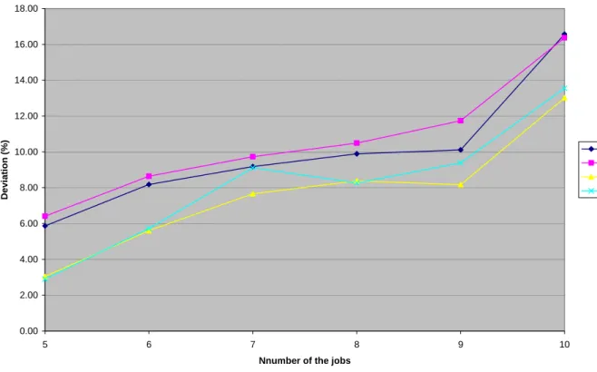
Figure 1 through Figure 6 summarize the computational results for the 1440 test problems, differentiated according to the m and TF values. Figure 1 depicts the curves representing the variation of the percentage of average deviation error of four algorithms, namely CO1 through CO4, from the optimal solution for the values of m=5 and TF=0.1 and according to the variation of number of the job (n=5through 10). Figure 2 through Figure 6 depict similar type of curves for the given pair values of (m=5 and TF=0.2),(m=5and TF=0.4),(m=8and TF-0.1), (m=8and TF=0.2), and (m=8 and TF=0.4) respectively. These figures reveal that in most cases, algorithm CO3
performs better than other three algorithms, while algorithm CO4 performs almost as well as algorithm CO3.
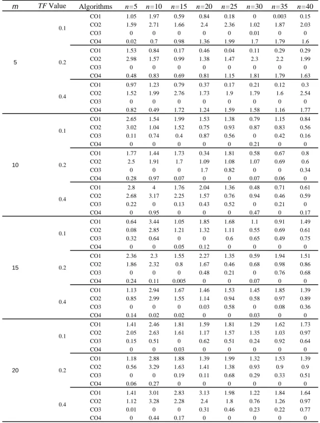
For evaluating the relative effectiveness of the developed algorithms, we generated 4060 larger sized test problems. For a scenario defined by any given values of m, n, and TF, we generated 40 different test problems. In each scenario, all 40 test-problems are solved by four developed algorithms and their associated total tardiness values are determined. Then we calculated the average of the total tardiness for 40 test problems of each scenario. To define the relative effectiveness, we designated the index solution by selecting the minimum total tardiness which is obtained by one of the developed algorithms, and determined the relative effectiveness of each algorithm through the following formula.
100
}
{
min
}
{
min
×
−
=
k k
k k
i i
ATT
ATT
ATT
RAD
Where ATTi is the average total tardiness of the 40 test problems (in one scenario) solved by the i th algorithm,
min
{
k}
k
ATT
is the value of the index solution, and RADiis the percentage of the average deviation of the ith algorithm. We then defined 96 different scenarios by assigning eight different values to n (n=5, n=10, n=15, n=20, n=25, n=30, n=35, n=40), four different values to m (m=5, m=10, m=15, m=20), and three different values to TF (TF=0.1, TF=0.2, TF=0.4). For each scenario 40 test problems are generated and solved by the developed algorithms and their relative average deviations are calculated. Table 1 demonstrates the values of the percentage average deviation of each scenario obtained by each algorithm. This table reveals that algorithm CO3 performs better than others for smaller sized problems and algorithm CO4 performs better than others for larger sized problems.6. CONCLUSION
In this paper we considered the generalized tardiness flow shop scheduling model with the total tardiness as its measure of performance. We modified the COVERT index, and employed this index as a sequencing rule for developing four algorithms.
To evaluate the effectiveness of the algorithms, we used the concept of pseudo random number generation for generating a set of test problems. For different values of the input parameters, such as the number of jobs, the number of machines, and the values of due date tightness parameter, we defined a set of scenarios for generating the test problems. For each scenario, 40 randomly generated test problems were generated and solved to determine the effectiveness of the proposed algorithms in obtaining the optimal solution. As the result, it was shown that both CO3 and CO4 algorithms can provide solutions with the average deviation of less than 8% from the optimal solutions with very little computational effort. This is due to the fact that each algorithm enumerates only m different schedules for providing the final solution. The result of the computational experiments, for evaluating the relative effectiveness of the algorithms, revealed that both CO3 and CO4 had better performance compared to the other two. It was also revealed that, CO3 performed better for smaller sized problem, while CO4 performed better as the problem size becames larger.
0.00 2.00 4.00 6.00 8.00 10.00 12.00 14.00 16.00
5 6 7 8 9 10
Nnumber of the jobs
Deviat
io
n (
%
)
CO1 CO2 CO3 CO4
Figure 1. Deviation of the total tardiness obtained by algorithms from the optimal solution (m=5, TF=0.1)
0.00 2.00 4.00 6.00 8.00 10.00 12.00 14.00
5 6 7 8 9 10
Nnumber of the jobs
Deviat
io
n (
%
)
CO1 CO2 CO3 CO4
0.00 2.00 4.00 6.00 8.00 10.00 12.00 14.00
5 6 7 8 9 10
Nnumber of the jobs
D
eviat
io
n (
%
)
CO1 CO2 CO3 CO4
Figure 3. Deviation of the total tardiness obtained by algorithms from the optimal solution (m=5, TF=0.4)
0.00 2.00 4.00 6.00 8.00 10.00 12.00 14.00 16.00 18.00
5 6 7 8 9 10
Nnumber of the jobs
D
evi
at
io
n
(
%
)
CO1 CO2 CO3 CO4
0.00 2.00 4.00 6.00 8.00 10.00 12.00 14.00 16.00 18.00
5 6 7 8 9 10
Nnumber of the jobs
Deviat
io
n (
%
)
CO1 CO2 CO3 CO4
Figure 5. Deviation of the total tardiness obtained by algorithms from the optimal solution (m=8, TF=0.2)
0.00 2.00 4.00 6.00 8.00 10.00 12.00
5 6 7 8 9 10
Nnumber of the jobs
Deviat
io
n (
%
)
CO1 CO2 CO3 CO4
Table 1. Relative deviation (%) of the TT obtained by each algorithm from the best among them.
m TF Value Algorithms n=5 n=10 n=15 n=20 n=25 n=30 n=35 n=40
5
0.1
CO1 1.05 1.97 0.59 0.84 0.18 0 0.003 0.15 CO2 1.59 2.71 1.66 2.4 2.36 1.02 1.87 2.03
CO3 0 0 0 0 0 0.01 0 0
CO4 0.02 0.7 0.98 1.36 1.99 1.7 1.79 1.6
0.2
CO1 1.53 0.84 0.17 0.46 0.04 0.11 0.29 0.29 CO2 2.98 1.57 0.99 1.38 1.47 2.3 2.2 1.99
CO3 0 0 0 0 0 0 0 0
CO4 0.48 0.83 0.69 0.81 1.15 1.81 1.79 1.63
0.4
CO1 0.97 1.23 0.79 0.37 0.17 0.21 0.12 0.3 CO2 1.52 1.99 2.76 1.73 1.9 1.79 1.6 2.54
CO3 0 0 0 0 0 0 0 0
CO4 0.82 0.49 1.72 1.24 1.59 1.58 1.16 1.77
10
0.1
CO1 2.65 1.54 1.99 1.53 1.38 0.79 1.15 0.84 CO2 3.02 1.04 1.52 0.75 0.93 0.87 0.83 0.56 CO3 0.11 0.74 0.4 0.87 0.56 0 0.42 0.16
CO4 0 0 0 0 0 0.21 0 0
0.2
CO1 1.77 1.44 1.73 0.34 1.81 0.58 0.67 0.8 CO2 2.5 1.91 1.7 1.09 1.08 1.07 0.69 0.6
CO3 0 0 0 1.7 0.82 0 0 0.34
CO4 0.28 0.97 0.07 0 0 0.07 0.06 0
0.4
CO1 2.8 4 1.76 2.04 1.36 0.48 0.71 0.61 CO2 2.68 3.17 2.25 1.57 0.76 0.94 0.46 0.59 CO3 0.22 0 0.13 0.43 0.52 0 0.21 0
CO4 0 0.95 0 0 0 0.47 0 0.17
15
0.1
CO1 0.64 3.44 1.05 1.85 1.68 1.1 0.91 1.49 CO2 0.08 2.85 1.21 1.32 1.11 0.55 0.69 0.61 CO3 0.32 0.64 0 0 0.6 0.65 0.49 0.75
CO4 0 0 0.05 0.12 0 0 0 0
0.2
CO1 2.36 2.3 1.55 2.27 1.35 0.59 1.94 1.51 CO2 1.86 2.32 0.8 1.67 0.46 0.68 0.98 0.86 CO3 0 0 0 0.48 0.21 0 0.76 0.68 CO4 0.24 0.11 0.005 0 0 0.07 0 0
0.4
CO1 1.13 2.94 1.67 1.46 1.53 1.45 1.85 1.39 CO2 0.85 2.99 1.55 1.14 0.94 0.58 0.97 0.89 CO3 0 0 0 0.03 0.58 0 0.08 0.36 CO4 0.14 0.02 0.02 0 0 0.03 0 0
20
0.1
CO1 1.41 2.46 1.81 1.59 1.81 1.29 1.62 1.73 CO2 2.05 2.63 1.61 1.17 1.57 1.35 1.03 0.97 CO3 0.15 0.51 0 0.62 0.51 0.24 0.92 0.64
CO4 0 0 0.03 0 0 0 0 0
0.2
CO1 1.18 2.88 1.88 1.39 1.99 1.32 1.53 1.39 CO2 0.56 3.29 1.63 1.41 1.38 0.93 0.9 0.9 CO3 0 0 0.19 0.11 0.68 0.29 0.33 0.51
CO4 0.06 0.27 0 0 0 0 0 0
0.4
CO1 1.41 3.01 2.83 3.13 1.98 1.22 1.84 1.64 CO2 1.12 3.28 2.28 2.4 1.8 0.76 1.26 0.97 CO3 0.01 0 0 0.31 0.46 0.23 0.22 0.77
REFERENCES
[1] Ahmadi J.H., Ahmadi R.H., Dasu S., Tang C.S. (1992), Batching and scheduling jobs on batch and discrete processors; Operations Research 40(4); 750-763.
[2] Allahverdi A., Al-Anzi F.S. (2002), Using two-machine flow shop with maximum lateness objective to model multimedia data objects scheduling problem for WWW applications; Computers and Operations Research 29(8); 971-994.
[3] Armentano V.A., Ronconi D.P. (1999), Tabu search for total tardiness minimization in flow shop scheduling problems; Computers & Operations Research 26(3); 219-235.
[4] Baker K.R. (1974), Introduction to Sequencing and Scheduling; John Wiley & Sons Inc., New York. [5] Baker K.R. (1984), Sequencing rules and due date assignments in a job shop; Management Science
30(9); 1093-1104.
[6] Baker K.R., Schrage L.E. (1987), Finding an optimal sequence by dynamic programming: an extension to precedence-related tasks; Operations Research 26; 111-120.
[7] Baker K.R., Schrage L.E. (1990), Sequencing with earliness and tardiness penalties: a review; Operations Research 38; 22-36.
[8] Bilge U., Kirac F., Kurtulan M., Pekgun P. (2004), A Tabu search algorithm for parallel machine total tardiness problem; Computers & Operations Research 31(3); 397-414.
[9] Carroll D.C. (1965), Heuristic sequencing of jobs with single and multiple components; Ph.D. Dissertation, Sloan School of Management, MIT, Mass.
[10] Etiler O., Toklu B., Atak M., Wilson J. (2004), A generic algorithm for flow shop scheduling problems; Journal of Operations Research Society 55(8); 830-835.
[11] Faaland B., Schmitt T. (1987), Scheduling tasks with due dates in a fabrication/assembly process; Operations Research 35(3); 378–388.
[12] Ghassemi-Tari F., Olfat L. (2004), Two COVERT based algorithms for solving the generalized flow shop problems; Proceedings of the 34th International Conference on Computers and Industrial Engineering 34; 29-37.
[13] Ghassemi-Tari F., Olfat L. (2007), Development of a set of algorithms for the multi-projects scheduling problems; Journal of Industrial and Systems Engineering 1(1); 11-17.
[14] Glover F. (1994), Tabu search fundamentals and uses; Working paper; University of Colorado, Colorado.
[15] Hall N.G., Posner M.E. (1991), Earliness-tardiness scheduling problems, I: Weighted deviation of completion times about common due date; Operations Research 39; 836-846.
[16] Hall N.G., Posner M.E. (1991), Earliness-tardiness scheduling problems, II: Deviation of completion time about common due date; Operations Research 39; 847-856.
[17] Hall N.G., Posner M.E. (2001), Generating experimental data for computational testing with machine scheduling applications; Operations Research 49; 854-865.
[18] Kanet J. (1981), Minimizing the average deviation of job completion times about a common due date; Naval Research Logistics Quart. 28; 643-651.
[19] Karimi A. (1992), Optimal cycle times in multistage serial systems with set-up and inventory costs; Management Science 38(10); 1467–1481.
[20] Kim Y.D. (1993), Heuristics for flow shop scheduling problems minimizing mean tardiness; Journal of Operations ResearchSoc. 44(1); 19-28.
[21] Lauff V., Werner F. (2004), On the complexity and some properties of multi-stage scheduling problems with earliness and tardiness penalties; Computers & Operations Research 31(3); 317-345. [22] Lee I. (2001), Artificial intelligence search methods for multi-machine two-stage scheduling with due
date penalty, inventory, and machining costs; Computers & Operations Research 28(9); 835-852. [23] Mosheiov G. (2003), Scheduling unit processing time jobs on an m-machine flow shop; Journal of the
Operations Research Society 54(4); 437-441.
[24] Rachamaduagu R.V., Morton T.E. (1982), Myopic heuristic for the single machine weighted tardiness problem; Working paper Gs. IA, Carnage Mellon University 38; 82-83.
[25] Rachamaduagu R.V. (1984), Myopic heuristic in open shop scheduling; Proceedings of the 14 Annual Pittsburgh Conference on Modeling & Simulation; 14; 1245-1250.
[26] Sapar H., Henry M.C. (1996), Combinatorial evaluation of six dispatching rules in dynamic two-machine flow shop; International Journal of Management Science 24(1); 73-81.
[27] Suliman S.M.A. (2000), A two-phase heuristic approach to the permutation flow shop scheduling problem; International Journal of Production Economics 64(1-3); 143-152.
[28] Sundararaghavan P., Ahmed A.U. (1984), Minimizing the sum of absolute lateness in single-machine and multi-machine scheduling; Naval Research Logistics Quart 31; 325-333.
[29] Vepsalainen A.P.J., Morton T.E. (1987), Priority rules for job shops with weighted tardiness costs; Management Science 23(8); 1035-1047.
[30] Yeh W., Allahverdi A. (2004), A branch and bound algorithm for the three machine flow shop scheduling problem with bi-criteria of make-span and total flow time; International Transaction in Operations Research 11(30); 323-327.