1
The impact of EU carbon price changes on the stock performance of European electricity firms
By
John Townsend Schmale
Honors Thesis
Economics Department
University of North Carolina
March 31, 2014
Approved:
______________________________
2
Abstract
3
I. Introduction
There have been considerable international policy efforts over the last twenty years to
mitigate carbon dioxide (CO2) emissions, the most notable coming in 1997 with the Kyoto
Protocol—an international agreement linked to the United Nations Framework Convention on
Climate Change. The Kyoto Protocol commits its parties to reduce their greenhouse gas
emissions by 8% of the 1990 level over the 2008 to 2012 period. EU authorities are responsible
for making sure this overall cap on total emissions from all sectors of the economy in all 28 EU
countries along with Iceland, Liechtenstein, and Norway is met. The European Union Emission
Trading Scheme (EU ETS) is one mechanism used to help meet this goal. The scheme is a ‘cap
and trade’ market-based approach to mitigate carbon emissions, allowing firms the flexibility to
abide by the scheme in the most cost-effective way, buying and selling carbon permits, called
European Union Allowances (EUAs), as needed. Each EUA gives its holder the right to emit one
ton of carbon dioxide. More than 11,000 power stations and manufacturing plants, around 45%
of total EU emissions, are limited by the EU ETS. The firms limited by the EU ETS are labeled
as part of the “trading sector” and include those industries which are the largest emitters of
carbon dioxide: electricity production, oil refining, heating and gas transportation along with
major emitters in the industrial sector. Under the scheme, firms are allocated permits based on
historical emission levels and then can trade these permits in the marketplace. At the end of each
year every firm regulated by the scheme is responsible for owning enough allowances to cover
their emissions for the past year. If all emissions are not accounted for with the appropriate
amount of permits, a fine is administered per ton of CO2 short.
The EU ETS is a decentralized cap and trade model with each country devising its own
4
emissions budget is allocated to the “trading” and “non-trading sectors”, and how stringent the
permit allocation process will be (Kruger et al., 2007). Countries such as Spain, Italy, and the
UK have the most stringent caps meaning that firms in these countries are more likely to be
allocated a smaller percentage of permits in relation to their observed emissions (Bushnell et al.,
2012).
Phase I of the EU ETS began in 2005 and operated as a pilot period for every participant
involved to get used to the scheme before the Kyoto binding Phase II period began in 2008. The
transition to Phase II saw the share of free allocation of allowances decrease from 95% to 90%
and the penalty for not having enough permits become much greater, increasing from 40€ per ton
to 100€ per ton (Mo et al. 2012). The EU ETS started as and still is the largest international
greenhouse gas (GHG) emission allowance market. The annual value of permits consumed in the
market reached nearly €60 billion in 2012 (Bushnell et al., 2012). A sufficiently high carbon
price should lead firms to shift generation to lower emitting plants and promote investment in
clean, low-carbon technologies. Along with being a mechanism to help achieve the commitments
required by the Kyoto Protocol, the design of the EU ETS is such that by 2020, the end of Phase
III (2013-2020), carbon emissions from the sectors covered will be 21% lower than 2005 levels
(EC Climate Action, 2013).
The implementation of this new regulation led to research investigating the potential
economic consequences. Subjects of interest include how the EU ETS has impacted firms’
profitability, investment decisions, and competition with other firms and industries along with
what the optimal level of auctioning should be, what the optimal design of a country’s National
Allocation Plan should be, and whether the EU ETS is a cost-effective model.1 Understanding
1
5
the economic impacts of the EU ETS is not only important for having a better grasp on potential
consequences in Europe, but for helping better design future carbon cap and trade systems in
other parts of the world as well. One area of economic interest related to the EU ETS has been
the financial market impact EUA price developments have had on the stock performance of
firms. Several papers have specifically looked at the relationship between changes in EUA prices
and the stock performance of European electricity firms, Oberndorfer (2009) and Mo et al.
(2012). The electricity sector is the largest single source of emissions in the scheme, accounting
for 57%, and will have to obtain the most permits, thus this sector is of great interest for research
centered on the impacts of the EU ETS (Bushnell et al., 2012).
Fundamental market valuation assumes that capital markets will value a firm at its
expected discounted future profits. Looking at the relationship between changes in EUA prices
and stock performance provides a lens to see how investors believe firms’ profits are affected by
EUA prices. A decrease in EUA prices is equivalent to a relaxation of regulation. The structure
of the scheme is such that most of the permits needed by firms, 95% in Phase I and 90% in Phase
II, were grandfathered in, meaning they were allocated to firms freely based on historical
emission levels. The initial permit net short / long position of a firm varied, depending on the
country and industry it is a part of. The net position of a firm is significant in determining the
impact the scheme has on profit. If a firm is in a net short position and the price of EUAs rises
then this indicates an increase in compliance costs which could lead to a decrease in future
profits. If a firm is in a net long position and the price of EUAs rises then this indicates an
increase in potential revenue from selling the unneeded permits in the market at the now higher
price, which would lead to an increase in future profits. The concept of windfall profits has been
6
allowing them to profit from the regulation. Another important factor to consider is the cost
pass-through ability of the firm. Most EU member states were very explicit that the expected shortage
of EUAs was to be assigned to the electricity sector because of the limited competition present in
this sector along with the relatively inelastic demand for electricity (Ellerman et al., 2007). This
would allow firms in this sector to more easily pass on EU ETS compliance costs to consumers
through higher prices, which increases revenue, and possibly leaves profits largely unchanged by
the increased costs and revenues balancing out. With a high enough EUA price, firms will also
face the business decision of whether it would be more cost effective to switch to cleaner power
generating methods, possibly from coal to natural gas. This investment decision would be
associated with new fixed costs but lower EU ETS marginal compliance costs.
Following capital market theory, if there is a negative correlation between EUA price
increases and stock performance of European electricity firms it can be assumed that when EUA
prices increase, the expected future profits of the firm decrease. If there is a positive correlation it
can be assumed that an increase in regulation leads to an increase in profit for European
electricity firms. A correlation of zero would indicate that capital markets either believe the
scheme changes the costs and revenues of the firm in such a way that the two balance out and
profits remain unchanged or that the costs or revenue associated with the scheme are so
negligible that they aren’t taken into account when estimating future profits.
This paper will fill the current literature gap on the relationship between EUA price
changes and the stock value of European electricity firms. To my knowledge, there have been no
studies on this subject that look further than 2009, which is only two years into Phase II of the
scheme. For my analysis, I use the model from the research conducted by Mo, Zhu, and Fan
7
general a positive correlation during Phase I, and the research specifically by Mo, et al. (2012)
found a negative relationship to exist in the first two years of Phase II. Mo et al. (2012) also
identified that the relationship between changes in EUA prices and stock performance varied
significantly from one firm to the next.
There are two prevailing forces that I expect will influence the profitability of firms and
thus my results during my period of interest, 2010-2012. I expect a downward pressure on
correlation to be exerted from an increase in regulation stringency as the scheme continues to
lower its cap and lower the amount of permits grandfathered in. I also expect an upward pressure
to come from the fact that Europe, like most of the rest of the world, was dealing with a
recession during this time period, leading to a decrease in demand for electricity which means
less output and less emissions from electricity firms. If a firm’s emissions totals are less than
what was forecasted, a higher percentage of needed permits will be covered by those
grandfathered to the firm, cutting compliance costs. Knowing that a surplus of permits has been a
big concern related to the EU ETS, with the European Commission reporting that by the end of
Phase II the surplus stood at almost two billion allowances, I believe this upward pressure on
profits will outweigh the downward pressure of increased regulatory stringency (EC Climate
Action, 2013). I expect the relationship between EUA price changes and stock performance of
European electricity firms to be more positively correlated than the literature has shown it to be
over the earlier time period.I expect that there will be country-specific stock market effects
given the decentralized nature of the EU ETS, with firms in countries with more stringent
allocation policies having lower carbon price coefficients, possibly even negative. I also expect
8
to either have a positive correlation for the entirety of the phase or a negative one for the entirety
of the phase.
II. Literature Review
This section will contain a discussion of previous literature that examined the financial
market effects the EU ETS has on European electricity firms. The first econometric analysis on
the stock market effects of the EU ETS was completed by Oberndorfer (2009). He used a
multifactor market model to test the relationship between EUA price changes and the stock
market return of 12 European electricity corporations, which included Aem (Italy — IT), British
Energy Group (United Kingdom—UK), Eon (Germany—DE), Endesa (Spain—ES), Enel (IT),
Energias de Portugal (Portugal), Fortum (Finland), Iberdrola (ES), International Power (UK),
RWE (DE), Scottish & Southern Energy (UK), and Union Fenosa (ES). He included the market
return, oil price changes, electricity price changes, and gas price changes as control variables in
his model. The data used in the analysis spans from 2005 through 2007. He used a multitude of
regression methods, including an ordinary least squares (OLS) process using an equal-weighted
portfolio approach and a panel approach, as well as a Generalized AutoRegressive Conditional
Heteroskedasticity (GARCH) model. These frameworks are augmented by including
country-specific indicator variables in order to take into account country-country-specific stock market effects to
EUA price developments. Interaction terms to take into account possible asymmetries were
included as well to allow the model to be able to identify whether an increase in EUA prices had
a different magnitude of effect on returns than an equal decrease in EUA prices. EUA settlement
price changes were used, and Oberndorfer noted that although futures prices are less affected by
9
because of the thin trading volume in the futures market during his period of analysis. Electricity
prices from the German market were used as a proxy for overall EU electricity prices.
His results show a positive correlation between changes in EUA prices and stock
performance of European electricity firms. The estimated carbon price beta estimate varies
between regression models from 0.001 and 0.002, indicating that as EUA prices increase, the
firms’ stock value rises as well. Oberndorfer did not find evidence for an asymmetric reaction of
electricity stock returns to EUA price changes. He did find though that the EUA effect on the
stock market is country-specific with Spanish electricity firms exhibiting a slightly negative
relationship and all other countries exhibiting a positive relationship, with UK firms having the
most positive relationship.
In related research on the financial market effects of the EU ETS, Mo, Zhu, and Fan
(2012) used a slightly different CAPM style model and regression method than Oberndorfer.
They differ from Oberndorfer by excluding changes in gas prices as a control variable and by
using futures prices from the IntercontinentalExchange (ICE) instead of spot prices from the
European Energy Exchange (EEX). Mo, et al. accounts for the issues of thin initial trading
volume in the EUA futures market by using a regression technique which implements lead and
lag terms. The authors also looked at the relationship in a much more disaggregated manner than
Oberndorfer. They ran separate regressions for each electricity firm to be able to see the
relationship on a firm-specific level. They also ran separate regressions for each year of data
spanning from 2006 through 2009 to investigate whether the relationship changed over time as
the EU ETS evolved, moving from Phase I to Phase II. Like Oberndorfer, the authors looked at
10
(FR), Endesa (ES), Enel (IT), Fortum (FI), Iberdrola (ES), International Power (UK), Public
Power Corporation (GR), Red Eléctrica de España (ES), Scottish & Southern Energy (UK),
Terna Group (IT). To look at the results in a more generalized fashion they took the mean and
median of their results.
Results indicated that the effect of a change in EUA prices on European electricity firm
returns varied significantly from firm to firm. When aggregated, the beta coefficient for EUA
price changes had a mean of -0.014 and a median of -0.002. For Phase I, the mean was 0.006 and
for Phase II the mean was -0.0334. These results suggest that the increase in regulation
stringency in Phase II caused an increase in EUA prices to lead to depreciation in corporate value
instead of appreciation in value like it had done in Phase I. The higher absolute value also
indicated that firms had a higher sensitivity to EUA price changes in Phase II.
Research by Bushnell, Chong, and Mansur (2012) investigated the ways in which firms
can profit from regulation, specifically looking at the implementation of the EU ETS. New
regulation impacts both costs and revenues in a multitude of ways causing the profitability
puzzle to be complex. This research took an event study approach, investigating the potential for
abnormal returns on firms contained in the Dow Jones STOXX 600 index in late April 2006
when there was a sharp devaluation of EUA prices. The authors provide a theoretical model
which considered the factors of firm profitability that changes in EUA prices could impact. The
model included consumer demand, the cost of producing electricity, the value of EUAs in
possession, the cost of compliance, and the cost of abatement. The model is intended to be
general, encompassing both perfectly competitive industries and those in which individual firms
11
Results showed that the sharp devaluation in EUA prices impacted sectors differentially,
and that the sectors that emit the most CO2 performed the worst during the event. The authors
believed this indicates that the higher emitting sectors, which the electricity sector is a part of,
are able to profit from the regulation associated with the EU ETS. The authors also noted that the
results of their study indicate that equity markets are strongly focused on revenue effects
associated with EUA prices.
III. Empirical Framework
My research uses a multifactor model in accordance with Mo et al. (2012). The factors
used in this model to explain the stock performance of European electricity firms are the market
return, changes in electricity prices, changes in oil prices, and the factor of primary interest,
changes in EUA prices. The market return is included because as suggested by the Capital Asset
Pricing Model (CAPM), the risk-to-reward ratio of any security in relation to that of the overall
market is the decisive factor for the pricing of the individual security. Previous literature
concludes that oil is one of the main indicators for energy-price developments as a whole, and so
oil price changes are included as a control variable here (Oberndorfer, 2009). Electricity price
changes are included because electricity is the main product of the companies we are analyzing.
Mo et al. (2012) cited previous literature that had shown there to be a significant relationship
between the stock returns of a firm and the price of the firm’s main product. EUA price changes
are included because the relationship between EUA prices and the value of European electricity
companies is the main focus of this research. Like Mo et al. (2012), I analyze the stock returns of
these corporations in disaggregated form allowing the identification of firm-specific EUA
effects. Daily data was used to estimate OLS regressions. Infrequent or thin trading, which was
12
estimates (Sercu, 2007). To alleviate this problem, the authors incorporated lead and lag terms
for the independent variables and I do this as well. The result is a multifactor market model
which can be expressed as follows:
( )
where ϵi,t is a disturbance term with E(єi,t)=0 and var(єi,t)=σ2 and is a constant. is
the stock market return of the individual European electricity firms. , , , and
are the lag terms for market return, electricity price changes, oil price changes, and carbon
price changes respectively. , , , and are the synchronous terms for market return,
electricity price changes, oil price changes, and carbon price changes respectively. ,
, , and are the lead terms for market return, electricity price changes, oil price
changes, and carbon price changes respectively. The βs are the OLS estimates of the coefficients
on the variables in the model. The aggregate coefficient estimates are calculated by adding the
lag, synchronous, and lead beta estimates for each variable:
A positive value of β indicates that the variable has a positive correlation with the stock
performance of the firm. The model is estimated for each European electricity firm in one year
blocks. The mean and median of the individual companies’ β series were calculated to obtain an
13
the research to the new time period of interest, 2010-2012. In total I will run 84 (12 firms*7
years) individual regressions.
I will also run a slightly modified model of Mo, et al. (2012), which will include three
additional European electricity firms CEZ Group (Czech Republic--CZ), E.ON (Germany—DE),
and RWE (DE). I include these three because they all have significant market share in the
European electricity sector (Convery, 2007). The two German electricity firms were also added
because there were no German firms represented in the study by Mo et al., which appears to be a
serious omission given that Germany firms were awarded roughly half the total EU cap in
permits (Convery, 2007). I will no longer include lead and lag terms in the model either as the
trading volume significantly increases during Phase II of the scheme (see Figure 1). Another
alteration from the original model is that I will be running the regressions by phase not in yearly
blocks. By running it in phases I am expecting to provide a better comparison of overall trends
between Phase I and Phase II. In total I will have 30 (15 firms*2 phases) individual regressions
for this supplemental analysis.
Figure 1
*EU Allowances are traded in lots of 1000
0 200 400 600 800 1000 1200 Jan -06 Ju n -06 N o v-06 Ap r-07 Se p -07 Fe b -08 Ju l-08 De c-0 8 Ma y-0 9 Oct-09 Ma r-10 Au g-10 Jan -11 Ju n -11 N o v-11 Ap r-12 Se p -12 m ill io n to n s CO 2
EUA Monthly Trading Volume
Phase I
14
IV. Data
I first looked at the same 12 electricity firms that Mo et al. (2012) used for their study:
a2a (IT), Drax Group (UK), Électricité de France (FR), Endesa (ES), Enel (IT), Fortum (FI),
Iberdrola (ES), International Power (UK), Public Power Corporation (GR), Red Eléctrica de
España (ES), Scottish & Southern Energy (UK), Terna Group (IT). The daily stock price data
was taken from Reuter’s DATASTREAM service and the adjusted price was used for the series.
The data series used for the market return was the STOXX Europe 600 Utilities Index, which
was also retrieved from DATASTREAM. The data series used for changes in oil prices was the
Europe Brent Spot Price (FOB) retrieved from the U.S. Energy Information Administration.
Brent is the most relevant traded crude for European energy firms (Oberndorfer 2009). No
common market for electricity exists in the EU, but the prevailing literature has used German
electricity prices from the European Energy Exchange (EEX) as a proxy. Germany is the biggest
electricity market in Europe and the EXX is one of the most liquid European power exchanges.
Unable to obtain the electricity contract used by Mo et al. in their research, I used the German
electricity futures Phelix month base series from the EEX, the same series that Oberndorfer
(2009) used. For this data series I used the prices of contracts that were one month away from
expiration. As the explanatory variable of primary interest, the EUA data series was retrieved
from the IntercontinentalExchange (ICE). The daily prices of EUA futures contracts that were to
expire at the end of the current year were used. EUA prices have developed very similarly in all
marketplaces so the choice of marketplace is not of major concern (Oberndorfer, 2009). The
15
V. Results
The market model was estimated for each sample company from 2006-2012 (details in
Table A found in the Appendix section). The aggregate results from the previous literature are
compared with those from mine during the 2006-2009 time period in Table 1 and 2.
The mean for Βm was 0.091 smaller in my analysis compared to the prior study, the mean for Βe
was 0.070 smaller, the mean for Βo was .005 larger, and the Βc was 0.011 larger. Overall, the
results seem to indicate that my model and data replicated the previous study fairly well. The
only factor which had a coefficient with a different sign than the previous study was changes in
electricity prices. Although it is surprising that the relationship changed from being positively
correlated to now slightly negative, the fact that the data series I used for electricity prices was
different than the one used in Mo et al.’s analysis explains why variation could exist. It is no
surprise that the market beta is by far the most significant factor in the model. The mean βm value
of 0.810 indicates that an increase in the market return of 10% would lead to an increase in the
stock return of these firms by 8.1% on average. The βc value of -0.003 indicates that a change in
EUA prices of 10% leads to a 0.03% decrease in stock performance of European electricity firms
Table 1
Mean and median β estimates from Mo et al. (2012) for 48 firm-year observations (12 firms*4 years)
βm (market beta)
βe (electricity price effect)
βo (oil price effect)
βc (EUA price effect)
Mo, et al.Mean (2006-2009) 0.901 0.068 0.042 -0.014
Mo, et al.Median (2006-2009) 0.870 0.058 0.016 -0.021
Table 2
Mean and median β estimates for 48 firm-year observations (12 firms*4 years)
βm (market beta)
βe (electricity price effect)
βo (oil price effect)
βc (EUA price effect)
Mean (2006-2009) 0.810 -0.002 0.047 -0.003
16
on average over this period. This is a very small amount indicating that capital markets view the
EU ETS as not shrinking the firms’ profits very much on average during this time period. But it
is important to keep in mind that the carbon price beta estimates did vary greatly from firm to
firm, ranging from -0.232 to 0.244.
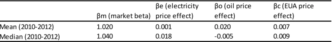
The mean and median results from when the study is extended to the new time period of
interest are presented in Table 3.
The mean for Βm was 0.210 bigger during the 2010-2012 interval compared to my results from
the 2006-2009 period, for Βe the mean was 0.003 bigger, for Βo it was -0.027 smaller, and for Βc
it was 0.010 bigger. One explanation for why the carbon price beta might have switched from
negative to positive is that the electricity firms might have found themselves more often in a net
long position in terms of permits in the 2010-2012 time range, which wouldn’t be surprising
given the surplus of permits in the market. If a firm is in a net long position and the price of
EUAs increases, expected future profits will increase as the firm can sell the unneeded permits
on the market for a greater amount of revenue. Greater future profits translate into appreciation
of stock value. The absolute value is still fairly small, with a 10% increase in EUA prices leading
to a .07% increase in stock return on average. This indicates that the capital markets continue to
believe the EU ETS does not affect the profits of European electricity firms too significantly.
Figure 2 provides a visual of the change in carbon price beta for each firm individually over the
entire 2006-2012 period.
Table 3
Mean and median β estimates for 36 firm-year observations (12 firms*3 years)
βm (market beta)
βe (electricity price effect)
βo (oil price effect)
βc (EUA price effect)
Mean (2010-2012) 1.020 0.001 0.020 0.007
17
Figure 2
The development of βc from 2006 to 2012 for each firm
As one can see, the variation in the carbon price beta estimates not only varies from one firm to
another but varies in an individual firm significantly over time as well. As an example, Public
Power Corporation has a carbon price beta of 0.244 in 2008 which changes to -0.278 in 2010.
One element of the graph that stands out is the 2007 to 2008 region. The carbon price betas
across all firms in 2007 can be characterized by having a value extremely close to zero. One
major reason for changes in the price of EUAs having relatively no impact during this year was
the banking policy of the EU ETS that did not allow the usage of permits obtained in Phase I to
be used in Phase II. EUA prices consistently fell (see Figure 3 below) once the market became
aware that there was a surplus present and that the permits were without value when Phase I
ended at the end of 2007 (Convery, 2007). Even if changes in EUA prices are large on a
percentage basis, the impact the change will have on profits is small if the price of the permits
are close to zero like they were for most of 2007. The carbon price beta estimates in 2008 are
characterized by a large deviation from the 2007 levels for all firms, some becoming positively
B
ETA
18
correlated, some negatively. This dispersion away from zero can be explained by the price of the
permits re-entering the €20-€30 range. For the new period of interest, 2010-2012, there does not
seem to be present much of a trend at all on the individual firm level. Some firms’ stock value
maintain the same type of relationship across all three years while others switch from being
positively correlated to negatively correlated or vice versa. This was not consistent with my
hypothesis. It appears firms did not establish themselves in the eyes of the capital markets as
either being consistently hurt or helped by the scheme during Phase II.
Figure 3
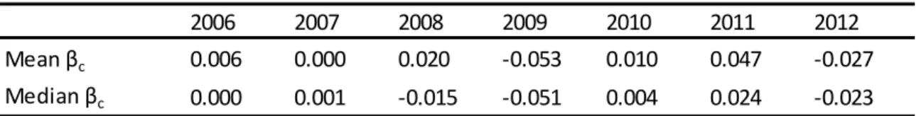
Table 4 presents a summary of the development of the carbon price beta estimates over
time on a year by year basis.
The fluctuation back and forth between a positive and negative mean for carbon price beta
estimates in Phase II is surprising. Again, I would have expected a common trend to have 0
5 10 15 20 25 30 35
€
/to
n
o
f CO
2
EUA DAILY PRICE
Phase I
Phase II
Table 4
Development of βc over time by year
2006 2007 2008 2009 2010 2011 2012
Mean βc 0.006 0.000 0.020 -0.053 0.010 0.047 -0.027
19
established of whether capital markets believe the scheme affects firms’ profits positively or
negatively.No misspecification tests were completed because the intent of this study was to use
the exact same model as that used in Mo et al.’s research.
The supplemental analysis I conducted added three additional firms: CEZ Group (CZ),
E.ON (DE), and RWE (DE). The regressions were conducted not in yearly blocks but by the two
phases (details in Table B found in the Appendix section). The aggregate results are presented in
Table 5 and Table 6.
The results indicate that the mean market beta estimates increased by .104 from Phase I to Phase
II, the mean electricity price beta estimates decreased by .023, the mean oil price beta estimates
decreased by .006, and the EUA price beta estimates increased by .022. The electricity price beta
estimates are surprising. It doesn’t seem very reasonable to assume an increase in electricity
prices, the source of revenue for these firms, would signal a drop in firm value. The market beta
estimates and oil price beta estimates stay fairly consistent from Phase I to Phase II—changing
by 15.5% and 20.7% respectively. This makes sense as the only relationship that should be
significantly altered by the changes in regulations associated with the EU ETS is the carbon price
*Table 5
Mean and median estimates for 15 firms during Phase I βm (market beta)
βe (electricity price effect)
βo (oil price effect)
βc (EUA price effect)
Phase I Mean 0.671 0.008 0.029 0.000
Phase I Median 0.635 0.005 0.007 0.000
*Phas e I of the EU ETS began i n 2005, but thi s s tudy onl y l ooks at data s tarti ng i n 2006
Table 6
Mean and median estimates for 15 firms during Phase II βm (market beta)
βe (electricity price effect)
βo (oil price effect)
βc (EUA price effect)
Phase II Mean 0.775 -0.015 0.023 0.022
20
beta estimate. Given that Oberndorfer (2009) had found the estimated carbon price beta on
average for Phase I to be between 0.001 and 0.002 and that Mo et al. (2012) had found it be
0.0055, I was surprised to see my results have a Phase I mean βc value very close to zero at
0.000. One explanation could be that I used a different mix of firms for my analysis than either
prior study. Another explanation of why my results differed from Mo et al. (2012) in particular
could be from my model not including lead and lag terms in this supplementary analysis. The
value of 0.000 on its own is not surprising to me though, as it was the pilot phase with 95% of
permits grandfathered in and the price of EUAs plummeting in the second half of the phase.
With EUA prices so low and such a large percentage of permits allocated out for free there is not
much opportunity for the scheme to impact profit in such a situation. The increase in the carbon
price beta estimate to 0.022 from Phase I to Phase II indicates that of the two countering
pressures low electricity demand teamed with possible over-allocation of permits outweighed
higher regulation stringency on average. Figure 4 provides a disaggregated look at the evolution
21
Figure 4
The development of the carbon price beta from Phase I to Phase II for each firm
Fortum’s Phase II βc at 0.104 was the most positive and Terna Group’s βc at -0.037 was
the most negative. The three firms located in Italy: a2a, Enel, and Terna Group all have negative
βc with values of -0.032, -0.016, and -0.037 respectively. As noted earlier, Italy has one of the
most stringent National Allocation Plans. This would make sense then that an Italian electricity
firm would find its stock value decrease when the price of EUAs goes up because it is more
likely than electricity firms in other countries to have to purchase a higher amount of permits on
the market meaning it has higher compliance costs. For Germany, both E.ON and RWE had
positive carbon price betas of 0.040 and 0.019 respectively. But for others countries the pattern
of either all firms being positively correlated or negatively correlated did not hold true. For
Spain, Endesa and Red Eléctrica de España had carbon price beta estimates that were negative
22
price beta estimates that were positive but Scottish & Southern Energy had a negative beta. It is
hard to say then whether there are significant country-specific effects involved without doing a
panel-type regression approach, which I did not conduct. Table B provides the individual results
for all 30 regressions involved in this supplementary analysis. The market return was significant
in all 30 regressions, while at a ten percent significance level, changes in electricity prices were
significant once, changes in oil prices were significant thirteen times, and changes in EUA prices
were significant seven times.
VI. Conclusion
In conclusion, this research extended the study by Mo et al. (2012) through the end of
Phase II hoping to better understand the relationship between changes in EUA prices and the
stock performance of European electricity firms. I predicted that the correlation would become
more positive in the 2010-2012 period of analysis, that I would find country-specific effects, and
that a level of consistency would be reached in terms of correlation over time. On an aggregate
level, the correlation between changes in EUA prices and stock performance was found to be
slightly more positive in the 2010-2012 period versus the 2006-2009 period, with the estimate of
the coefficient on carbon price equal to 0.007 instead of -0.003. In the 15 firm analysis, in which
I compared Phase I results to Phase II the correlation became more positive as well, with βc
increasing from 0.000 to 0.022. On the disaggregate level, excluding the 3 Italian electricity
firms, 9 out of the other 12 in the 15 firm analysis had a positive βc value in Phase II, indicating
that capital markets believed most firms could profit from the scheme’s regulation. Realizing that
the market had a surplus of permits and that the electricity sector has a better ability to pass
23
surprising. In terms of country-specific effects there is no clear answer from my analysis given
that other than Italy, countries had firms with carbon price beta estimates that were both positive
and negative. Oberndorfer (2009) was able to statistically test for country-specific effects by
using a panel approach, which I did not conduct here. The major surprise of my analysis came
from the level of inconsistency relating to the correlation between changes in EUA prices and
stock performance over time. On the aggregate level, βc varied greatly, fluctuating from as low
as -0.053 in 2009 to as high as 0.047 in 2011 and back down to -0.027 in 2012 (see Table 4). On
the disaggregate level, the correlation switched from negative to positive or vice versa at least
once during the Phase II period for 11 out of the 12 firms in the 12 firm analysis. Another
important observation to note is that the sensitivity of firms’ stock value to changes in EUA
prices did increase significantly from Phase I to Phase II of the EU ETS (see Figure 3).
For a future study, a panel approach would provide deeper insight into the possible
sources of why individual firms react differently to changes in EUA prices. Bushnell et al.
(2012) noted in her event study that a source of differentiation in terms of reaction to the sharp
decline in EUA prices in April 2006 came from the type of power generation the firm was
mainly associated with. Firms that primarily relied on coal for electricity generation reacted
differently than firms that primarily relied on natural gas, or hydro. In a future analysis then,
such characteristics as the firm’s country and type of main power generation should be included
24
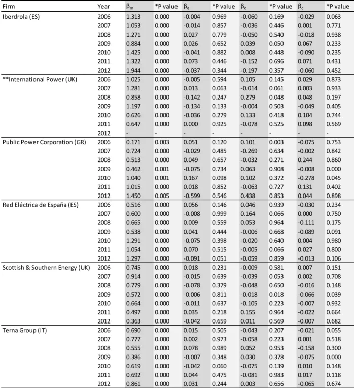
VII. Appendix
Table A
The estimation results of the βm ,βe ,βo ,βc (84 individual regressions)
Firm Year βm *P value βe *P value βo *P value βc *P value
a2a (IT) 2006 0.484 0.000 0.054 0.576 0.037 0.871 0.012 0.248
2007 0.773 0.000 -0.006 0.883 0.012 0.483 0.001 0.141
2008 0.781 0.000 0.014 0.797 0.026 0.732 -0.015 0.223
2009 1.028 0.000 0.060 0.729 0.177 0.011 -0.232 0.023
2010 1.060 0.000 0.004 0.056 -0.039 0.854 -0.052 0.043
2011 0.902 0.000 0.007 0.886 -0.033 0.731 0.191 0.002
2012 1.604 0.000 0.072 0.233 0.317 0.849 -0.094 0.733
Drax Group (UK) 2006 0.589 0.000 -0.029 0.853 0.332 0.013 0.023 0.508
2007 0.684 0.000 -0.039 0.061 0.334 0.002 -0.009 0.000
2008 0.558 0.000 0.009 0.513 0.295 0.112 0.154 0.208
2009 0.682 0.000 0.011 0.630 0.126 0.041 -0.007 0.423
2010 0.793 0.000 0.045 0.730 -0.069 0.744 0.058 0.784
2011 0.541 0.000 0.154 0.277 0.034 0.101 0.024 0.310
2012 0.542 0.000 0.063 0.164 0.024 0.925 0.004 0.195
Électricité de France (FR) 2006 1.089 0.000 0.048 0.044 0.148 0.343 0.000 0.508
2007 0.916 0.000 -0.031 0.479 0.036 0.097 0.000 0.845
2008 1.056 0.000 -0.067 0.097 0.096 0.712 0.201 0.069
2009 1.272 0.000 0.009 0.718 -0.088 0.071 0.003 0.226
2010 1.158 0.000 0.035 0.981 -0.023 0.531 0.122 0.869
2011 1.297 0.000 -0.071 0.912 0.015 0.335 -0.007 0.263
2012 1.349 0.000 -0.064 0.566 0.031 0.559 0.082 0.539
Endesa (ES) 2006 1.275 0.000 -0.028 0.467 -0.071 0.025 -0.008 0.442
2007 0.041 0.007 -0.008 0.100 0.023 0.564 -0.001 0.923
2008 0.891 0.000 -0.049 0.454 -0.159 0.891 0.015 0.573
2009 0.892 0.000 0.070 0.783 0.034 0.047 -0.051 0.124
2010 1.205 0.000 0.052 0.046 -0.045 0.362 0.021 0.865
2011 1.052 0.000 0.006 0.788 0.093 0.004 0.009 0.345
2012 1.374 0.000 0.086 0.883 -0.042 0.802 -0.034 0.732
Enel (IT) 2006 0.640 0.000 0.019 0.907 -0.073 0.038 -0.018 0.970
2007 0.719 0.000 -0.011 0.873 -0.015 0.806 0.000 0.763
2008 0.986 0.000 0.001 0.062 -0.051 0.776 -0.035 0.989
2009 0.983 0.000 0.015 0.709 0.025 0.600 -0.064 0.788
2010 1.032 0.000 0.006 0.707 0.066 0.005 -0.027 0.101
2011 1.341 0.000 0.130 0.009 -0.087 0.191 0.014 0.882
2012 1.528 0.000 0.048 0.460 -0.056 0.867 -0.138 0.100
Fortum (FI) 2006 1.305 0.000 0.026 0.065 0.128 0.766 0.103 0.000
2007 0.870 0.000 0.024 0.265 0.115 0.118 0.002 0.109
2008 0.906 0.000 -0.009 0.620 0.279 0.019 0.157 0.001
2009 0.968 0.000 -0.045 0.763 0.245 0.058 -0.018 0.055
2010 0.606 0.000 0.102 0.789 0.139 0.102 -0.033 0.289
2011 0.639 0.000 0.038 0.925 0.233 0.019 0.093 0.020
25
Table A continued
The estimation results of the βm ,βe ,βo ,βc (84 individual regressions)
Firm Year βm *P value βe *P value βo *P value βc *P value
Iberdrola (ES) 2006 1.313 0.000 -0.004 0.969 -0.060 0.169 -0.029 0.063
2007 1.053 0.000 -0.014 0.857 -0.036 0.446 0.001 0.771
2008 1.271 0.000 0.027 0.779 -0.050 0.540 -0.018 0.938
2009 0.884 0.000 0.026 0.652 0.039 0.050 0.067 0.233
2010 1.425 0.000 -0.041 0.882 0.008 0.448 -0.090 0.235
2011 1.322 0.000 0.073 0.446 -0.152 0.696 0.071 0.431
2012 1.944 0.000 -0.037 0.344 -0.197 0.357 -0.060 0.452
**International Power (UK) 2006 1.025 0.000 -0.005 0.594 0.105 0.145 0.029 0.873
2007 1.281 0.000 0.013 0.063 -0.014 0.061 0.003 0.933
2008 0.858 0.000 -0.142 0.247 0.279 0.048 0.048 0.197
2009 1.197 0.000 -0.134 0.133 -0.004 0.503 -0.049 0.405
2010 0.626 0.000 -0.036 0.279 0.133 0.418 0.104 0.744
2011 0.647 0.000 0.000 0.925 -0.078 0.525 0.098 0.569
2012 - - -
-Public Power Corporation (GR) 2006 0.171 0.003 0.051 0.120 0.101 0.003 -0.075 0.753
2007 0.724 0.000 -0.029 0.485 -0.269 0.634 -0.002 0.842
2008 0.513 0.000 0.049 0.657 -0.032 0.271 0.244 0.860
2009 0.462 0.001 -0.075 0.734 0.063 0.908 -0.008 0.000
2010 1.040 0.001 0.167 0.098 0.102 0.372 -0.278 0.045
2011 1.015 0.000 0.018 0.852 -0.063 0.727 0.131 0.402
2012 1.450 0.005 -0.599 0.546 0.438 0.853 0.044 0.898
Red Eléctrica de España (ES) 2006 0.516 0.000 0.056 0.146 0.046 0.939 -0.030 0.234
2007 0.600 0.000 -0.008 0.999 0.164 0.066 0.000 0.750
2008 0.665 0.000 0.009 0.559 0.053 0.964 -0.111 0.175
2009 0.538 0.000 0.041 0.444 -0.006 0.668 -0.089 0.091
2010 1.291 0.000 -0.075 0.398 -0.020 0.640 0.004 0.980
2011 1.054 0.000 0.070 0.515 -0.005 0.066 0.027 0.800
2012 1.297 0.000 -0.091 0.051 -0.059 0.859 -0.013 0.106
Scottish & Southern Energy (UK) 2006 0.745 0.000 0.018 0.231 -0.009 0.581 0.007 0.151
2007 0.914 0.000 -0.015 0.639 -0.039 0.053 0.002 0.708
2008 0.779 0.000 -0.078 0.379 -0.048 0.650 -0.016 0.148
2009 0.572 0.000 -0.006 0.811 -0.018 0.018 -0.066 0.039
2010 0.664 0.000 -0.011 0.637 -0.105 0.223 -0.007 0.932
2011 0.497 0.000 0.035 0.218 0.155 0.964 -0.022 0.664
2012 0.363 0.000 -0.042 0.659 0.011 0.569 -0.007 0.682
Terna Group (IT) 2006 0.690 0.000 0.015 0.505 -0.043 0.207 -0.021 0.055
2007 0.777 0.000 0.002 0.973 -0.058 0.223 0.001 0.518
2008 0.555 0.000 0.078 0.989 0.052 0.953 -0.158 0.300
2009 0.386 0.000 -0.007 0.348 0.030 0.378 -0.075 0.000
2010 0.619 0.000 -0.042 0.060 -0.075 0.139 0.010 0.148
2011 0.692 0.000 0.044 0.475 -0.081 0.983 0.017 0.118
2012 0.861 0.000 0.031 0.244 0.003 0.656 -0.065 0.674
26
Table B
The estimation results of the βm ,βe ,βo ,βc (30 individual regressions)
Firm EU ETS Phase βm P value βe P value βo P value βc P value
a2a (IT) 1 0.634 0.000 0.006 0.628 -0.002 0.941 0.002 0.115
2 0.785 0.000 0.011 0.651 0.040 0.151 -0.032 0.182
CEZ Group (CZ) 1 0.947 0.000 0.026 0.136 0.117 0.002 0.002 0.358
2 0.642 0.000 0.000 0.997 0.109 0.000 0.094 0.000
Drax Group (UK) 1 0.644 0.000 -0.021 0.227 0.154 0.000 -0.007 0.000
2 0.529 0.000 0.025 0.262 0.073 0.005 0.009 0.675
Électricité de France (FR) 1 0.621 0.000 0.027 0.089 0.061 0.083 0.000 0.967
2 0.880 0.000 -0.053 0.008 0.005 0.816 0.069 0.001
Endesa (ES) 1 0.437 0.000 0.001 0.946 -0.059 0.033 0.001 0.731
2 0.755 0.000 -0.012 0.527 0.035 0.114 -0.021 0.282
Enel (IT) 1 0.565 0.000 0.001 0.861 -0.021 0.246 0.000 0.747
2 0.994 0.000 0.012 0.477 0.009 0.660 -0.016 0.352
E.ON (DE) 1 0.770 0.000 -0.007 0.584 -0.015 0.611 0.001 0.672
2 0.959 0.000 -0.029 0.135 0.038 0.088 0.040 0.037
Fortum (FI) 1 0.492 0.000 0.030 0.044 0.096 0.004 -0.002 0.209
2 0.755 0.000 -0.030 0.129 0.086 0.000 0.104 0.000
Iberdrola (ES) 1 0.858 0.000 -0.005 0.681 -0.042 0.164 0.000 0.905
2 1.198 0.000 -0.021 0.263 -0.041 0.060 0.028 0.143
International Power (UK) 1 1.086 0.000 0.024 0.101 0.070 0.035 0.000 0.909
2 0.761 0.000 -0.058 0.016 0.072 0.007 0.046 0.062
Public Power Corporation (GR) 1 0.742 0.000 0.000 0.993 -0.008 0.863 0.001 0.818
2 0.825 0.000 0.005 0.906 -0.085 0.062 0.056 0.160
Red Eléctrica de España (ES) 1 0.537 0.000 0.005 0.719 0.033 0.275 0.000 0.913
2 0.652 0.000 -0.017 0.343 0.004 0.862 -0.006 0.740
RWE (DE) 1 0.635 0.000 0.018 0.169 -0.005 0.860 0.001 0.531
2 0.856 0.000 -0.025 0.173 0.036 0.089 0.019 0.293
Scottish & Southern Energy (UK) 1 0.672 0.000 0.007 0.547 0.050 0.046 0.000 0.823
2 0.572 0.000 -0.015 0.336 -0.022 0.221 -0.021 0.186
Terna Group (IT) 1 0.422 0.000 0.004 0.690 0.007 0.770 0.000 0.724
2 0.462 0.000 -0.013 0.417 -0.010 0.571 -0.037 0.020
Table C Definitions
Ri The individual European electricity firm's return: ln(pricet/pricet-1)
Rm The market return: ln(pricet/pricet-1)
Re The change in electricity prices: ln(pricet/pricet-1)
Ro The change in oil prices: ln(pricet/pricet-1)
Rc The change in EUA prices: ln(pricet/pricet-1)
*s ource of ea ch da ta s eri es pres ented i n Secti on IV
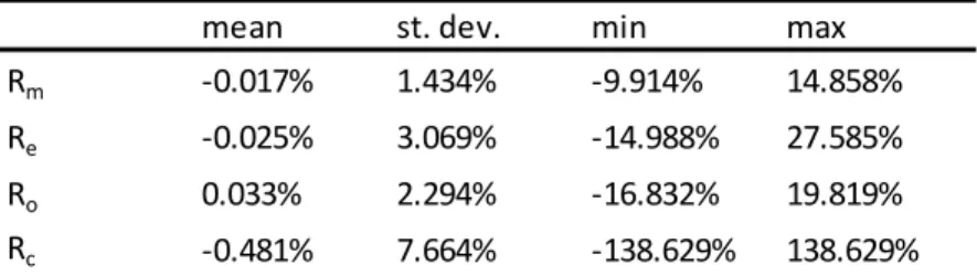
Table D
Descriptive Statistics
mean st. dev. min max
Rm -0.017% 1.434% -9.914% 14.858%
Re -0.025% 3.069% -14.988% 27.585%
Ro 0.033% 2.294% -16.832% 19.819%
27
References
Asselt HV, Biermann F. “European emissions trading and the international competitiveness of energy-intensive industries: a legal and political evaluation of possible supporting measures.” Energy Policy (2007) 497–506.
Bushnell, James B., Howard Chong, and Erin T. Mansur. “Profiting from Regulation:
Evidence from the European Carbon Market.” NBER Working Paper No. 15572 (2012).
Convery, Frank J, and Luke Redmond. “Market Price Developments in the European Union Emissions Trading Scheme.” Review of Environmental Economics and Policy 1 (2007) 88-111.
Ellerman, A. Denny, and Barbara K. Buchner. “The European Union Emissions Trading Scheme: Origins, Allocation, and Early Results.” Review of Environmental Economics and Policy 1 (2007) 66-87.
Ellerman AD, Buchner B. “Over-allocation or abatement? A preliminary analysis of the EU emissions trading scheme based on the 2005 emissions data.” Working paper (2006).
European Commission Climate Action. “The EU Emission Trading Scheme.”
http://ec.europa.eu/clima/policies/ets/. (2007).
European Commission Climate Action. “Structural reform of the European carbon market.”
http://ec.europa.eu/clima/policies/ets/reform/index_en.htm (2013).
Hoffmann VH. “EU ETS and investment decisions: the case of the German electricity industry.” European Management Journal (2007) 464–74.
Kruger, Joseph, Wallace E. Oates, and William A. Pizer. “Decentralization in the EU
28
Mo, Jian-Lei, Lei Zhu, and Ying Fan. “The impact of the EU ETS on the corporate value o European electricity corporations.” Energy 45 (2012) 3-11.
Oberndorfer, Ulrich. “EU Emission Allowances and the stock market: Evidence from the electricity industry.” Ecological Economics 68 (2009) 1116-1126.
Sercu, Piet, Martina Vandebroek, and Tom Vinaimont. “Thin-trading Effects in Beta: Bias v. Estimation Error.” Working Paper (2007).