2018_Larsen.pdf

(1)

Selecting Generative Models for Networks using Classification with

Machine Learning

Nicholas Alfredo Larsen

An undergraduate senior honors thesis submitted to the faculty of the University of North Carolina at Chapel Hill in fulfillment of the requirements for the Honors Carolina Senior Thesis in the Department of Statistics and Operations Research.

Chapel Hill 2018

To be approved by:

Peter J. Mucha

Nicolas Fraiman

(2)

(3)

ABSTRACT

NICHOLAS A. LARSEN: Model Selection with Machine Learning for Classifying Network Community Structures

(Under the direction of Peter J. Mucha, Shankar Bhamidi, and Nicolas Fraiman)

(4)

To my mentors, Peter Mucha and Natalie Stanley, who became my academic family.

(5)

ACKNOWLEDGEMENTS

It goes without saying that I would acknowledge my primary advisor, Peter Mucha, for his advice and direction in implementing this project. What is, perhaps, less obvious is my sincere gratitude for having a role-model who goes above and beyond his role as an academic advisor. To this day I am not sure why he took on a freshman undergraduate with no coding experience, but I will always be grateful he did. I am truly honored to have benefited from Peter’s mentorship; our subsequent weekly meetings have been an invaluable experience and have included some of the most stimulating conversations during my time at Carolina. I have learned so much beyond network science - from the realities of administration and research in the “real world” to what pro time management looks like - that listing them under the Acknowledgements section in an undergraduate thesis would be a bit

ridiculous. Thank you for always making me feel welcome.

Behind any undergraduate researcher, there is a graduate student who actually knows what the project is about. I would like to thank Natalie Stanley not only for her friendship, but also for showing me what true persistence and initiative looks like. Yours is the standard that I have set for myself as I enter graduate school.

Many thanks to the Mucha research group, whose meetings have served as a collective role-model and became a weekly highlight. I would also like to thank Shankar Bhamidi, who despite an extraordinarily busy year sponsored an extra undergraduate student and put so much effort into writing recommendation letters and providing useful insights in my search for graduate schools. Thank you also to Nicolas Fraiman, who got on board with such short notice.

(6)

LIST OF TABLES

2.1 Summary of Total Number of SBMs and Instance Graphs. For each SBM, we generated 100 instance graphs for use in evaluating the

discrimi-natory power over these sets of SBM parameters. . . 9

2.2 Summary of SBM parameters used for classification of graphs of same type, where only the number of communities differ. Networks generated by these models were used in sections 2.3.2 and 2.5.1.nis the number of nodes for each graph, pij represents the(i, j)th entry in the probability matrices. In the case of the core-periphery structure,λis the rate of exponential decay as defined earlier. The parameters summarized here represent total of 15 SBMs with three models per graph type, one for

eachk. . . 9

2.3 Summary of SBM parameters used for classification of graphs of the same type, where each label corresponds to a probability matrix with different parameter values. See tables 2.4, 2.5, and 2.6 for summary of the core-periphery structure parameters. Networks generated by these models were used in sections 2.3.3 and 2.5.2. For all graph types we have fixed the number of communities at 5. In the case of the random graphs, values ofphave been chosen to generate graphs with a range of densities. Smaller values ofpindicate low edge probability, resulting in sparser networks. Conversely, aspincreases, the network density grows as well. For assortative graphs, we have fixed inter-community probability as 0.5and vary the between-community edge probabilities (pij wherej 6=i). Aspij increases, the assortative structure more closely resembles that of a random graph. The disassortative parameters mimic the assortative case, in that we only varypij. Values ofpij are selected such that nodes in graphs from differing labels are twice as likely or half as likely to connect to nodes in other communities. Other parameters for the disassortative graphs are selected as dense and sparse counterparts. The parameters for the ordered graphs are selected such that two labels have the same value

forpii−pi,i±1and other labels are slightly sparser or denser versions. . . 10

2.4 Parameter Summary for Core-periphery Case, Sub-Experiment 1. (Referenceitem 5 in section 2.1 for notation.) Networks generated by these models were used in sections 2.3.3 and 2.5.2. Labels 0, 1, and 2 correspond to networks with strong inner-core edge probability (P0) with

varying rates of decay (λ). Labels 3, 4, and 5 test the same idea with a weaker inner-core edge probability. Labels 6 and 7 were used to test classification problems where networks have the same inner-core edge probabilities and similar rates of decay. They were tested with labels 0 and

3 respectively. . . 10

(9)

2.5 Parameter Summary for Core-periphery Case, Sub-Experiment 2. Labels 8 and 9 were used for testing discriminatory power in the case of similar cores and decay rates when the networks are dense. Labels 10 and 3 were used for the same purpose except for sparse networks.

Networks generated by these models were used in sections 2.3.3 and 2.5.2. . . 10

2.6 Parameter Summary for Core-periphery Case, Sub-Experiment 3. Labels 0, 3, and 11 were used for discriminating graphs with the same decay rateλ= −0.5but very different inner-core probabilities. Labels 0, 12, and 13 were used as a case for sameλand similar large inner-core probabilities, and labels 3, 14, and 15 provided an analogous case for similar small inner-core probabilities. Labels 5 and 16 were used for test-ing classification when inner-core probabilities are small and similar with identical high rates of decay. Labels 8 and 18 test the same idea for large inner-core probabilities and a lower rate of decay. Networks generated by

these models were used in sections 2.3.3 and 2.5.2. . . 11

2.7 RF Accuracy Scores for Discriminating between Graphs ofk={3,5,8}

on a Flattened Adjacency Matrix Feature Space. Random and Core-periphery graphs are shown to be the easiest to classify when using random forests with flattened adjacency matrices. Keeping in mind that classifying by random chance is equivalent to rolling a three-sided die (1₃ probabil-ity), the accuracy scores in this table suggest that random forests can discriminate between graphs of the same type with different numbers of

communities fairly well and better than random chance in all cases. . . 12

2.8 Random Forest Classification Accuracy on Random and Assortative Graphs Sets. See table 2.3 for the parameters corresponding to each label. The first row tests random forests’ discriminatory power on a wide range of graph parameters. The second and third rows test binary classification

scenarios when graphs have approximately similar density. . . 13

2.9 Random Forest Classification Accuracy on Disassortative and Ordered Graphs Set.See table 2.3 for the parameters corresponding to each label. The first row tests random forests’ discriminatory power on a wide range of graph parameters. For the disassortative graphs, labels 0, 1, and 2 represent probability matrices that have the same diagonal values, but with off-diagonal values that differ by factors of 2. For the ordered graphs, these labels represent probability matrices where the differences between on- and off-diagonal values is approximately 0.2. The last two rows test binary classification scenarios when graphs have approximately similar

density. . . 13

2.10 RF Classification Accuracy Summary for Core-periphery Case, Sub-Experiment 1. See table 2.4 for a summary of the parameters. The first two rows correspond to classification accuracy when the parametersλare fairly different. The last two rows correspond to classification scenarios

(10)

2.11 RF Classification Accuracy Summary for Core-periphery Case,

Sub-Experiment 2. See table 2.5 for a summary of the parameters. . . 15 2.12 RF Classification Accuracy Summary for Core-periphery Case,

Sub-Experiment 3.See table 2.6 for a summary of the parameters. . . 15 2.13 RF Accuracy Scores from Discriminating between Graphs of k =

{3,5,8}on a Network Statistics Feature Space.Accuracy scores from classifying on a held-out test set, using the same data and classification set

up as described in table 2.7. . . 20

2.14 RF RF classification scores between graphs of differing M matri-ces on a network statistics feature space for random and assortative graphs. Accuracy scores from classifying on a held-out test set, using the

same data and classification set up as described in table 2.8. . . 20

2.15 RF classification scores between graphs of differingM matrices on a network statistics feature space for ordered and disassortative graphs.

*For ordered graphs, the label set L0, L1, L2 represents graphs whose M matrices have similar differences Mii−Mi,i±1. In the case of the

disassortative graphs, the set L0, L1, L2 corresponds toM matrices with

the same on-diagonal values. . . 21

2.16 RF classification scores for core-periphery graphs, sub-experiment 1, on a network statistics feature space.Reference table 2.4 for a summary of relevant SBM parameters and section 2.3.3 for a description of the

experimental set-up. . . 21

3.1 Average Densities of 4- and 5-Block MixNet Realizations.As reflected in this table, the models fitted to the macaque data set produce graphs of roughly the same density. In this case, the average densities over all realizations used for this experiment are shown. Intuitively, one may expect any classifier to perform poorly once graphs achieve a certain level of similarity with respect to their densities, particularly if one notices that many of our features in section 2.4.1 are closely related to graph density. However, as shown in Caceres et al. (2016) and later in this section, random forests discriminatory power remains quite strong as long as the underlying

edge-probabilities remain relatively distinct. . . 30

(11)

LIST OF FIGURES

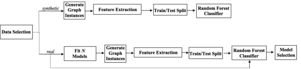
1.1 Methodology Pipeline. A schematic of the methods implemented in this research. The top branch is a framework for experiments on synthetic data sets. The lower branch outlines the steps for using random forests to select the best generative model for real data. The arrow connecting “real” to “Random Forest Classifier” means once the classifier is trained on instances from theM models, we input the original data set into the classifier. The classifier will then match the original data to the model it

deems most similar. . . 4

2.1 Table 1 inCaceres et al. (2016). This figure presents the parameters used for testing the random forests’ ability to discriminate between Erd˝os-R´enyi

models and assortative SBMs. . . 9

2.2 Summary of Classification Accuracies when Varying Number of

Com-munities.Results from tables 2.7 and 2.13. . . 23 2.3 Summary of Classification Accuracies when Varying SBM

Probabil-ity Matrices. Results from tables 2.8, 2.9, 2.14, & 2.15. The lefthand column summarizes random forest classification accuracies on the flat-tened adjacency matrix feature space for experiments using all graph types, excluding core-periphery graphs. The righthand column does the same for

the network statistics feature space. . . 24

2.4 Summary of Classification Accuracies when Varying SBM Probabil-ity Matrices (core-periphery graphs). Results from tables providing accuracy scores from both feature spaces for the sub-experiments using core-periphery graph types. Red columns correspond to results from classi-fiers trained on the flattened adjacency matrix feature space, blue columns

correspond to those trained on the network statistics feature space. . . 25

3.1 Summary of Mixer Models fitted to the Macaque data set. Top left: ICL vs number of communities per model. The dotted red line indicates that the 4-community MixNet model maximizes ICL and is therefore the best fit to the macaque data set. This model serves as thegold standard with which to compare the our own “best model” chosen by random forests. Top right: Adjacency matrix organized under the best model. Bottom left: Degree distribution.Bottom right: Schematic of probability

strength between and within communities under the best model. . . 27

3.2 Adjacency Matrices of Original Macaque Data with 4- and 5-Block Realizations.Using the methods described in section 3.1, SBMs of 4 and 5 blocks were estimated for the macaque data set. The original adjacency matrix (left) and two realizations of the 4- and 5-block models (top and

(12)

3.3 Random Forests as a Model Selection Criterion. Left: Classification accuracy versus number of trees for random forests modeled on flattened adjacency matrices of the instance graphs and original data set. Right: Classification accuracy versus number of trees for random forests modeled on network statistics (section 2.4.1) of the instance graphs and original data set. For both plots smoothed lines of fit are given, with grey areas

representing standard error. . . 33

(13)

LIST OF ABBREVIATIONS

SBM Stochastic Block Model

ICL Integrated Completed Likelihood

RF Random Forests

(14)

CHAPTER 1

Introduction

(15)

a feature space, and 3) using the built-in feature ranking aspect of random forests to potentially alleviate the “black box” problem that can occur when trying to understand why a particular model has been chosen as a best fit to the data.

We conclude Chapter 1 with a brief overview of some of the literature in network model selection and classification, with more in-depth descriptions provided later as needed, as well as a statement about our motivation and goals. In Chapter 2, we introduce a type of generative model for networks called the Stochastic Block Model (SBM) and describe the discriminatory power of random forests when classifying instances of these models. In Chapter 3, we describe a subtype of the SBM and fit several to a brain connectivity networks data set, using random forests as a model selection criteria and comparing it to an established metric for model selection called Integrated Completed Likelihood (ICL). Our conclusions and future directions are presented in Chapter 4.

1.1 Overview of Network Classification and Modeling

(16)

results, in that random forests can very accurately label instances of SBMs with the correct model for certain graph types, presuming the model parameters are sufficiently different from one another (Caceres et al., 2016).

The sheer number of possible underlying structures that occur in networks has lead to a variety of techniques designed to develop generative models aimed at capturing these properties. Some methods focus on taking advantage of any community structure inherent in the network to devise a metric for community detection (Fortunato, 2010; Newman, 2006; Girvan and Newman, 2002), while others use empirical data to estimate the parameters governing a network’s underlying large scale structure (Daudin et al., 2008; Holland et al., 1983; Airoldi et al., 2008). A particularly intriguing model selection criterion is the one proposed by Peixoto (2015). Peixoto notes the difficulties that arise when attempting to compare models that result in diverging descriptions of the same network. To compensate, Peixoto proposes a model selection procedure based on the minimum description length principle. As in this thesis, Peixoto also tests this principle using the stochastic block model and its variants, as well as on a number of empirical network data sets, illustrating the efficiency and scalability of his algorithm. In this thesis, we chose to use the generative model structure proposed by Daudin et al. (2008) and used the model selected by the modified selection criteria defined by Daudin et al. (2008) and originally established by Biernacki et al. (2000) as our gold standard with which to compare random forests’ performance. Further information describing Daudin et al. (2008)’s work is presented in section 3.1.2.

1.2 Motivation and Goals

The motivation for this research was inspired by the following question: given a set ofN generative models fit to a networks data set, can a random forests classifier trained on a fixed number of instances from each model choose the best model when asked to classify the original data set? Research conducted by Cacereset al.inA Model Selection Framework for Graph-based Dataasked a similar question in a narrower context, exploring the discriminatory power of random forests within the parameter space of the Erd˝os-R´enyi and simple stochastic block models (SBM) and using a framework similar to figure 1.1. While thorough in exploring the behavior of random forests with respect to these two simple models, this research did not account for the variety of SBM types that

(17)

Figure 1.1:Methodology Pipeline.A schematic of the methods implemented in this research. The top branch is a framework for experiments on synthetic data sets. The lower branch outlines the steps for using random forests to select the best generative model for real data. The arrow connecting “real” to “Random Forest Classifier” means once the classifier is trained on instances from theM models, we input the original data set into the classifier. The classifier will then match the original data to the model it deems most similar.

can occur, nor did it explore how to use random forests for choosing the best generative model for a real data set. This honors thesis aims to incorporate these additional facets that, to the knowledge of the authors, have not been examined in the previous research.

(18)

CHAPTER 2

Experiments with Synthetic data sets

To the current knowledge of the authors, the extent of literature exploring the behavior of random forests in the context of network classification and model selection amounts only to the work conducted by Caceres et al. (2016), whose findings are discussed in section 2.2. The key differences between our results and those presented by Caceres et al. (2016) are 1) we explore a much more substantial range of graph types and parameters and 2) we use random forests as a model selection criterion and compare this to other accepted model selection methods (see Chapter 3). Other related research conducted by Canning et al. (2017) and Barnett et al. (2016) that uses random forests for network classification focused more on comparing random forests to other machine learning techniques or simply determining the discriminatory power of network classification by random forests on synthetic or applied data sets, rather than exploring the general behavior of random forest classification in the context of networks.

(19)

(section 2.5). The feature sets were split multiple times into training and test sets used to build and test classification accuracy of a random forest model. For each split, the models were trained over a parameter space ofntrees ={100,200,300,400,500}using 10-fold cross-validation to select the best model for calculating prediction accuracy.

2.1 Introduction to Stochastic Block Models

Aaron Clauset’sNetwork Analysis and Modelingonline lecture notes provided the main template for determining which type of SBM structures to employ in these analyses (Clauset, 2013). Using Clauset’s notation, the general stochastic block model is comprised of ak×kprobability matrix M where the entryi, jgives the probability of a vertex in communityiconnecting to a vertex in communityjandkrepresents the number of communities in the model. SBMs typically also include ann×1scalar vector that stores the community membership of a node, wherenis the number of nodes in the graph. To generate a graph instance of an SBM, simply loop through eachi, j’th pairing and generate an edge with probabilityMij. In other words, the probability for each element in a graph adjacency matrixAgenerated from an SBM with probability matrixM is defined as,

P(Aij = 1)∼Bernoulli(Mij) (2.1)

Clauset’s lecture identifies five basic SBM structures which are used as the basis for these experiments, referred to in this paper asgraph typesortype(Clauset, 2013).

1. Random Graphs: Another name for the Erd˝os-R´enyi graph model, where edge-probabilities are the same for all nodes in all communities.

Mij =pconstant∀i, j∈ {1, ..., k} (2.2)

(20)

Mii> Mij fori6=j (2.3)

3. Disassortative Graphs: The opposite of assortative graphs, these produce a structure where a given node is more likely connect to nodes outside of its community than within. These matrices have strong off-diagonal components and weak on-diagonals.

Mii< Mij fori6=j (2.4)

4. Ordered Graphs: These are similar to assortative graphs in that vertices of the same community are more likely to be connected, with the additional characteristic of being closely connected to adjacent communities. In terms of matrix structure, these SBMs resemble assortative graphs with strong first-off-diagonal components.

Mii≈Mi,i−1 ≈Mi,i+1 (2.5)

5. Core-periphery Graphs: The core-periphery structure is a subtype of ordered graph, where the probability of an edge decreases exponentially with community index. It may be helpful to think of the probability matrix as containing one large “core” probability which serves as the initial quantity in a system subject to an exponential decay by which the subsequent probabilities are defined. This creates anested core structurewhere community densities decrease with community index. In general terms,M is defined as

Mk×k =



 

 

P0e−λ(j−1) whenjis on the diagonal

P0e−λ(j) whenjis off the diagonal

whereP0=M1,1,λis the rate of probability decay, andj= 1, ..., kis a column index. Here

we also briefly provide a rough intuition behind the effect of core-periphery parametersλ andP0. As| λ |→ ∞, the edges located in the outer-cores of the graph begin to drop of

exponentially, resulting in single nodes surrounding a small core of nodes connected with probabilityP0. As|λ|→0, subsequent probabilitiesMij approachP0, making the network

(21)

more closely resemble a random structure. Large values ofP0typically mean larger values in

Mij, which translates into more densely connected graphs. In generating dozens of different SBMs with the core-periphery structure, we also observed, at least from a visual point of view, that the effect ofλon the number of edges in the graph appears to be much stronger than that ofP0.

2.2 Motivation for Synthetic Experiments and Description of SBM

Pa-rameters

(22)

Figure 2.1:Table 1 inCaceres et al. (2016). This figure presents the parameters used for testing the random forests’ ability to discriminate between Erd˝os-R´enyi models and assortative SBMs.

Total SBMs Total Graphs

58 5800

Table 2.1: Summary of Total Number of SBMs and Instance Graphs. For each SBM, we generated 100 instance graphs for use in evaluating the discriminatory power over these sets of SBM parameters.

decided to break up the set of core-periphery graphs of varying probability matrices into three general categories. The parameter summaries for each category are presented in tables 2.4, 2.5 and 2.6.

2.3 Experiments Using Flattened Adjacency Matrices as a Feature

Space.

2.3.1 Using flattened adjacency matrices as feature sets

For these experiments, random forest models were trained using graph edge-weights, specifically the graphs’ flattened adjacency matrices, as the feature set. In other words, suppose synthetic graphGiis generated from an SBM labeledLj, whereGiis undirected and unweighted with adjacency matrix

Graph Type Parameters(fixed for eachk= 3,5,8) Random n= 50,p= 1/k

Assortative n= 50,pii= 0.5,pij = 0.01j6=i Disassortative n= 50,pii= 0.01,pij = 0.12j6=i Ordered n= 50,pii= 0.5,pi,j±1= 0.3

Core-periphery n= 50, P0,0 = 0.7, λ=−0.50

Table 2.2: Summary of SBM parameters used for classification of graphs of same type, where only the number of communities differ.Networks generated by these models were used in sections 2.3.2 and 2.5.1. nis the number of nodes for each graph,pij represents the(i, j)th entry in the probability matrices. In the case of the core-periphery structure,λis the rate of exponential decay as defined earlier. The parameters summarized here represent total of 15 SBMs with three models per graph type, one for eachk.

(23)

Graph Type Label 0 Label 1 Label 2 Label 3 Label 4

Random (n= 50,k= 5) p= 0.035 p= 0.05 p= 0.1 p= 0.2 p= 0.5

Assortative (n= 100,k= 5,pi,i= 0.5) pi,j= 0.01 pi,j= 0.02 pi,j= 0.05 pi,j= 0.10 pi,j= 0.25

Disassortative (n= 50,k= 5,pi,i= 0.5) pi,i= 0.01 pi,i= 0.01 pi,i= 0.01 pi,i= 0.011 pi,i= 0.012

pi,j= 0.12 pi,j= 0.24 pi,j= 0.06 pi,j= 0.058 pi,j= 0.28

Ordered (n= 75,k= 5) pi,i= 0.5 pi,i= 0.3 pi,i= 0.7 pi,i= 0.31 pi,i= 0.68

pi,j±1= 0.2 pi,j±1= 0.1 pi,j±1= 0.5 pi,j±1= 0.085 pi,j±1= 0.55

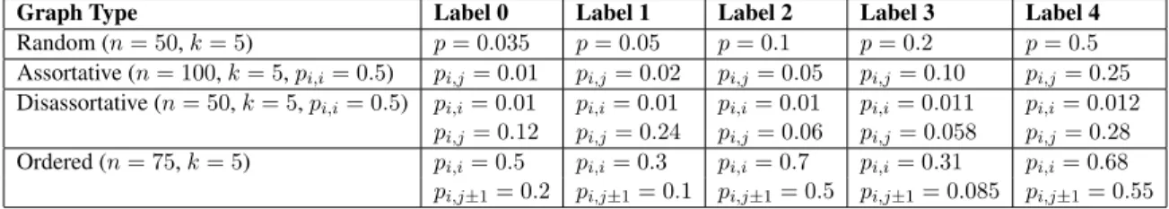
Table 2.3: Summary of SBM parameters used for classification of graphs of the same type, where each label corresponds to a probability matrix with different parameter values. See tables 2.4, 2.5, and 2.6 for summary of the core-periphery structure parameters. Networks generated by these models were used in sections 2.3.3 and 2.5.2. For all graph types we have fixed the number of communities at 5. In the case of the random graphs, values ofphave been chosen to generate graphs with a range of densities. Smaller values ofpindicate low edge probability, resulting in sparser networks. Conversely, aspincreases, the network density grows as well. For assortative graphs, we have fixed inter-community probability as0.5and vary the between-community edge probabilities (pij wherej6=i). Aspij increases, the assortative structure more closely resembles that of a random graph. The disassortative parameters mimic the assortative case, in that we only varypij. Values ofpij are selected such that nodes in graphs from differing labels are twice as likely or half as likely to connect to nodes in other communities. Other parameters for the disassortative graphs are selected as dense and sparse counterparts. The parameters for the ordered graphs are selected such that two labels have the same value forpii−pi,i±1and other labels are slightly sparser

or denser versions.

Label P0 λ

Label 0 0.7 -0.5 Label 1 0.7 -0.2 Label 2 0.7 -0.7 Label 3 0.55 -0.5 Label 4 0.55 -0.2 Label 5 0.55 -0.7 Label 6 0.7 -0.45 Label 7 0.55 -0.45

Table 2.4: Parameter Summary for Core-periphery Case, Sub-Experiment 1. (Referenceitem 5in section 2.1 for notation.) Networks generated by these models were used in sections 2.3.3 and 2.5.2. Labels 0, 1, and 2 correspond to networks with strong inner-core edge probability (P0)

with varying rates of decay (λ). Labels 3, 4, and 5 test the same idea with a weaker inner-core edge probability. Labels 6 and 7 were used to test classification problems where networks have the same inner-core edge probabilities and similar rates of decay. They were tested with labels 0 and 3 respectively.

Label P0 λ

Label 8 0.7 -0.3 Label 9 0.72 -0.32 Label 10 0.58 -0.52

(24)

Label P0 λ

Label 11 0.85 -0.5 Label 12 0.74 -0.5 Label 13 0.78 -0.5 Label 14 0.59 -0.5 Label 15 0.63 -0.5 Label 16 0.57 -0.7 Label 17 0.73 -0.3

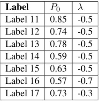
Table 2.6: Parameter Summary for Core-periphery Case, Sub-Experiment 3. Labels 0, 3, and 11 were used for discriminating graphs with the same decay rateλ=−0.5but very different inner-core probabilities. Labels 0, 12, and 13 were used as a case for sameλand similar large inner-core probabilities, and labels 3, 14, and 15 provided an analogous case for similar small inner-core probabilities. Labels 5 and 16 were used for testing classification when inner-core probabilities are small and similar with identical high rates of decay. Labels 8 and 18 test the same idea for large inner-core probabilities and a lower rate of decay. Networks generated by these models were used in sections 2.3.3 and 2.5.2.

Ai ∈Rn×n. The corresponding feature vector forGi, the so-called “flattened adjacency matrix”, is a row vector of zero’s and one’s.

vec(Ai)T =Fi ∈R1×(n×n) (2.6)

2.3.2 Classification of graphs of same type, where only the number of communities differ.

For each graph type in section 2.1, three sets of SBMs were defined. The only parameter that varied was the number of communities,k, wherek= 3,5,8. Table 2.2 is a summary of the graph types and corresponding parameters that were fixed askvaried.

For each SBM, 100 instance graphs were generated and their flattened adjacency matricesFi extracted. An instance graph was labeled by the number of communities of the corresponding parent SBM. Random forest classifiers were trained on 67%of the data and accuracy scores from classifying the held-out 33%were used to estimate the models’ test accuracies. Generally speaking, random forests seem able to discriminate fairly accurately between SBM instances of the same type with differing numbers of communities. Visually speaking, the structural differences between these graph classes were easy to spot. In many cases, strong classification accuracies seemed to follow the cases where graph instances of different communities exhibited very different structures. The

(25)

Graph Type Accuracy Score

Random 87.85±10.66 Assortative 61.89±16.11 Disassortative 38.11±19.36 Ordered 81.0±15.86 Core-periphery 83.89±12.76

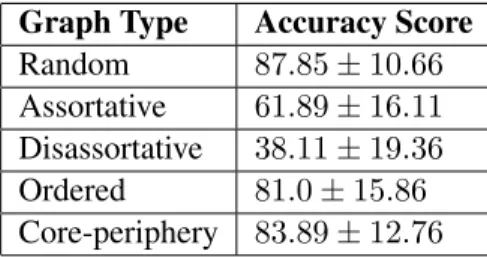
Table 2.7: RF Accuracy Scores for Discriminating between Graphs ofk ={3,5,8}on a Flat-tened Adjacency Matrix Feature Space.Random and Core-periphery graphs are shown to be the easiest to classify when using random forests with flattened adjacency matrices. Keeping in mind that classifying by random chance is equivalent to rolling a three-sided die (1₃ probability), the accuracy scores in this table suggest that random forests can discriminate between graphs of the same type with different numbers of communities fairly well and better than random chance in all cases.

one exception, seen in the low accuracy score of the disassortative experiment, corresponded to a case where it was very difficult to visually distinguish the graph types. A likely contributing factor to the lower classification score is that the parameter values of the corresponding SBMs of these graphs varied perhaps the least out all the experiments. Both the results in Caceres et al. (2016) and subsequent experiments in section 2.5 also suggest that the discriminatory power of random forests decreases as SBM parameters become more similar.

2.3.3 Classify graphs of the same type, where each label corresponds to a probability matrix with different parameter values.

The possibilities for combinations of different SBM parameters within a graph type resulted in a slightly more involved series of experiments than those described above. For each graph type, a set of SBMs were defined in such a way to give a wide range of graph parameters. As in section 2.3.2, 100 instance graphs were generated for each of the SBMs used in an experiment and random forest classifiers were trained on 67% of the data and tested on the remaining 33%. Graphs were assigned a unique label corresponding to their parent SBM. The following discussion summarizes each experiment (corresponding to graph type).

(26)

Label Set Random Assortative

L0, L1, L2, L3, L4 60.22±11.07 43.00±09.71 L0, L1 (sparse case) 67.46±18.97 49.37±15.78 L2, L3 (dense case) 95.08±8.71 90.87±10.52

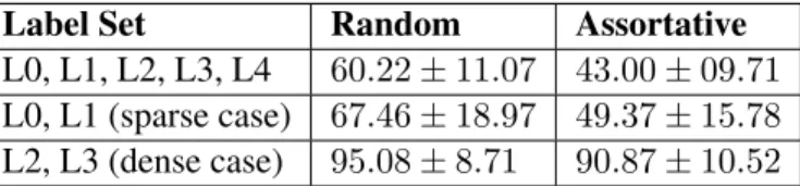
Table 2.8: Random Forest Classification Accuracy on Random and Assortative Graphs Sets. See table 2.3 for the parameters corresponding to each label. The first row tests random forests’ discriminatory power on a wide range of graph parameters. The second and third rows test binary classification scenarios when graphs have approximately similar density.

Label Set Disassortative Ordered

L0, L1, L2, L3, L4 46.56±11.22 48.60±11.24 L0, L1, L2 66.70±16.13 91.96±8.73 L2, L3 (sparse case) 52.30±18.13 53.57±22.06 L1, L4 (dense case) 53.73±21.58 55.40±22.07

Table 2.9:Random Forest Classification Accuracy on Disassortative and Ordered Graphs Set.

See table 2.3 for the parameters corresponding to each label. The first row tests random forests’ discriminatory power on a wide range of graph parameters. For the disassortative graphs, labels 0, 1, and 2 represent probability matrices that have the same diagonal values, but with off-diagonal values that differ by factors of 2. For the ordered graphs, these labels represent probability matrices where the differences between on- and off-diagonal values is approximately 0.2. The last two rows test binary classification scenarios when graphs have approximately similar density.

accuracy also increases. Differences between the parameters for L0 and L1 were not as large as differences between parameters for L2 and L3 due to the relatively smaller probability values for the sparser case. As a result, we see the strongest classification scores in the final row of table 2.8. A similar case can be made for table 2.9, except notice that the largest differences in parameters occurred for the L0, L1, L2 label set, rather than the sparse and dense label sets.

In general, the results in tables 2.8 and 2.9 tell us that when parameters of SBMs are selected to produce instance graphs of similar parameters, even if graph density is similar, random forests’ classification accuracy decreases. However, for sufficient differences in the parameters, even using a feature set as trivial as flattened adjacency matrices allows for strong classification accuracy. For example, consider the classification accuracies for the ordered graph types in table 2.9. When tasked to classify sets of graphs with similar parameters (L2 & L3 and L1 & L4), the random forest models performed barely better than a coin toss. However, when classifying a set of graphs with a wide enough range of parameters (label set L0, L1, L2), classification accuracy jumped to nearly 92 percent.

(27)

Label Set Accuracy

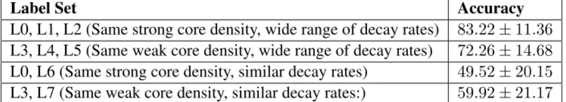
L0, L1, L2 (Same strong core density, wide range of decay rates) 83.22±11.36 L3, L4, L5 (Same weak core density, wide range of decay rates) 72.26±14.68 L0, L6 (Same strong core density, similar decay rates) 49.52±20.15 L3, L7 (Same weak core density, similar decay rates:) 59.92±21.17

Table 2.10: RF Classification Accuracy Summary for Core-periphery Case, Sub-Experiment 1. See table 2.4 for a summary of the parameters. The first two rows correspond to classification accuracy when the parametersλare fairly different. The last two rows correspond to classification scenarios with more similarλ.

Experiments with Core-Periphery graphs: The set of SBMs for the core-periphery graph case is particularly extensive due to the wide range of parameter combination possibilities available. Recall that this particular core-periphery structure is defined by exponentially decreasing probabilities indexed by community. As magnitude of the rate of decay approaches infinity, all that is left is the “core” community with edge-probabilities of nodes in the outer-cores approaching zero and overall density decreasing. As the rate of decay magnitude moves in the opposite direction, approaching zero, overall graph density increases and the core-periphery structure acts more like a random graph, with outer-core edge-probabilities staying very close to the inner-coreP0. In other words, an increased

rate of decay results in a decrease in graph density and a decrease in decay rates results in an increase of graph density. Conversely, largerP0 values give denser graphs, whereas smallerP0 results in

weaker out-core probabilities. In order to take into account the various interactions at play, we devised the three following sub-experiments.

Core-periphery case, sub-experiment 1: Here we defined 8 SBMs designed to provide clas-sification scenarios where random forests discriminated between core-periphery graphs with the sameP0 and differing rates of decay. From the last two rows of table 2.10, one can observe how

the discriminatory power of random forests decreases when it is tasked with classifying graphs of similarλrates. Otherwise, classification accuracy was fairly strong for a wider range of parameter differences.

Core-periphery case, sub-experiment 2: Here we compared 2 sets of graphs defined by similar P0 andλvalues. As expected, classification accuracies were quite low, with both worse than a

random coin toss (table 2.11).

(28)

Label Set Accuracy

L8, L9 (dense case) 46.51±22.48 L3, L10 (sparse case) 47.06±20.02

Table 2.11: RF Classification Accuracy Summary for Core-periphery Case, Sub-Experiment 2. See table 2.5 for a summary of the parameters.

Label Set Accuracy

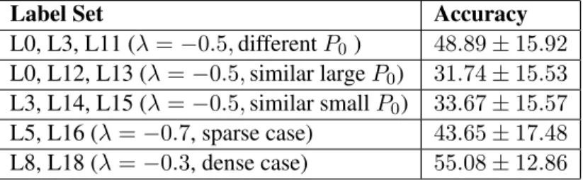
L0, L3, L11 (λ=−0.5,differentP0) 48.89±15.92

L0, L12, L13 (λ=−0.5,similar largeP0) 31.74±15.53

L3, L14, L15 (λ=−0.5,similar smallP0) 33.67±15.57

L5, L16 (λ=−0.7, sparse case) 43.65±17.48 L8, L18 (λ=−0.3, dense case) 55.08±12.86

Table 2.12: RF Classification Accuracy Summary for Core-periphery Case, Sub-Experiment 3.See table 2.6 for a summary of the parameters.

much lower for these scenarios, most likely due to the fact that the rate of decay has a stronger influence on the graph structure thanP0, thus graphs are more similar to one another when their

respectiveλ’s are also similar, regardless of theirP0values.

2.3.4 Summary of results on the flattened adjacency feature space

Generally speaking, when classifying graph instances from models of sufficiently different parameters, random forests were often fairly adept at distinguishing graphs from most SBM types. Clearly, however, accuracy scores varied depending on which graph type was the focus of the experiment. For example, classification scores for ordered graphs in both general experiments varying number of communities and varying probability matrix values were usually quite strong, whereas disassortative graphs seemed to produce lesser accuracy scores in all cases. The relationship between the parameter differences and random forest classification accuracy was also noted by Caceres et al. (2016) for Erd˝os-R´enyi models (random graphs) and the assortative SBM structure.

2.4 Using Network Statistics

In section 2.3, we employed perhaps the most trivial method for converting graphs into a numeric feature space for classification by mapping each graphGi to vector Fi, where Fi = vec(Ai)T. In other words, section 2.3 explored graph classification using one-dimensional vectors of binary variables, where each variable denoted the existence of an edge between all given node pairings.

(29)

This method worked adequately for graphs from sufficiently different parameter spaces, however, in the cases where graph parameters became more similar, using the flattened adjacency matrix feature space often failed to provided models with strong discriminatory power. Perhaps more importantly, the representation of graphs by their flattened adjacency matrices lacks interpretability.

The problem of feature representation in the context of graph classification has recently attracted many researchers and has resulted in several alternative methods for mapping graphs to an adequate feature space (Li et al., 2012; Barnett et al., 2016; Caceres et al., 2016; Canning et al., 2017; Yanardag and Vishwanathan, 2015) (see also “Related Work” in Li et al., 2012). Many have explored the use of a graph’s topological properties, also known as “network statistics” in the field of network science, as an effective means of representing graph data sets for classification (Newman, 2010; Li et al., 2012; Barnett et al., 2016; Caceres et al., 2016; Canning et al., 2017). Another alternative to defining a feature space with network statistics is to employ kernel methods. As defined in Shawe-Taylor and Cristianini (2004), the appeal of using kernel methods is that the so-called kernel function can bypass feature-vector representation by calculating the inner products between the projections of data pairings into the feature space without computing their actual coordinates in said feature space. In other words, a kernel function is a direct inner product of the input features that avoids explicitly mapping to a feature space. To paraphrase the notation defined in Shawe-Taylor and Cristianini (2004), a kernel function is

κ(Gi,Gj) =hφ(Gi), φ(Gj)i (2.7)

whereφis a mapping to feature spaceF ⊆RN

φ:G_i →φ(G_i)∈F (2.8)

(30)

world” properties of a graph, classification based off these features has the additional benefit of clear interpretability, particularly if the classifier automatically identifies the features most relevant to classification (such as random forests). As a result, we have decided to explore model selection using graph classification on a feature space defined by a variety of network statistics described in section 2.4.1.

2.4.1 Description of network statistics

The following list of thirty-seven network statistics (including the minimums, maximums, averages, and standard deviations of certain measurements) has been compiled using the variety of relevant literatures listed in the introduction of this section. Generally speaking, items 3 – 10, 16 – 18 comprise of measurements that encapsulate notions of node degree and “connectedness” of a graph, items 11 – 15, 24, and 25 employ information about shortest paths, and items 19 – 23 use information encoded in the graphs’ adjacency matrices. For the measurements using eccentricity (items 11 – 13) and for item 14, we calculated averages weighted by number of nodes per component if the graphs were disconnected (Li et al., 2012).

We would like to credit the follow recent works for inspiring the use of these network statistics: Li et al. (2012) for items 7 – 23 and Caceres et al. (2016) for items 3 – 6, 24, and 25. All statistics were computed using the Python module NetworkX (Hagberg et al., 2008).

1. Number of Nodes: Total number of nodes in the graph.

2. Number of Edges: Total edge count.

3. Number of Triangles: A triangle is defined as a complete graph consisting of three nodes and three edges. The total number of triangles is defined with respect to the entire graph.

4. Maximum Triangles: The maximum number of triangles for a single node in the graph.

5. Average Triangles: The average number of triangles to which a single node belongs.

6. Standard Deviation of Triangles: The corresponding standard deviation.

(31)

7. Global Clustering Coefficient: The number of closed triplets (3×total number of triangles) divided by the total number of connected three-node subgraphs. See Fig 1. in Li et al. (2012). This statistic provides an overall measure of clustering for the entire graph.

8. Local Clustering Coefficient: As implied by the name, the local clustering coefficient is defined same as above, this time with respect to a single node. Essentially, this measure quantifies the amount of “connectedness” obtained by a given node and its’ neighbors. We compute the average, standard deviation, minimum, and maximum local clustering coefficients for each graph.

9. Average Degree: The average degree over all nodes in a graph, where “degree” refers to the number of edges directly adjacent to a given node.

10. Degree Assortivity Coefficient: A measurement of a node’s “preference” for attaching to other nodes with similar degree. In this case, the standard Pearson correlation coefficient is used (see equation 21 in Newman (2003)). Negative values imply that a given high degree node will tend to connect with nodes of lower degree and vice versa. Positive values indicate that high degree nodes tend to connect with other high degree nodes and low degree nodes more frequently connect with other low degree nodes.

11. Average Eccentricity: The maximum distance from a nodevto all other nodes in the graph. 12. Radius: Minimum eccentricity.

13. Diameter: Maximum eccentricity.

14. Percentage of Central Points: Ratio of nodes with minimum eccentricity over total nodes in the graph.

15. Closeness Centrality: For a given nodev, closeness centrality is the reciprocal of the sum of the lengths of the shortest paths. Larger centrality measures correspond to more “central” nodes. The NetworkX module normalizes these scores by multiplying by total nodes minus one.

(32)

17. Percentage of Isolated Nodes: Nodes with degree equal to zero expressed as a percentage.

18. Percentage of Endpoints: Nodes with degree equal to one expressed as a percentage.

19. Spectral Radius: Eigenvalue of the largest magnitude in the adjacency matrix.

20. Second Largest Eigenvalue: Eigenvalue of the second largest magnitude in the adjacency matrix.

21. Trace of Adjacency Matrix: The trace of the adjacency matrix, also known as the sum of the eigenvalues.

22. Energy: Squared sum of eigenvalues.

23. Number of Distinct Eigenvalues: Quantifies the number of distinct eigenvalues of the adja-cency matrix. In the undirected case, this should correspond to the total number of nodes.

24. Shortest path: The length of the path is always 1 less than the number of nodes involved in the path. The shortest paths involving all pairs of nodes are summarized using minimum, maximum, average, and standard deviation.

25. Betweenness Centrality: For a given nodev, betweenness centrality is the ratio of the number of shortest paths going throughvdivided by all other shortest paths not includingv.

2.5 Experiments Using Network Statistics as a Feature Space

The subsequent parts of section 2.5, subsections 2.5.1 and 2.5.2, closely mirror the previous sections describing random forest classification accuracy using the graphs’ flattened adjacency vectors,F_i. In fact, these sections repeat the classification experiments described in sections 2.3.2 and 2.3.3 except this time using network statistics as the feature space.

2.5.1 Classification of graphs of same type, where only the number of communities differ.

As seen in table 2.13, the discriminatory power of network statistics-based random forest classi-fier is very strong when working with synthetic graphs. In particular, random forests seemed to

(33)

Graph Type Accuracy Score

Random Graphs 100.00±0.00 Assortative Graphs 99.33±0.95 Disassortative Graphs 59.26±1.26 Ordered Graphs 100.00±0.00 Core-Periphery Graphs 98.65±0.95

Table 2.13: RF Accuracy Scores from Discriminating between Graphs ofk = {3,5,8}on a Network Statistics Feature Space.Accuracy scores from classifying on a held-out test set, using the same data and classification set up as described in table 2.7.

Label Set Random Graphs Assortative Graphs

L0, L1, ..., L5 (spectrum of edge-probabilities) 96.36±1.31 99.60±0.29 L0&L1 (sparse comparison) 86.36±4.46 100.00±0.00 L2&L3 (dense comparison) 100.00±0.00 100.00±0.00

Table 2.14: RF RF classification scores between graphs of differingM matrices on a network statistics feature space for random and assortative graphs.Accuracy scores from classifying on a held-out test set, using the same data and classification set up as described in table 2.8.

(34)

Label Set Ordered Graphs Disassortative Graphs

L0, L1, ..., L4 (spectrum of edge-probabilities) 68.89±1.25 73.13±0.76

L0, L1, L2* 100.00±0.00 100.0±0.0

L1, L3 (sparse comparison) 63.64±6.19 51.01±3.11 L2, L4 (dense comparison) 69.19±2.58 86.87±1.89

Table 2.15: RF classification scores between graphs of differingM matrices on a network statistics feature space for ordered and disassortative graphs.*For ordered graphs, the label set L0, L1, L2 represents graphs whoseM matrices have similar differencesMii−Mi,i±1. In the case

of the disassortative graphs, the set L0, L1, L2 corresponds toMmatrices with the same on-diagonal values.

Label Set Accuracy

L0, L1, L2 (Same strong core density, wide range of decay rates) 99.33±0.48 L3, L4, L5 (Same weak core density, wide range of decay rates) 96.63±1.26 L0, L6 (Same strong core density, similar decay rates) 72.22±4.34 L3, L7 (Same weak core density, similar decay rates:) 72.22±1.89

Table 2.16: RF classification scores for core-periphery graphs, sub-experiment 1, on a network statistics feature space.Reference table 2.4 for a summary of relevant SBM parameters and section 2.3.3 for a description of the experimental set-up.

Label Set Accuracy

L8, L9: same-ish core, same-ish decay rate, dense case 57.58±1.24 L3, L10: same-ish core, same-ish decay rate, sparse case 47.98±4.34

Label Set Accuracies

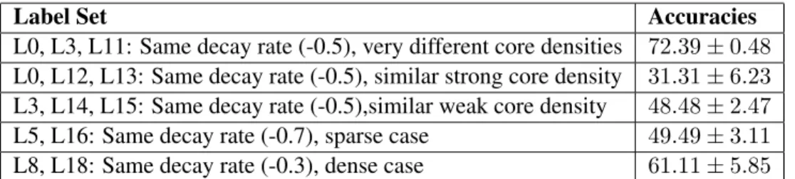
L0, L3, L11: Same decay rate (-0.5), very different core densities 72.39±0.48 L0, L12, L13: Same decay rate (-0.5), similar strong core density 31.31±6.23 L3, L14, L15: Same decay rate (-0.5),similar weak core density 48.48±2.47 L5, L16: Same decay rate (-0.7), sparse case 49.49±3.11 L8, L18: Same decay rate (-0.3), dense case 61.11±5.85

(35)

2.5.2 Classification graphs of the same type, where each label corresponds to a prob-ability matrix with different parameter values.

As in subsection 2.5.1, in all cases one can observe substantial gains in classification accuracy on the held-out test sets when compared to classification on a flattened adjacency matrix feature space. As also observed in subsection 2.5.1, some within-experiment accuracy scores maintained their relative positions while others did not. The scenario where an accuracy remains the highest when compared to other experiments is most clearly apparent for the experiments in using ordered graphs (tables 2.9 and 2.15). In other cases, the pattern does not quite hold. Consider tables 2.14 and 2.8. When using flattened adjacency matrices as a feature space, random forests struggled the most when tasked with classifying graphs displaying a spectrum of edge-probabilities. However, when using network statistics, random forests yielded lower classification accuracy scores for the experiment comparing relatively sparse graphs than when discriminating on a spectrum of edge-probabilities.

Similar comparisons can be made for all the relevant tables, with the most relevant conclusion being that, for all cases, the use of network statistics as a feature space results in large gains with respect to classification accuracy. In many cases, under network statistics, random forests achieved perfect discriminatory power. Interestingly, whether the relative changes in accuracy across sub-experiments mirrors those displaced in the flattened adjacency cases seems to depend on graph type and the set of graphs random forests is tasked with classifying.

2.6 Summary

(36)

0 25 50 75 100

Random Assortative Disassortative Ordered Core−periphery

Graph Type

Accur

acy (%)

Feature Space Flattened Adjacency Matrices

Network Statistics

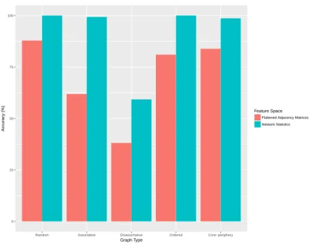
Figure 2.2: Summary of Classification Accuracies when Varying Number of Communities.

Results from tables 2.7 and 2.13.

Recall that sets of experiments in sections 2.3.2 and 2.5.1 examined random forests’ discrimina-tory power when classifying between models of the same type (i.e. random, assortative, disassortative, ordered, and core-periphery) with the same numbers of nodes and general parameters in the prob-ability matrix. The only differences between these models was the number of communities. As seen in figure 2.2 not only did the use of network statistics result in substantial gains for all graph types, the relative accuracies between graph types was also approximately the same. In other words, classifiers on the flattened adjacency matrix space that performed better for a given graph type versus a different graph type still performed better for the given graph type when trained on the network statistics space.

The second set of experiments (sections 2.3.3 and 2.5.2) examined the discriminatory power of random forests when graph types are the same with same numbers of communities and nodes, but with different underlying edge probabilities. As noted before, when using network statistics as a feature set, the discriminatory power of random forests substantially increases. In many cases random forests achieved perfect classification accuracy scores. Interestingly, the relative change in accuracy when using network statistics as opposed to flattened adjacency matrices as a feature space does not necessarily remain the same as it did for figure 2.2. For example, consider the results

(37)

0 25 50 75 100

dense comparison sparse comparison spectrum

Accur

acy (%)

Flattened Adjacency Space

0 25 50 75 100

dense comparison sparse comparison spectrum

GraphType

Assortative

Random Network Statistics Space

0 25 50 75 100

dense comparison L0:L2 sparse comparison spectrum

Accur acy (%) 0 25 50 75 100

dense comparison L0:L2 sparse comparison spectrum

GraphType

Disassortative

Ordered

Figure 2.3: Summary of Classification Accuracies when Varying SBM Probability Matrices.

Results from tables 2.8, 2.9, 2.14, & 2.15. The lefthand column summarizes random forest classifica-tion accuracies on the flattened adjacency matrix feature space for experiments using all graph types, excluding core-periphery graphs. The righthand column does the same for the network statistics feature space.

for assortative and random graphs shown in the top row of figure 2.3. When trained on flattened adjacency matrices, random forests had better overall accuracy in discriminating different instances of random graphs than when classifying different assortative graphs. However, when using network statistics as a feature space, higher classification rates occur for the assortative graphs. This trend reversal also occurs when comparing disassortative and ordered graphs (second row of figure 2.3).

(38)

0 25 50 75 100

L0 − L2 L0 & L6 L3 − L5 L3 & L7

Accur

acy (%)

Core−Periphery, Exp. 1

0 25 50 75 100

L3 & L10 L8 & L9

Accur

acy (%)

0 25 50 75 100

L0, L12, L13 L0, L3, L11 L3, L14, L15 L5, L16 L8, L18 Label Set

Accur

acy (%)

Figure 2.4: Summary of Classification Accuracies when Varying SBM Probability Matrices (core-periphery graphs).Results from tables providing accuracy scores from both feature spaces for the sub-experiments using core-periphery graph types. Red columns correspond to results from classifiers trained on the flattened adjacency matrix feature space, blue columns correspond to those trained on the network statistics feature space.

(39)

CHAPTER 3

Model Selection Using Random Forests

This chapter explores the question posed at the beginning of this thesis: givenN candidate stochastic block models for a particular networks data set, is it possible for a random forests classifier trained on a set of instance graphs generated from theseN SBMs to select the best fit to a real-world network? Our goal is to determine whether this well-known and relatively easy to implement machine-learning classification technique can serve as a comparable method for fitting generative models to a given network’s physical and probabilistic structure. We have divided this chapter into two sections. The first provides an overview of the tools and techniques used to determine theN candidate models. This section also describes the real data set used for our experiments. The final section presents our findings in comparing the model selected by random forest to the “gold standard” model selected using the criteria described below.

3.1 Overview of the

R

package ‘mixer’and data set

(40)

Figure 3.1:Summary of Mixer Models fitted to the Macaque data set.Top left: ICL vs number of communities per model. The dotted red line indicates that the 4-community MixNet model maximizes ICL and is therefore the best fit to the macaque data set. This model serves as thegold standardwith which to compare the our own “best model” chosen by random forests. Top right: Adjacency matrix organized under the best model. Bottom left: Degree distribution. Bottom right: Schematic of probability strength between and within communities under the best model.

resulting in a pattern strongly reminiscent of the assortative graph structure. Using mixer, the process of fitting several MixNets of differing numbers of communities to the macaque data set is trivialized to a few lines of code and has the additional benefit of allowing us to choose in advance a gold standard with which to compare our random forests results. As shown in figure 3.1, we shall assume that the best model for our data set has 4 communities.

3.1.1 Brief overview of MixNet models

This section provides a brief summary of previous work that derived the tools and methods used to define our set ofN models for the macaque data set. A detailed description for the derivation, properties, parameter estimation techniques, and model selection criteria of the Erd˝os-R´enyi mixture

(41)

for random graphs can be found in Daudin et al. (2008) and information regarding ICL is presented in Biernacki et al. (2000).

In defining MixNet, Daudin et al. (2008) assumes the mixture model framework for defining the underlying probabilistic structure of a given network. Note that the SBMs presented in section 2.1 are all mixture models and thus are a reflection of the same framework about to be described. Paraphrasing the notation in Daudin et al. (2008), mixture models assume nodes are grouped into Kcommunities with prior probabilityαk. Let{Zik}be an indicator variable for the community of nodei, then the prior probabilities of node-community membership can be expressed as

αk=P r{Zik = 1}, with

X

k

Zik = 1,

X

k

αk= 1 (3.1)

Recall that setting edge-probabilities asP(Aij = 1)∼Bernoulli(p)produces the so-called Erd˝os-R´enyi random graph model, G(n, p). Rather than assuming that edges are independent with Bernoulli(p)distributions, Daudin et al. (2008) requires the definition of inter-community probabili-tiesπkl, or the probability that a node in communitykconnects to a different node in communityl. As in the cases outlined in section 2.1, graphs are assumed to be undirected, which means thatπkl =πlk. Finally, edges in these graphs are assumed to be conditionally independent of the communities involved and no self-loops are allowed,



 

 

Aij|{Zik = 1, Zjl= 1} ∼Bernoulli(πkl) Aii= 0

(3.2)

The connectivity matrixπππ= (πkl)in Daudin et al. (2008) is the same as our own probability matrix M defined in section 2.1.

3.1.2 MixNet model estimation

(42)

To begin, Daudin et al. (2008) defines the log-likelihood of a network defined under the MixNet model as

logL(X,Z) =X i

X

k

Ziklogαk+ 1 2

X

i6=j

X

k,l

ZikZjklogBernoulli(Xij;πkl) (3.3)

whereX ={Xij}is the set of all edges andZ ={Zik}is the set of all indicator variables defined previously. Note that Bernoulli(X;π) =πX(1−π)1−X. As discussed in the literature, the likelihood

L(X)cannot be simplified into a more tractable form for computation. Instead, Daudin et al. (2008)

proposes a variational approach that attempts to optimize the lower-bound of the likelihood function and an iterative algorithm designed to estimate the prior probabilitiesαααand the class-connectivity matrixπππwhile maximizing this lower bound. This algorithm assumes a fixed number of communities K when updating the parametersαααandπππ. To choose the best model given differentK, Daudin et al. (2008) uses a modified Integrated Classification Likelihood selection criterion developed by Biernacki et al. (2000). Given a modelmK ofK communities, this model selection criterion is defined as

ICL(mK) = max

θθθ logL(X,

e

Z|θθθ, mK)− 1 2×

K(K+ 1) 2 log

n(n−1)

2 −

K−1

2 logn (3.4)

whereθθθ= (ααα, ππ)π is the entire set of mixture parameters,Zeare the predictions ofZ, andnis the

total number of nodes in the model (Daudin et al., 2008). The Rmixer()function implements these equations on a given adjacency matrix for a pre-defined range ofK. For each of theKmodels, equation 3.4 is computed. The model with the largest ICL value is selected as the best fit to the data (see panel 1 in figure 3.1).

3.2 Model Selection using Random Forests

Using the tools described in section 3.1, we are now able to examine random forests’ effectiveness as a model selection criterion for the macaque data set. Following the workflow defined in figure 1.1 for real data sets, we specified the following binary classification problem using the tools described in section 3.1. SBMs of 4 and 5 communities were estimated on the macaque data set (see figure 3.2

(43)

MixNet Average Density

k= 4 0.2899 k= 5 0.2886

Table 3.1: Average Densities of 4- and 5-Block MixNet Realizations. As reflected in this table, the models fitted to the macaque data set produce graphs of roughly the same density. In this case, the average densities over all realizations used for this experiment are shown. Intuitively, one may expect any classifier to perform poorly once graphs achieve a certain level of similarity with respect to their densities, particularly if one notices that many of our features in section 2.4.1 are closely related to graph density. However, as shown in Caceres et al. (2016) and later in this section, random forests discriminatory power remains quite strong as long as the underlying edge-probabilities remain relatively distinct.

and table 3.1) with 100 graph realizations generated from each model, to be used as a train/test set. Additionally, we also generated another data set in the same manner for use as a further test set. Each graph realization was assigned a label corresponding to the number of communities of the parent SBM. Both the flattened adjacency matrices and the list of network statistics (section 2.4.1) were extracted from the realization data sets as well as the original data as separate feature sets.

To test random forests’ ability to select the best generative model for this data set, (where “best” is assumed to be the 4-community model that maximizes the modified ICL criterion), individual forests of5,10,15, ...,150trees were constructed. Each forest was fit using 10-fold stratified cross-validation and the classification accuracy scores were averaged over the held-out test sets and again over the additional set of 200 different instance graphs. The classifiers were additionally tasked to select one of the SBMs as a fit for the original data set, receiving a score of1if correctly matching the original data set to the 4-block SBM and receiving a0otherwise. This process was repeated 100 times for each given number of trees and the final accuracy scores were recorded as averages across these 100 iterations. The entire experiment was conducted first using the flattened adjacency matrices as a feature set, then using network statistics.

3.2.1 Model selection with edge-based classification

(44)

Figure 3.2: Adjacency Matrices of Original Macaque Data with 4- and 5-Block Realizations.

Using the methods described in section 3.1, SBMs of 4 and 5 blocks were estimated for the macaque data set. The original adjacency matrix (left) and two realizations of the 4- and 5-block models (top and bottom) are shown.

the original data set with the gold standard 4-community model. As the classifier grew in number of trees, becoming more and more adept at discriminating between the instances of the 4- and 5-block models, the chance of selecting the gold standard model became practically zero.

3.2.2 Model selection with network statistics-based classification

From the perspective of network statistics, random forests did less well in classifying realizations of the 4- and 5-block SBMs but vastly out-performed random forests trained on the flattened adjacency feature space as a model selection criterion. As the number of trees per classifier grew, these models not only became more adept in classifying graph realizations, they also began to consistently match the original data set to the same 4-community model chosen by ICL model selection criteria.

3.2.3 Results

The results for this experiment are summarized in figure 3.3. The green lines, corresponding to “test set 1,” represent classification accuracy on the held-out test sets during stratified 10-fold

cross-validation. The blue lines for “test set 2” represent classification accuracy on the separate,N = 200

(45)

data set. This serves as an additional check on the behavior of random forests by using a “new” data set that was not used in the training/testing phase. Recall that both test sets 1 and 2 consist entirely of instance graphs generated from the 4- and 5- block SBMs. Finally, the red lines represent how often a random forests classifier on a given feature space and number of trees matched the original data set with the gold standard 4-community SBM. In the framework of this experiment, these curves can be interpreted as a rough proportion of the frequency (out of 100) with which the given classifier chooses the optimal model maximizing the ICL criterion in section 3.1.2. Our best random forests model selection criteria was the 140 tree model trained using network statistics, which chose the gold standard model approximately 97 times out of 100. In contrast, the best random forests classifier using flattened adjacency matrices selected the gold standard model for the macaque data set only 28 times out of 100 using 10 trees. Interestingly, strong performance as a model selection criteria does not seem to necessarily translate into strong discriminatory power between graph realizations of the 4- and 5- block SBMs. As seen in the blue and green curves in the lefthand plot, the edge-based classifiers achieve perfect discriminatory power between graph realizations usingnT rees > 50. However, network statistics-based classifiers never achieve perfect discriminatory power with respect to the instance graphs, achieving an average accuracy of at most around87.14%fornT rees= 135.

(46)

Figure 3.3:Random Forests as a Model Selection Criterion.Left: Classification accuracy versus number of trees for random forests modeled on flattened adjacency matrices of the instance graphs and original data set. Right: Classification accuracy versus number of trees for random forests modeled on network statistics (section 2.4.1) of the instance graphs and original data set. For both plots smoothed lines of fit are given, with grey areas representing standard error.

(47)

CHAPTER 4

Conclusion and Future Directions

In this thesis, we have outlined a series of experiments that explores random forests’ dis-criminatory power over an extensive range of Stochastic Block Model parameters and structural configurations. To provide further comparison, we implemented these experiments using two differ-ent feature spaces, the first taking advantage of the trivial form of connectivity information encoded in raw edge-weights of the graphs - our so-called “flattened adjacency matrix feature space” - the second building off of previous research in network classification by using an extensive list of network statistics. These network statistics can be loosely grouped into measurements related to node degree and graph connectivity, information about shortest paths, and linear algebra concepts using the graphs’ adjacency matrices. Overall, classifiers trained on a network statistics feature space not only vastly outperformed those trained on the flattened adjacency feature space, but also generally achieved high rates of classification accuracy. While this is perhaps not a difficult conclusion to comprehend, knowing beforehand that one can expect good discriminatory power in reasonable network classification scenarios by using random forests and network statistics can be extremely helpful to researchers needing fast, easily interpretable results when classifying networks.