1176.pdf

KEVIN M. BOYLE. Numerical Calculation of Aspiration

Efficiency of Aerosols into Thin Walled Sampling Inlets

(Under The Direction of Dr. MICHAEL R. FLYNN)

Aspiration efficiency of particles from a flowing

airstream into a thin walled sampling inlet is accurately

predicted using a numerical model. The model combines the

Boundary Integral Equation Method for predicting the

velocity field into the inlet with an analytical solution to

the particle equations of motion. A two and a three

dimensional model are examined. Results for the three

dimensional model correlate well with an empirical model of

aspiration efficiency. The method can be generalized to a

wide range of airstream, sampling inlet, and particle

I . BACKGROUND...1

11 . THEORY...7

III. METHOD...13

IV. RESULTS...31

V, DISCUSSION...39

VI. CONCLUSION...48

VII. FUTURE WORK...49

VIII. APPENDIX...53

IX. REFERENCES...118

I would like to thank Dr. Michael R. Flynn, Department

of Environmental Sciences and Engineering, for his guidance

and constant encouragement throughout the course of this

project. I am also grateful to Dr. David Leith and Dr.

Russell W. Wiener for their comments and suggestions

regarding the content and preparation of this report.

I extend my sincerest appreciation to my wife, Ellen,

and daughter, Sarah, for their understanding and support

throughout this project.

I would also like to thank the United States Air Force

for providing the opportunity and financial support needed

to complete my program of study.

This research was funded by the U.S. Environmental

Protection Agency under grant NO. 44213.

AEROSOLS INTO THIN-WALLED SAMPLING INLETS

by

Kevin M. Boyle

Unbiased sampling of airborne particulate from a

flowing stream requires that the size distribution and

concentration of aerosol collected be identical to that of

the aerosol in the free stream. Sampling errors occur

during aspiration of the aerosol from the free stream to the

face of the inlet and during transmission of the aerosol

along the sample tube. Additional losses or gains may occur

due to particle bounce from the front edge of the sample

tube. In this paper, a numerical model for determining the

aspiration component of overall sampling efficiency for any

arbitrarily shaped thin edged inlet is presented.

BACKGROUND

Sampling errors due to aspiration occur when particles

fail to enter the sampling inlet with the air. Particles

have inertia which may prevent them from accelerating,

decelerating, or changing their direction fast enough to

move with the air (Agarwal and Liu, 1980). Particles also

possess additional motion due to gravity. Aerosol

location, Co, (Belyaev and Levin, 1972).

Ea = Ci (1)

Co

One effect on aspiration efficiency would be loss or

gains of particles due to bounce off the front of the

sampling inlet. By modeling the system as a thin walled

sampling inlet, particle rebound effects are assumed

negligible and do not contribute to the overall aspiration

efficiency (Belyaev and Levin, 1974).

Both numerical modeling and physical experiments have

attempted to describe aspiration efficiency. Belyaev and

Levin (1972, 1974) used flash illumination to photograph

particle trajectories and develop equations to predict

inertial aspiration efficiency. Durham and Lundgren (1980),

developed aspiration equations from experimental data for

aspiration efficiency during anisokinetic sampling with

nozzle misalingment and sampler inlet velocity different

from oncoming wind velocity. Their equations account for

the projected area of the nozzle when it is misaligned.

Jaysekera and Davies (1980) and Davies and Subari (1982)

also performed experiments and derived aspiration equations

which were similar to the equations of Belyaev and Levin.

Extensive measurements of sampling efficiency were made

by Tufto and Will eke (1982), and Okazaki, Wiener, and

non-and work cited above, Hangal non-and Willeke (1990) proposed a

unified model to predict aspiration efficiency, Ea. The

general expression , equation(2), is:

Ea = 1 + (R cos e - l)f (2)

where R is the velocity ratio, e is the sampling angle and f

is an inertial parameter. For the case of 0° sampling angle

the inertial parameter, f, is based on the work of Belyaev

and Levin (1974) and is shown in equation (3).

f = 1 - 1 /[I + (2 + 0.617/R) Stk] (3)

R = Uo/Ui

Uo is the free stream velocity

Ui is the inlet velocity

Stk is the Stokes number

For C to 60° sampling angle the parameter is based

on the work of Durham and Lundgren (1980), equation (4).

f = [1 -1/[1 +(2 + 0.617/R)stk']]

[1 - 1/[1 + 0.55stk' exp(0.25stk')]3/

[1 - 1/[1 + (2.617)stk']] (4)

where

stk- = Stk exp (0.0226) (5)

To model the movement of particles in air it is

trajectory paths have been developed by Agarwal and Liu

(1980), Addlesee (1980), and Dunnett and Ingham (1986,

1988). Agarwal and Liu determined the theoretical flow field

into a thin walled sampling inlet considering both particle

inertia and gravitational settling. A numerical calculation

procedure was used to solve the axisymmetric Navier-Stokes

equations and particle motion equations.

Addlesee, (1980) studied the intake efficiency of a

Case11a cascade impactor. The impactor was modeled as a two

dimensional infinite slot with no end effects. A solution

to the flow field was developed by assuming that viscous

forces were not significant and calculating stream lines

using potential theory. From the flow field developed, the

particle equations of motion were solved assuming that

Stokes law is applicable (Re < 1). The equations were put

into finite difference form and solved by relaxation.

Dunnett and Ingham (1986) developed a mathematical

theory to predict aspiration efficiency of two dimensional

blunt bodies using the Boundary Integral Equation Method.

Once the velocity field of the system was known, the

particle equations of motion are solved assuming that the

Reynolds number is always less than 1.0 and thus Stokes'

drag could be applied. The equations were put in finite

difference form and solved numerically. In 1988 they

expanded the two dimensional solution to an axisymmetric

techniques.

Flynn and Miller (1989) used the boundary integral

equation method to model air flow into local exhaust hoods.

Their solutions follow the same logic as Dunnett and Ingham

and give good agreement with analytic solutions for flow

into an infinitely flanged rectangular hood with a constant

velocity at the hood face, and with other empirical models.

The advantage of their model was that it reduced a 3

dimensional air flow solution to a 2D area solution along

the boundary of a specified domain.

This research employs the model of Flynn and Miller to

estimate the air flow into a sampler inlet, and then applies

the solution for the particle equations of motion developed

by Alenius (1989) to determine aspiration efficiency. The

particle motion equations are described in the THEORY

section which follows.

The referenced numerical models to calculate aspiration

efficiency were limited by the geometry of the solution

domain and employed finite difference techniques to solve

the particle equations of motion. By combining the 3D

airflow solution of Flynn and Miller with the analytic

solution to the equations of motion proposed by Alenius

domain and sampling inlet over a wide range of particle size

To model particle flow, a method for determining the

characteristics of the flow field into an arbitrarily shaped

and oriented sampling inlet is required. Once the flow

field is described, particles can be placed into the field,

assigned initial conditions, and tracked. From the

trajectories, an estimate of the aspiration efficiency can

be made and compared with previous models or experimental

data.

The boundary integral equation method (BIEM) is a

method of solving a potential flow problem for any

arbitrarily shaped domain. The assumptions in the

development are inviscid, incompressible, irrotational flow

which leads to the following expressions:

grad-V = 0 (continuity equation for (6)

incompressible flow ),

and;

curl V = 0 (irrotational flow). (7)

Irrotational vector fields possess a potential function such

that the vector is equal to the gradient of the potential,

<t), and thus

V = grad 0. (8)

By combining the above equations

grad-V = grad-(grad <t>) or

Equation (9) is Laplace's equation. By applying the

divergence theorem and Green's second identity, an equation

can be derived which relates the velocity potential an any

singular point (P) to the potential and normal derivatives

of potential along the boundary of a specified domain.

The derivation (Liggett and Liu, 1983) yields the

following equations which form the basis of the Boundary

Integral Equation Method for two and three dimensional

2D: a<t>(T) = Sr [((fl>/R) 6R/6n) - ((InR) 60/6n)] dS (10)

3D: -a0(P) = Ss [(0(6(1/R)/6n)) - ((l/R)60/6n)] dA (11)

0 = velocity potential

60/6n = velocity normal to the boundary

a = solid angle about (P)

R = distance from singular point (P) to

a point on the boundary,

r = closed curve surrounding and defining

the 2D domain

SI = closed surface surrounding and defining

the 3D domain

dS = differential element on r

dA = differential area on S.

The above equations can be written in discrete form in

either two (Liggett and Liu, 1983) or three dimensions

(Flynn and Miller, 1989). After specifying either <t> or

6*/6n at each node on a discretized boundary of N nodes,

equation (10) or (11) is written for each node by

boundary values are known, (P) can be located at any

internal location and the left hand side of equation (10) or

(11) differentiated to give the velocity at the internal

point.

Once the velocity field is determined, particles can

be placed in the air stream and their motion tracked. This

model uses an analytical solution to the particle equations

of motion developed by Alenius (1989). The general form of

.the equation is:

d2r/dt2 - [Q(Re)/T(u-(dr/dt))]-g = 0 (12)

where bold face variables denote vector quantities.

In the above equation, the following notation is used:

d2r/dt2 (=dv/dt) is the acceleration of the particle

Q(Re) is a dimensionless factor based on the

Reynolds number and the drag

T is the particle relaxation time in air

u is the air velocity at the particle

location

dr/dt=v is the velocity of the particle

g is the earth's gravity

0 is the null vector

r is the particle position vector

velocity u vary along the trajectory of the particle and

thus indirectly with time t. If the air velocity at the

points where the particle is successively located can be

described as a linear function of the time that has elapsed

and Q(Re) is assumed to be constant over the time interval,

an analytical solution to the general equation can be

obtained. This condition is approximately met if the motion

of the particle is successively calculated using

sufficiently small time intervals. A complete derivation is

presented in the appendix. The analytic solution is:

v(t-ff) = Uat'+Ub-(Ub-v(t))exp-[Q(Re)t'/T] (13)

r(t+t') = r(t)+Ua/2t'2+Ubt'

-(Ub-v(t))T/Q(Re)(l-expQ(Re)tVT) (14)

where t' is the size of the time step and Ua and Ub have

been added to simplify the appearance of the equation:

Ua = (u(t) -u(t-t'))/t' (15)

Ub = u(t)-(Ua-g)T/Q(Re). (16)

Particles can now be tracked in any domain in which the

air field is known, and the efficiency of aspiration

determined. Aspiration efficiency is calculated as the

ratio of particles entering the inlet to particles in the

undisturbed flow field far upstream, equation (1). Figure 1

Freestream

Critical

Trajectory

SAiyiPLiNG INLET

Co Uo Ao = CI Ul Al

Fiaure 1. Conceptual Stream Tube. The flux of Pa»^i°l«^^^

th?ough the upst?eam plane equals that of particles passing

airstream of given velocity, Uo, into an inlet sampling at a

constant velocity, Ui. The boundaries of the stream tube

represent all particle trajectories which just enter the

tube. These trajectories are called critical trajectories.

Particles located outside this tube would not be drawn into

the inlet. The flux of particles passing through the

upstream plane of the stream tube is particle concentration,

Co, multiplied by the stream tube cross sectional area, Ao,

times the freestream velocity, Uo. By

equating the flux of particles through the plane of the

stream tube upstream from the inlet to that through the

plane of the sampler face, Ci Ai Ui, the expression in

equation (17) is obtained.

Co Ao Uo = Ci Ai Ui (17)

From equation (1), Ea = Ci/Co, thus:

Ea = Ao Uo/Ai Ui (IB)

In equation (18), the characteristics of the sampler

inlet, Ai and Ui, are known as well as the free stream

velocity, Uo. By determining the coordinates of the

critical trajectory start points in the free stream, an

estimate of Ao and Ea can be made. This can be done by

iteratively assigning particle locations in the free stream

and tracking each particle in the domain until the critical

METHOD

The model was developed using a simple two dimensional

problem which was then expanded to a more complex three

dimensional case. Both isoaxial and non-isoaxial inlet

orientations were modeled. Non-isoaxial conditions

consisted of orienting the inlet at a pitch angle of 30° to

the freestream.

Two Dimensional Model

The two dimensional problem was modeled as an infinite

slot. The coordinate system to visualize in two dimensions

is an x-y cartesian system with the origin located at the

center of the inlet. The positive x direction extends along

the centerline of the hood face and the y direction is up

and down, with gravity acting in the -y direction.

The air flow into the slot was modeled using the

boundary integral equation method which provided a solution

everywhere on the boundary of the domain for the potential

and the normal derivative of potential. From the boundary

solution, the exact velocity components at any internal

point were calculated.

A FORTRAN computer program for the two dimensional

boundary integral equation solution, written by Liggett and

Liu (1983), was used for the 2D solution. The program,

called GM8, returned the boundary values and the local air

velocity components within the domain needed to calculate

written to solve the Alenius solution to the equations of

motion, (11) and (12), and track particles within the

domain. Figure 2 shows the flow of logic in the program.

The boundary of the domain in the simple 2-D case is

shown in figure 3. The origin of the coordinate axes are

located at the center of the sampling inlet. The upper

lower, front and rear boundaries of the domain are at a

distance of 20 inlet diameters from the inlet face. The

remaining boundary consists of a rectangular indentation to

represent the sampling nozzle of diameter equal to its

width.

In figure 3, the boundary conditions are marked. The

upper, lower, and rear boundary are situated far enough away

from the sampling inlet to have potential due exclusively to

the free stream velocity, or:

0 = Uox(x) + Uoy(y) (19)

where Uox and Uoy are the magnitude of the free stream

velocity components and x,y are the location coordinates.

The boundary condition on the line opposite the hood face is

60\6n = Uox, the free stream velocity normal to the surface.

On the upper and lower edges of the sampling inlet the

boundary conditions are 60\6n = 0, no flow through the walls

of the nozzle. At the face of the inlet 60\6n is equal to

sampling velocity, Ui.

For the situation where an inlet pitch angle was

( START ;

I S«tecttni|ectorY

"^ starling coordinates

Calculate air velocity

at particle location

! using BIEM

Predict particie |

after time step, f !

,.. Test lor

trajectory end

,''Test for

convergence

/ Output critical /

, trajectories j

STOP

Figure 2. Flow diagram for the two dimension and 3

^s Uox(iO

+ Uoy(y)

Uox(x)

+ Uoy(y)

^ = Uox(x) + Uoy(y)

ͣ

---•---•---•—'---•

Y 1

6^/6n s 0

X i

6^l6n s 0

• •

i---•---1

• anodes

1---

ͣ

---i

6^/in

4 =Uox

^ = Uox(x) •<- Uoy(y)

Figtire 3. 2D model boundary with coordinate axes, boundary

condtions, and ssunple discretization shown. 0 = potential,

boundary calculated. Rather boundary conditions were

adjusted to represent the freestream, Uo, as

the resultant of the free stream normal to the front

boundary, Uox, and a crossdraft, Uoy. This required a

coordinate system conversion where the gravity vector in the

X and y direction were -g sin(e) and -g cos(e) respectively,

e was the angle of misalignment and g the magnitude of the

gravity vector. The origin of this coordinate system was

still centered at the inlet face.

The solution required the domain to be discretized into

nodal elements as shown in figure 3. Much finer

discretization than presented in the example is required

because numerical accuracy during calculation of internal

points suffers when the internal point is within 1 element

length of the boundary.

The initial conditions assigned to the particles in the

free stream are that they are falling at their terminal

settling velocities and moving in the air stream (Addlesee,

1980) at the velocities calculated by the BIEM solution.

Terminal settling velocity (Vts) was calculated using

Vts = T g (20)

where t is the particle relaxation time (Reist, 1984) and g

is the acceleration due to gravity.

In two dimensions, it was necessary to define the

critical trajectories to calculate aspiration efficiencies.

This is because in two dimensions equation (18) reduces to:

Ea = do Uo/di Ui (21)

where di is the inlet diameter, and do is the distance

between the upper and lower critical trajectories. Internal

air velocity coordinates were calculated using BIEM, then

the particle position and velocity were predicted using the

analytical solution and the process repeated. The critical

trajectories were determined by selecting a point far

upstream and tracking a particle from this point either into

(capture) or past (miss) the inlet. Once a missed and

captured trajectory were found the average of the two

starting points determined the next point. Convergence

occurred when the distance between the particle trajectory

start point which is captured and that which escapes is less

than a preset value. The program was designed to locate

both an upper and lower critical trajectory corresponding to

the upper and lower edges of the sampling inlet. The

distance, s, between the upper and lower critical

trajectories, do, was determined using the distance formula,

equation (22).

S = ((Xl-X2)2 + (yi-y2)2 + (21-22)2)54 (22)

Three Dimensional Model

In three dimensions, Uo, Ai, and Ui are given and Ac is

determined to calculate aspiration efficiency, equation

(18). Ao is the area of the trajectory tube at an upstream

sampling velocity. This area represents the boundary of the

stream tube at an upstream location in which particles will

enter the sampling inlet (Fig 1).

The shape of the three-dimensional domain is a square

sided volume of half-width equal to 20 inlet widths.

Extending from the rear wall of the volume into the center

of the volume for a distance of 20 inlet widths is a

sampling inlet with a square cross section. An equal area

square is used to model a circular inlet to simplify the 3D

boundary discretization.. The origin of the cartesian

coordinate system is located at the center of the inlet.

The X direction extends away from the hood face along its

centerline. The z coordinate represents the height of the

domain and the y coordinate represents the width.

For boundary conditions, the potential is specified on

the front, rear, top, bottom and side faces of the 3D

domain. The velocity is specified over the inlet face as

Ui, and at the walls of the inlet tube as 0 cm/sec. As in

2D, the boundaries of the 3D domain are situated far enough

away from the inlet to have potential due exclusively to the

0 = Uox(x) + Uoz(z) (23)

Here, Uox represents the velocity perpendicular to the front

face of the domain and Uoz is the crossdraft vector used

when the sampling angle did not equal zero. As in 2D, the

gravity components in the coordinate system must be adjusted

The flow field is defined using the same theory as in

two dimensions but using a FORTRAN program written by Flynn

and Miller (1989) to solve the BIEM problem for three

dimensions.

Particle trajectories were calculated in the same

manner as in two dimensions with BIEM providing the local

air velocity components at the particle location. The

particles were assigned initial conditions as described in

the 2D section and the equations of motion, with a third

dimension added, were solved to predict the particle's next

position and velocity. The program logic is the same as

that shown in figure 2.

Because the domain is now in three dimensions, the

region cannot be discretized into lines between nodes,

rather, the boundary must be divided into areas. Flynn and

Miller (1989) used triangular elements on the boundary.

Examples of the discretization input files for the boundary

are presented in the appendix.

The critical trajectories in 3D were determined by

selecting a point far upstream and tracking a particle from

this point either into the inlet (capture) or out of the

domain (miss). The start point is a specified number of

inlet diameters, XDIN, in front of the inlet and in the

direction of the resultant velocity vector in the x-z plane.

For 0", this point is along the x axis at x=XDIN, y=0, z=0,

the first trajectory start point, figure 4, is calculated

as:

X = XDIN cos(e)

y = 0.0 (24)

z = XDIN sinO)

The rationale for choosing this start point is to

obtain a capture trajectory around which starting points for

the critical trajectories can be centered. If this first

point does not yield a capture, the start point is

incrementally adjusted up or down along a line perpendicular

to the free stream and the trajectory is recalculated. The

process is repeated until a first capture identified.

Once a capture trajectory is found, a series of start

points at which to begin critical trajectories are defined

at a distance far enough away from the coordinates of the

first capture to have a high probability of a miss. These

points are located a specified distance, AA, from the

coordinates of the first capture (xl,yl,zl) in incremental

degree steps, a, around a semicircle in the plane

perpendicular to the free stream, figure 5. Critical

trajectories for only one half the area were calculated due

to the symmetry of the problem.

The equations for these points are:

X = xl + (AA sin(e) sin(a))

LlM 0) pMn* ptrpwdlculr

lefiMitrtMn.Uo

X1 B XDtN COS(e)

Y1 = 0.0

Z1=XDINSIN(e}

Figure 4. Location of initial trajectory start point.

(X1,Y1,21) is initially placed at a distance XDIN in front

of the inlet along a line perpencular to Uo in the X-Z

{x1,y1,z1)

^

Trajectory start points

x = x1 + (AAsJn(0)sln(a))

y = AA cos(a)

z = z1 + (AA cos(0) sin(a))

0 = angle of misalignment

Figure 5. Trajectory start points are located on a

semicircle centered around (X1,Y1,Z1) at degree increments,

a, along rays a distance AA from the center.

If the start points defined in equation (25) result in

a capture, the start point is incrementally adjusted farther

from the initial capture point and the trajectory is

recalculated until a miss identified.

Each first capture and initial miss coordinate

combination results in a ray the end points of which define

the upper and lower bounds of the critical trajectory and

all rays are contained in the same plane perpendicular to

the free stream. From this point, the starting coordinates

of the last miss and last capture trajectory are averaged to

determine the coordinates of the next start point on the

ray. The process is repeated until the convergence criteria

was satisfied. Critical trajectories are found for each

starting point around the semicircle.

The output of the particle tracking routine is a series

of points representing the critical trajectories which

define Ao. The area, Ao, is calculated numerically with a

FORTRAN program using the trapezoid rule. From Ao, Ea is

calculated using equation (18).

The models, both 2D and 3D, were verified by comparing

the computed aspiration efficiency with the unified

aspiration model proposed by Hangal and Willeke (1990),

equation (2).

The Programs

The two dimensional program was compiled and run using

Microsoft Fortran version 2. The entire aspiration

program initially calculates the boundary solution for the

domain then calls subroutines to calculate particle velocity

and position, and internal air velocity components at the

particle's location. All 2D simulations were run on a Dell

386 personal computer and took approximately 15 minutes to

complete. Each program run calculates approximately 30

separate trajectories with approximately 100 points

calculated per trajectory.

Figure 6 shows an example of the output of the 2D

program with particle positions plotted as trajectories.

The particle trajectories were plotted using a simple

routine written in BASIC (see appendix). The distance

between the upper and lower critical trajectories was the

basis of determining the aspiration efficiency as defined in

equation (22). A commented version of the 2D program is

contained in the appendix.

The 3D program is much more complex than the 2D version

because of the addition of a third dimension and the

resulting complexities of solving the BIEM equations.

Because of this, 3D simulations were run on a Convex Super

Computer. The 3D simulations were run using two FORTRAN

programs. The first program, 4PTGQ.F, is the BIEM boundary

solution program. The input for this program was a boundary

node and element file for each combination of sampling

velocity, Ui, wind velocity, Uo, and sampling angle, 6. The

input file contained 367 nodes, N, leading to N linear

• iiHiin'.- ... .iii.iii.-."..'...;j!

ͣ

]:,

ͣ

;;,...; ;''"'":'

ͣ

'.'''-1 ͣͣ-.,,ͣ.-v,,.:

ͣ

/*.•. ͣ'. '''ͣͣͣ:

EFF = "'^012572 %>

ͣ

UO = -250 -... %•

DP = .0005 %:

-DIN = 1 %^:

THETA = 29.9991 •. ^

UI = 1000

Figure 6. Sample of 2D trajectory plots. Trajectories

originate in the plane of the freestream perpendicular to

point gaussian quadrature. This program took 5.5 minutes to

run on the Convex and returned potential and velocity values

for each node on the boundary of the domain.

Once the output to 4PTGQ.F was received, it was

imported as input to the 3D particle tracking program,

TRK15.F. This program consists of a driver to specify

particle location, test for convergence, and call

subroutines to perform the BIEM internal air velocity,

particle position, and particle velocity calculations.

TRK15.F was designed to calculate 13 trajectories at 15° (a

= 15° in equationkk (25)) increments around a semicircle

surrounding the initial capture point (see figure 5). This

leads to the calculation of approximately 10 trajectories

per starting point, over the 13 starting points specified by

the degree increment, a, with 20-30 points along each

trajectory to determine the fate of the particle. A typical

combination of program variables shown below took 68 minutes

of computer time on the Convex:

Uo = 500 cm/sec

Ui = 250 cm/sec

particle diameter = 5 ^m

e = 30 degrees

time step = 0.0005 seconds

convergence criteria = 0.05 cm

3D Isoaxiai Sample Output

VImM

...{ͨ

-->ͣ

XDN

-^— Uo

Ua-2S0 on/sK, Ui-IOOO an/s*c

2gn

Plot of critical trajectories

in freestream, view AA.

Figure 7. Plot of critical trajectory start points in their

starting plane. The area inside the curves is the estimate

of Ao in equation (14). The area is assumed symmetrical

3D Non-isoaxjai Sample Output

mwM

X

\

Uo=2S0 cm/sec. Ui=1000 cm/S6c

-e---

ͣ

—B-Plot of critical trajectories

lnfreestream,viewAA.

Figure 8. Plot of critical trajectory start point in their

starting plane. The area inside the curves is the estimate

of Ao in equation (14). Z', Y' represent the local

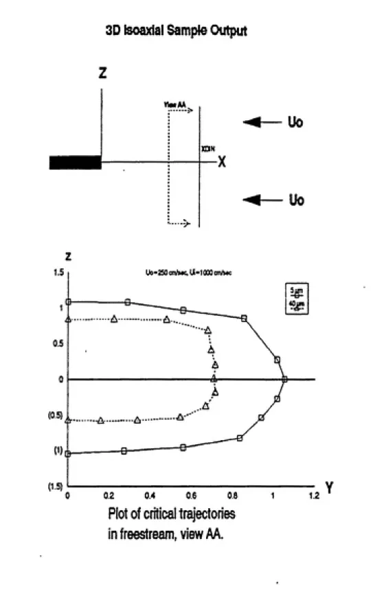
Figure 7 is an example of output for an isoaxial set of

conditions. The plot consists of the location of the

critical trajectories in the y-z plane at a constant value

of X (distance in front of the sampling inlet) equal to XDIN

in equation (24). In this case, x is constant because the

sampling angle is 0* and the freestream is flowing in a

direction perpendicular to the plane at x = XDIN.

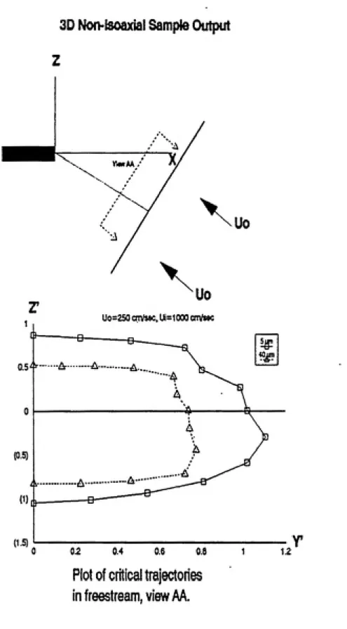
The plot in figure 8 represents the area in the

freestream, Ao, which is perpendicular to the freestream

resultant velocity for the case when the sampling angle was

30°. In this case, a simple plot of the y-z coordinates

would not represent the actual area of Ao as x was not

constant over the plane of interest. To solve this problem

the critical trajectory coordinates were converted to a

local coordinate system centered around the coordinates of

the initial capture point. First the distance, s, between

the first capture point and the critical trajectory

coordinate on each of the 13 rays defined by a, the

incremental angle, was calculated using the distance

formula, equation (22). After the distances between the

points were calculated, the x and y coordinates of the

critical trajectories determined using the following

Y' = s cosa (26)

Z' = s sina

RESULTS

Several combinations of free stream velocity, Uo, inlet

size, di, inlet sampling velocity, Ui, sampling pitch angle

(misalignment to the free stream), and particle aerodynamic

diameter, dae, were run through the 2D and 3D programs.

Table 1 summarizes the input variables which coincide with

input parameters used by Wiener (1987).

TABLE 1

Model Input Parameters

di Uo Ui dae theta

cm________cm/sec____cm/sec____micron degrees

.32 250 125 5.0 0

1.0 500 250 40.0 30

1000 500

1000

The two dimensional program was run for 96 combinations

of particle size (dae), velocity ratio (Uo/Ui), sampling

angle (6), and inlet diameter (di). The results are

summarized in the appendix.

A linear regression of the BIEM predicted aspiration

efficiency on the empirical aspiration efficiency calculated

from the unified aspiration model, equation (2), was

performed for all 2D data collected, for all 0"

combinations, and all 30° combinations. The results are

the 2D aspiration simulation versus the unified aspiration

model, equation (2).

TABLE 2

Two Dimensional Model Linear

Regression Results

CATEGORY SLOPE Y INT LCL(i) UCL!2) R2( 3)

All Data All 0° All 30° 0.842 0.963 0.664 0 0 0 074 077 118 0.788 0.941 0.599 0.895 0.986 0.729 0.917 0.993 0.911

(1) LCL - 95% lower confidence limit for slope

(2) UCL - 95% upper confidence limit for slope

(3) R2 - correlation coefficient

The 3D results are presented in the appendix and

summarized in figures 12, 13, and 14. Table 3 contains the

linear regression results which compare the numerical

prediction of aspiration efficiency with the unified model

of Hangal and Willeke, 1990.

TABLE 3

Three Dimensional Model Linear

Regression Results

CATEGORY SLOPE Y INT LCL <1) UCL12! R2 ( 3)

All Data All 0° All 30° 1.062 1.059 1.064 -0.062 -0.026 -0.096 1.026 1.036 0.980 1.099 1.082 1.148 0.995 0.999 0.991

(1) LCL - 95% lower confidence limit for slope

(2) UCL - 95% upper confidence limit for slope

Alt 2D (0 and 30 degrees)

2 4 6

Unified Model Aspiration Efficiency

Figure 9. 2D results, all data. Plot of the predicted

efficiency developed from the BIEH and Alenius theories

against the empirical unified aspiration efficiency model of

Isoaxial Case (0 degrees)

ct#

2 4 6

Unified Model Aspiration Efficiency

Figure 10. 2D results, isoaxial data. Plot of the

predicted efficiency developed from the BIEM and Alenius

theories againstthe empirical unified aspiration efficiency

Non-lsoaxiai Case (30 degrees)

4

J2^

2 4 6

Unified Model Aspiration Efficiency

Figure 11. 2D results, no'n-isoaxial data. Plot of the

predicted efficiency developed from the BIEM and Alenius

^6

-C

(D

O

IE

lu

c

0

%

a

(0

<

0)

All 3D (0 and 30 Degrees)

4

-D /^

u

^

X

2 4 6

Unified Model Aspiration Efficiency

Figure 12. 3D results, all data. Plot of the predicted

efficiency developed from the BIEM and Alenius theories

against the empirical unified aspiration efficiency model of

3D Isoaxlai Case (0 degrees)

LlMcfPirtiet

2 4 6

Unified Model Aspiration Eficiency

Figure 13. 3D results, isoaxial data. Plot of the

predicted efficiency developed from the BIEM and Alenius

theories against the empirical unified aspiration efficiency

3D Non-lsoaxlai Case (30 degrees)

LiMofPwfial

2 4 6

Unified Model Aspiration Efficiency

Figure 14. 3D results, non-isoaxial data. Plot of the

predicted efficiency developed from the BIEM and Alenius

theories against the empirical unified aspiration efficiency

DISCUSSION

The two dimensional model showed good agreement with

the unified aspiration model for the isoaxial conditions.

From table 2, the slope of the regression line for the 0"

sampling angle is 0.96. A slope of 1.0 would indicate

perfect agreement with the unified model. The largest error

in the 2d model occurred when the velocity ratio was less

than 1. In this case, the inlet velocity was 2 to 4 times

greater than the wind velocity leading to large changes in

air velocity and direction as the particles approached the

inlet face.

The nonisoaxial 2D model was tested for a 30° sampling

angle and showed poor agreement with the unified model. The

percent difference between the unified model aspiration

efficiency and the predicted aspiration efficiency was as

large as -71%. The slope of the regression line for this

set of conditions was .66.

Overall, the 2D model fairly represented the aspiration

efficiency of aerosols into a thin edged inlet. The

regression equation, slope of 0.84, was biased due to the

poor agreement of the 30° model with the unified model.

As shown in table 3, the three dimensional solution

performed significantly better in all categories when

compared to the 2D model. The slopes of the regression

lines were close to 1.0 for all cases indicating that the

values when compared to the unified aspiration efficiency

model. Table 4 shows a comparison of the 2D percent error

with that of the 3D model for the same combinations of

velocity ratios, sampling angle and particle diameter. As

can be seen, in most cases, the 3D model led to an

improvement in the aspiration efficiency value.

TABLE 4

Comparison of 2D Model Error

uo UI THETA DP 2D ERR 3D ERR

1000 125 0 5 22% 2%

1000 125 0 40 4% 5%

250 1000 0 5 12% -9%

250 1000 0 40 26% 9%

1000 125 30 40 -39% 5%

250 1000 30 5 -11% -11%

250 1000 30 40 -3% -10%

500 500 0 5 1% 3%

500 500 30 5 -10% 0%

500 250 0 5 _{11% 6%}

500 250 30 5 -6% 7%

500 125 0 5 26% 4%

500 125 30 5 17% 10%

Some error was introduced into the above comparison

because the unified model of aspiration efficiency was

developed for circular, thin edged inlets. This may have

some effect on the comparison of calculated efficiency with

the aspiration efficiency derived from the computer. This

does not, however, affect the model calculation of

efficiency because the actual areas using the square inlet

Boundary discretization, particle start point,

convergence criteria, and time step (f) were the most

important parameters in determining accurate solutions.

Boundary discretization had to be dense enough so that

calculations of internal velocities were performed at

distances greater than the distance between nodes on the

nearest boundary (Flynn and Miller, 1989). This was

accomplished by developing a 2D boundary consisting of 75

nodes with dense discretization near the inlet face and

along the inlet sides. The appendix contains a sample input

file for the 2D boundary discretization. With this

discretization, few aberrations in internal velocity

calculations were seen. This was not the case for the 3D

solution.

The three dimensional model boundary discretization

was proportional to the 2D discretization with the sides of

the triangular elements equal in length to the distance

between nodes in the 2D discretization. This led to an

input file containing 367 nodes defining 693 elements. As

described by Flynn and Miller, the triangular elements are

defined by numbering the element with the node numbers

corresponding to the vertices of the triangular element in a

clockwise fashion looking out of the domain. This was done

for approximately 1/2 of the elements starting at the inlet

face and along the walls of the inlet using a triangular

element generating program written for this problem. The

LOTUS spreadsheets because of the complex interactions of

common nodes along the edges of each facet of the cube and

at its corners.

Even with this dense 3D boundary discretization,

internal calculation of air velocities at points less than

0.05 cm from the face and walls of the inlet were extremely

inaccurate with the values being orders of magnitude larger

than the freestream velocity. This led to large errors in

the prediction of particle location which is dependent in

part on accurate calculation of air velocity at the

particle's current location. To avoid this error, capture

criteria for the particle was extended by a factor of 0.05

cm in front of the inlet face and around its edges. This in

effect enlarged the face area, Ai, to 1.11 cm^ for a square

inlet of side equal to 1.0 cm. This enlarged area was the

area used in the aspiration efficiency equation (18).

The effect of enlarging this area was to alter the

actual average air velocity moving into the "inlet". Over

the face of the inlet the air velocity was specified as Ui.

Over the thin layer defining the addition to the actual

inlet, the average velocity had a value which was a function

of the free stream velocity and the sampling velocity.

Because of this there is some error in the specification of

Ui in equation (184) and hence Ea.

Another problem with the 3D boundary discretization

velocity is also specified, but is different than that of

the first surface. In the final model, this occurred only

at the nodes surrounding the edges of the face of the

sampling inlet. Here, the velocity over the face was

specified as the sampling velocity, Ui, and the velocity on

the edge of the tube and along its length was specified as 0

cm/sec. This caused a discontinuity of velocity at the

edges of the sampling inlet. The effect of the

discontinuity was to cause inaccuracies in interpolation of

velocities over the elements involved. This interpolation

error was minimized by inserting a very thin row of elements

just inside the edges of the inlet. For the final model the

width of this small layer was 0.001 cm.

Particle start points were important because the

aspiration efficiency calculation requires the critical

trajectory start points to be in the free stream. It was

found that at distances of 6 inlet diameters from the inlet,

local air velocity and direction was within 5% of the

specified free stream velocity. This agrees with the

findings of Belyaev and Levin (1972) and held true for both

When determining the location of critical trajectories,

the distance between the last capture trajectory start point

and last miss trajectory start point was compared to the

convergence criteria. Once the distance reached a preset

the 2D model was set at 0.01 cm after iterations at criteria

smaller than this caused a less than 1% change in the

calculated efficiency. The convergence criteria for the 3D

model led to good agreement with the unified model when set

at 0.05 cm.

The time step was the most critical factor in

developing accurate particle trajectories. Time steps that

were too large resulted in predictions of trajectories that

were too coarse to accurately predict the particle movement.

Unnecessarily small time steps caused excessive computing

time. Through a series of program tests, 0.0003 seconds was

chosen as the time step for the 2D model with a further

reduction by a factor of 10 once the particle came within 1

inlet diameter of the sampling inlet to account for the

large velocity changes near the face of the inlet.

The time step and the convergence criteria for the 3D

model were not as sensitive in the determination of the

aspiration efficiency as they were in the 2D case. Since

the 3D model more realistically represented the physics of

the problem, accurate solutions were obtained for time steps

ranging from 0.001 to 0.0003 seconds with the time step

being halved when the particle was within 1 inlet diameter

of the inlet face.

Because the size of the time step indirectly predicts

the distance the particle will move; positions predicted

when the air is turning and accelerating will not lie on the

for velocity ratios of 2 and 4 where the estimate of Ea was

consistently larger than the unified model prediction. In

this case, the air is approaching the inlet faster than the

inlet is sampling and must diverge around the inlet.

Particle trajectories will also diverge but the predicted

position will lie slightly inside of the actual trajectory.

This causes an overestimate of Ao leading to an increase in

the prediction of Ea.

When running the model under certain conditions, the

time step and capture criteria became very critical in

determining whether a trajectory resulted in a miss or

capture. In the three dimensional model, when Uo = 1000, Ui

= 125 cm/sec, and 9 = 30°, the best estimate of aspiration

efficiency was off by 39% when compared to the unified

model. Under these conditions the air flow is approaching

the inlet at 8 times the sampling rate causing significant

divergence of the air streamlines around the face of the

inlet. This situation combined with the sampling angle

results in particle trajectories which move virtually

straight up in the positive z direction at locations within

0.1 cm of the inlet face when the particle is approaching

the inlet from above the centerline. The air velocity in

this area is also moving very fast. The combination of high

velocity particle and steep angle of approach toward the

situation when in actuality a capture should have occurred.

This causes an underestimation of Ao leading to a prediction

of Ea which is too small. This situation occurred for the

last four rays around the start point semicircle and is the

reason for the poor performance of the model under these

conditions. This situation can be eliminated by reducing

the size of the time step but would lead to a large increase

in computing. The same problem was seen in the 2D model and

prevented identification of an upper critical trajectory.

By specifiying an incremental angle of 15° in the 3D

model, the program was limited to locating 13 critical

trajectories. The effect of decreasing a has not been

analyzed but would lead to a finer outline of the critical

trajectory stream tube and a more accurate calculation of

Ao. One anomaly in the output was seen when the ray

specified conincided with the corners of the inlet.

Critical trajectories associated with these rays tended to

lie outside range of critical trajectories on either side of

this point. In one program test, eliminating these rays

from the program improved the model result from a 26% to a

4% error.

The results presented in this paper show that the

solutions agree with the unified empirical model of Hangal

and Willeke (1990). The advantage of this model is that it

can be expanded to situations beyond that investigated.

These situations include modeling a yaw angle, multiple

angle as opposed to a pitch angle would require only a shift

in the direction of the gravity component in the currently

available boundary file. Modeling of multiple inlets and

differing inlet geometries could be accomplished by

reworking boundary files to represent the new inlet

CONCLUSION

The boundary integral equation method can be used to

accurately describe the air flow field into a thin edged

inlet. Once the flow is described, Alenius's (1989)

analytical solution to the particle equations of motion can

be used to locate critical aerosol trajectories and

accurately predict aspiration efficiency, A simple two

dimensional model described here can accurately predict

aspiration efficiency for small particles when the velocity

ratio is close to 1. In this case, the critical

trajectories are symmetric about the center of the inlet.

When an angle of misalignment is introduced and/or the

velocity ratios differ significantly from 1.0, a three

dimensional model is required to describe critical

trajectories and thus aspiration efficiency.

The 3D model can accurately predict aspiration

efficiencies which are in good agreement with the unified

aspiration efficiency model for all forward sampling angles

proposed by Hangal and Willeke (1990). Further refinements

to the model should improve the accuracy of aspiration

efficiency estimates.

Finally, this model has the capability of predicting

aspiration efficiencies for inlets of differing shapes and

orientations including multiple inlets, yaw angles, and

inlets of differing geometry. By reworking the boundary

input files, inlets of any geometry, location, sampling

FUTURE WORK

Successful calculation of particle trajectories depends

on several adjustable variables in the program including

boundary discretization, calculation time step, convergence

criteria, and capture criteria. While this paper

demonstrates that the method can accurately track particles

for given conditions, the above variable have not been

tested to determine their optimum values. A study of these

variables will help determine the contribution of each to

the overall error in the program.

Boundary discretization of the 3D domain required to

solve the BIEM problem can be difficult due to the number of

triangular elements required. Also, when constructing a

closed domain, a number of common nodes appear along the

edges of each face of the boundary and at the corners. This

can lead to cases where one node is contained in up to 6

distinct triangular elements. Boundary files for this

project were manually prepared for about 50% of the domain.

Full automation of this process would greatly increase the

applicability of this method.

Finer discretization at the face of the inlet and along

the walls of the inlet will decrease the distance a particle

can come within the inlet and inlet sides before internal

air velocity calculations no longer represent the

conditions. In this project, that distance was 0.05 cm.

nodes and triangular elements required to describe the

boundary and may increase the size of the boundary file by

as much as 50% and subsequently increase computing time.

Finer discretization may be avoided by adding an

interpolation scheme to the program. This subroutine would

be invoked when the particle entered the volume around the

face of the inlet where internal velocity calculations

showed large error. While this will cause some error in the

prediction of internal velocity, it is expected it will be

less than that of assuming a captured trajectory has

occurred when the particle enters this area.

Rediscretization of the inlet and walls to more closely

represent a circular inlet may also lead to a better

comparison of the model with the unified aspiration

efficiency equation. This could be done by modelling the

inlet as an equal area hexagon or octagon. Automation of

the boundary file would be paramount in this case as the

discretization would become extremely tedious.

It may be necessary to add a routine to the program to

automatically decrease the time step if the distance between

successive points becomes large or the particle jumps across

the boundaries of the inlet. Alternatively, the path of the

particle can be analyzed to see if it crossed the inlet and

a routine added to the capture criteria which records a

capture when this situation occurs.

The boundary input files and start point routines were

not general enough to support negative (downward pointing)

inlet orientations. However, by simply changing the sign on

the gravity vector and representing the negative angle as a

positive angle, predictions of aspiration efficiency may be

obtained.

Combination of the 3D boundary solution program with

the particle tracking routine and the area integration

routine would further streamline the efficiency

Calculation of Particle Trajectories:

Particle transport is influenced by a gravity force and

a drag force due to the friction of the surrounding air. By

Newton's second law, particle mass times acceleration is

equal to the sum of the forces on the particle,

€

F = ma (1)

where F is the force, a is the acceleration and bold face

quantities represent vectors.

The frictional force can be expressed by the following

equation:

Fd = - Cd(Re) Ap pi vr vr (2)

CC 2

where

Cd(Re) is the dimensionless friction factor

dependent on the Reynolds number

CC is the Cunningham slip correction

Ap is the projected area of the particle

pi is the density of the medium (air)

vr is the particle velocity relative to the

Cd(Re) is dependent on the particle Reynold's number,

Re = vr dp pi (3)

Ml

where

dp is the particle diameter (assumed

spherical)

fjl is the viscosity of the air.

Several expressions for Cd(Re) can be found in the

literature (Reist, 1984) with most yielding no major

deviation (Alenius, 1987). For this project the expressions

used by Alenius are incorporated into a simplifying

expression:

Cd(Re)=24/Re Q(Re)

where Q(Re) is defined as: (4)

Q(Re) = 1 for 0 < Re <= 0.5

Q(Re) = 1 + 0.15 Reo-6e7 for 0.5 < Re <= 800

Q(Re) = 0.44 Re/24 for 800 < Re < 20000.

By combining equations (3) and (4) into equation (2)

and Introducing the expression for particle relaxation time,

Fd/m = Q(Re)/T vr (5)

where

T = dp» pi CC (6)

18 Ml

From equations (1) and (5) the particle motion can be

described as:

d2r/dt2 - [Q(Re)/T(u-(dr/dt))]-g = 0 (7)

where

r is the particle position vector

g is the acceleration due to gravity

u is the air velocity at the point where

the particle is located.

Equation (7) is analytically solvable if the factor

Q(Re) is constant and the air velocity u at the points where

the particle is successively located can be described as a

linear function of the time that has elapsed until the

particle reached the point. This condition can be

approximately met it the motion is calculated in

sufficiently small time steps.

If we introduce an expression for the linear behavior

of the air velocity over the time interval being studied,

u(t) = (u(t)-u(t-t')/t'+b (8)

where

t is time

t' is the length of the time step

b is some initial value of velocity

For ease of writing we define the first part of the above

expression as ua:

ua = (u(t)-u(t-f)/f) (9)

Now if we let A=Q(Re)/T equation (7) can be rewritten

as:

dv/dt - A(uat+b) + Av - g = 0

recognizing that d^r/dt^ = dv/dt,

or, dv/dt + Av = A(uat+b)- g (10)

If equation (10) is multiplied through by e*t the left

hand side of the equation will be a derivative.

eAt(dv/dt) + e*t(Av) =(eAt)A(uat+b)- g(eAt)

Integrating both sides of the above equation from tl to t2

gives:

v,t2)eAt2-V(ti)e*ti = [(uat2)e*t2 - (ua/A)eAt2

+(b)eAt2 + (g/A)eAt2]

- [(uat2)e*ti - (ua/A)eAti

58

Adding V(ti)e*'^i to both side of the equation, dividing

through by 0**2 and simplifying gives an expression for

V(t2):

v<t2) = uat2 - ua/A + b + g/A

- {(uatl) - ua/A + b + g/A - V(11>}eA(11 -12> (12)

If we define a simplifying term,

Ub = u(t)-(Ua-g)T/Q(Re)

and define tl as t, and t2 as the time at the end of the

times step, t' (t2 = t + t'), substitute the air velocity at

time t for b, and replace A with Q(Re)/T, then the solution

is:

v(t+f) = Uat'+Ub-(Ub-v(t))exp-tQ(Re)t'/T] (13)

Integrating the equation (13) again will give the particle

position:

r(t+t') = r(t)+Ua/2f2+Ubt'

-(Ub-v(t))T/Q(Re)(l-expQ(Re)f/T) (14)

Equation (13) and (14) are analytical solutions to the

particle equations of motion and are used in both the 2D and

2D Boiindary Discretization Sample:

Potential specified on top and rear sides.

Velocity specified over front, bottom, inlet face

and sides.

DIN 1 cm

THETA 30

_degrees

cm/sec

UO -250

_cm/sec

UOY 125

(inlet diameter)

(nozzle angle)

(sampling velocity)

(wind velocity)

(x component of UO)

(y component)

NODE PHI DPHI ID ICT

1 20 2 20 3 20 4 20 5 20 6 20 7 20 8 20 9 19.99 10 15 11 10 12 5 13 0 14 -5 15 -10 16 -15 17 -20 18 -20 19 -20 20 -20 21 -20 22 -17.5 23 -15 24 -12.5 25 -10 26 -7.5 27 -5 28 -4.5 29 -4 30 -3.5 31 -3 32 -2.5 33 -2 34 -1.5 35 -1

15 0 -216 .5064 3 0

10 0 -216 5064 3 0

5 0 -216 .5064 3 0

0 0 -216 5064 3 0

-5 0 -216 .5064 3 0

-10 0 -216 5064 3 0

-15 0 -216 5064 3 0

-20 0 -216 5064 3 0

-20 0 -125 3 0

-20 0 -125 3 0

-20 0 -125 3 0

-20 0 -125 3 0

-20 0 -125 3 0

-20 0 -125 3 0

-20 0 -125 3 0

-20 0 -125 3 0

-20 1830 13 0 2 1

-15 2455. 13 0 2 0

-10 3080 13 0 2 0

-5 3705. 13 0 2 0

-0.5 4267 .63 0 2 2

-0.5 0 0 3 0

-0.5 0 0 3 0

-0.5 0 0 3 0

-0.5 0 0 3 0

-0.5 0 0 3 0

-0.5 0 0 3 0

-0.5 0 0 3 0

-0.5 0 0 3 0

-0.5 0 0 3 0

-0.5 0 0 3 0

-0.5 0 0 3 0

-0.5 0 0 3 0

-0.5 0 0 3 0

51 -2 0.5

52 -2.5 0.5

53 -3 0.5

54 -3.5 0.5

55 -4 0.5

56 -4.5 0.5

57 -5 0.5

58 -7.5 0.5

59 -10 0.5

60 -12.5 0.5

•

61 -15 0.5

62 -17.5 0.5

63 -20 0.5

64 -20 5

65 -20 10

66 -20 15

67 -20 20

68 -15 20

69 -10 20

70 -5 20

71 0 20

72 5 20

73 10 20

74 15 20

75 20 20

•

0 3 0

0 3 0

1000 3 0

1000 3 0

1000 3 0

1000 3 0

1000 3 0

1000 3 0

1000 3 0

1000 3 0

1000 3 0

0 3 0

0 3 0

0 3 0

0 3 0

0 3 0

0 3 0

0 3 0

0 3 0

0 3 0

0 3 0

0 3 0

0 3 0

0 3 0

0 3 0

0 3 0

0 3 0

0 2 1

0 2 0

0 2 0

0 2 0

0 2 0

0 2 0

0 2 0

0 2 0

0 2 0

0 2 0

0 2 0

0 2 0

216.5064 3 2

3D Boundary Discretization Sample;

INPUT FILE FOR 3D CASE, 367 NODE, 693 ELEMENTS

Potential specified at all faces except at boudary of tube

and at the face. I>ur corners specified with potential.

DIN 1 cm (inlet diameter)

THETA 30 degrees (nozzle angle)

UI 1000 cm/sec (sampling velocity)

UO -250 cm/sec (wind velocity)

UOX -216.5064 (x component of UO)

UOY 0 (y component)

NODE X Y 2 PHI DPMI ID ICT

1 0 -0.5 -0.5 0 0 2 0

2 0 -0.5 -0.499 0 0 2 0

3 0 -0.5 -0.375 0 0 2 0

4 0 -0.5 -0.25 0 0 2 0

5 0 -0.5 -0.125 0 0 2 0

6 0 -0.5 0 0 0 2 0

7 0 -0.5 0.125 0 0 2 0

8 0 -0.5 0.25 0 0 2 0

9 0 -0.5 0.375 0 0 2 0

10 0 -0.5 0.499 0 0 2 0

11 0 -0-5 0.5 0 0 2 0

12 0 -0.499 -0.5 0 0 2 0

13 0 -0.499 -0.499 0 1000 2 0

14 0 -0.499 -0.375 0 1000 2 0

15 0 -0.499 -0.25 0 1000 2 0

16 0 -0.499 -0.125 0 1000 2 0

17 0 -0.499 0 0 1000 2 0

18 0 -0.499 0.125 0 1000 2 0

19 0 -0.499 0.25 0 1000 2 0

20 0 -0.499 0.375 0 1000 2 0

21 0 -0.499 0.499 0 1000 2 0

22 0 -0.499 0.5 0 0 2 0

23 0 -0.375 -0.5 0 0 2 0

24 0 -0.375 -0.499 0 1000 2 0

25 0 -0.375 -0.375 0 1000 2 0

26 0 -0.375 -0.25 0 1000 2 0

27 0 -0.375 -0.125 0 1000 2 0

28 0 -0.375 0 • 0 1000 2 0

29 0 -0.375 0.125 0 1000 2 0

30 0 -0.375 0.25 0 1000 2 0

31 0 -0.375 0.375 0 1000 2 0

32 0 -0.375 0.499 0 1000 2 0

33 0 -0.375 0.5 0 0 2 0

34 0 -0.25 -0.5 0 0 2 0

35 0 -0.25 -0.499 0 1000 2 0

36 0 -0.25 -0.375 0 1000 2 0

37 0 -0.25 -0.25 0 1000 2 0

38 0 -0.25 -0.125 0 1000 2 0

39 0 -0.25 0 0 1000 2 0

40 0 -0.25 0.125 0 1000 2 0

41 0 -0.25 0.25 0 1000 2 0

42 0 -0.25 0.375 0 1000 2 0"

43 0 -0.25 0.499 0 1000 2 0

44 0 -0.25 0.5 0 0 2 0

45 0 -0.125 -0.5 0 0 2 0

46 0 -0.125 -0.499 0 1000 2 0

47 0 -0.125 -0.375 0 1000 2 0

48 0 -0.125 -0.25 0 1000 2 0

49 0 -0.125 -0.125 0 1000 2 0

50 0 -0.125 0 0 1000 2 0

51 0 -0.125 0.125 0 1000 2 0

52 0 -0.125 0.25 0 1000 2 0