A Proactive Context-Aware Self-Healing
Scheme for 5G Using Machine Learning
Shirin Nikmanesh
Department of Technology and Engineering Central Tehran Branch, Islamic Azad University
Tehran, Iran
Mohammad Akbari
Communication Technology Faculty ICT Research Institute (ITRC)
Tehran, Iran [email protected]
Roghayeh Joda*
Communication Technology Faculty ICT Research Institute (ITRC)
Tehran, Iran [email protected]
Received: 7 May 2018 - Accepted: 3 September 2018
Abstract—Future mobile communication networks particularly 5G networks require to be efficient, reliable and agile to fulfill the targeted performance requirements. All layers of the network management need to be more intelligent due to the density and complexity anticipated for 5G networks. In this regard, one of the enabling technologies to manage the future mobile communication networks is Self-Organizing Network (SON). Three common types of SON are self-configuration, Self-Healing (SH) and self-optimization. In this paper, a framework is developed to analyze proactive SH by investigating the effect of recovery actions executed in sub-health states. Our proposed framework considers both detection and compensation processes. Learning method is employed to classify the system into several sub-health (faulty) states in detection process. The system is modeled by Markov Decision Process (MDP) in compensation process in which the equivalent Linear Programing (LP) approach is utilized to find the action or policy that maximizes a given performance metric. Numerical results obtained in several scenarios with different goals demonstrate that the optimized proposed algorithm in compensation process outperforms the algorithm with randomly selected actions.
Keywords-component; fifth generation cellular network (5G), self-organizing networks (SON), self-healing, fault detection and compensation, markov decision problem (MDP), linear programming, machine learning, K-means clustering
I. INTRODUCTION*
Exponential increase in connected devices and variety of services with the diverse requirements in 5G networks involve the network management systems
* Corresponding Author
with new challenges in order to satisfy the user expected quality of service (QoS) and quality of experience (QoE) [1]. Obviously, the above challenges will be more critical when new technologies such as network slicing [2] and mobile edge computing (MEC)
are utilized [3]. This problem demands management and operation of the network to be more autonomous smart and agile. One of the well-known concepts in agile and intelligent management of the network is SON where is discussing in the literature in the past couple of years. Hence, by employing SON in the
mobile communication networks, network
management will be more smart, automated and adaptive while human intervention will be minimized [4].
3GPP standardization from releases 8 to 14 categories different issues of SON into three major types, i.e., Configuration, Healing and Self-Optimization [4]. SON operating in several areas such as multi Radio Access Technology (multi-RAT) networks, Management and Orchestration (MANO), vertical industries and network slices are set in managing of 5G networks [5]. Healing process which is the focus of this paper contains monitoring the performance, detecting faults and failures, activating compensation and recovery phases and finally analyzing the results. In fact, healing improves the network reliability and simultaneously decreases the cost of operation [6].
Recently, meaningful efforts and researches have been done on SON as a very beneficial solution in increasing the performance of the network and users’ quality of experience and at the same time in decreasing the costs related to management and operation of the network. However, several challenges that make current SON algorithms to be inappropriate for 5G communication networks. Thus, [8] proposes a comprehensive framework to enrich SON algorithms with available big data. In fact, there is currently a huge amount of data in mobile networks and it will be much more in future dense 5G networks that causes the SON algorithms to be very complicated [9].
Current state-of-the-art solutions are moving toward more intelligence SON algorithms for mobile communication networks. The new algorithms that are being developed, take advantage of complex but effective ML algorithms [10]. In [11], the authors deal with automatic detection of sleeping cell (SC) in the network as a way for decreasing maintenance cost and enhancing network performance. The SC is defined as a cell which does not provide expected services to the users. The purpose of [11] is to optimize network efficiency while lowering maintenance and operational cost. To this purpose, an intelligent ML framework is presented that utilizes minimize drive testing (MDT) to collect key PIs (KPI’s) of a LTE network. Employing context information for automatic failure management in small-cell indoor scenarios is proposed by [12]. This paper identifies the user equipment (UE) as the major source of information and proposes a framework for integrating context awareness and SH. Furthermore, detailed context-based detection and diagnosis mechanisms are developed.
In [13], K-means algorithm is applied on the evidences extracted from the suspicious nodes. This automatic clustering algorithm provides better prediction for the files need to be assessed more into depth. These files are called outliers. The remaining
files assumed to be normal. The number of clusters is considered unknown in general.
Hence, a method is proposed for determining the number of clusters from the observations. The proposed method is the Elbo method. The K-means clustering technique is also used in [14] to process MDT measurements in order to detect efficiently a sleeping cell. For a comprehensive review of the proposed ML-based techniques in SH process in mobile communication networks refer to [15].
SON address the radio access network (RAN) and the core of the mobile communication network. A new algorithm is presented in [16] to detect and solve problems related to the radio interface by considering both mobile traces and SON. The proposed method precisely locate RF problems according to the evaluation of the RF conditions. Utilizing the performance indicators (PIs) and employing a supervised technique, [17] proposes a Self-Healing algorithm in which the dissimilarity of the behavior of the network statistics in various network states is employed.
SON agents need to operate jointly for avoiding the confliction. This issue is considered in [18] by applying Rosen's concave games for the cooperation between different SON agents. Discovering the degraded cells using the time evolution of several metrics is addressed in [19] in which the faulty pattern of the cell is compared with a set of fictitious degraded patterns.
SH can be realized in two reactive and proactive manners depending on whether it would trigger just when a problem has already occurred or it is based on predicting and preventing that problem in advance [20]. The reactive-SH functionality already implemented in 3G/4G is not able to meet 5G performance requirements (e.g., the zero latency perception requirement) and the targeted QoE levels [10]. Therefore, a challenging-transition from reactive to proactive scenarios is necessary in 5G context. Proactive SH is used in [10] by collecting the data and creating proper models. Several techniques can be used according to the available data that feeds the model. From learning aspects view point, [10] surveys SON algorithms and solutions.
The reliability behavior of a base station is modeled by Continuous Time Markov Chain (CTMC). Moreover, [21] presents a framework to predict the faults by employing the developed model and subsequent analysis in which the sub-health state is considered between optimal operation and outage states. However, it does not investigate the impact of actions executed in sub-health states.
In this paper, we develop a scheme to implement a proactive SH process including detection and compensation processes in an extended healing model considering sub-health states. Thus, the operator can opt the actions or policies so that maximizes the long term rewards. To this end, our system is considered as a Markov Decision Process (MDP) which is a fundamental formulation for stochastic decision making.
In MDP, we have a set of states and actions accomplished in each state to control the behavior of the system so as to maximize a given performance metric [22]. Detection and compensation processes require the number of sub-health states and therefore, we apply K-means clustering technique to figure out the number of these states.
The rest of the paper is organized as follows. Section II presents the system model in two main parts: A. fault detection and model's parameters extraction and B. compensation process. In Section III, the analysis of the proposed scheme is described for compensation process and determining the optimal policy. The numerical results are given in Section IV and the conclusions are finally provided in Section V.
II. SYSTEM MODEL
The general block diagram of the system model is depicted in Fig. 1. The detection and compensation processes both are included in the model. Measured data from the network is processed by detection block to distinguish faulty states. The proposed method is to classify system states into faulty, outage and normal states of the operation utilizing the k-means algorithm, which is a machine learning (ML) technique belongs to the category of unsupervised learning. A set of unlabeled input data denoted as a training set will be used to correctly learn the faulty states. The utilized data set for this purpose is derived from [23] which is a collection of standard and prevalent key performance indicators (KPI) given in Table I.
TABLE I. KEY PERFORMANCE INDICATORS USED IN DETECTION PROCESS [23]
KPI
Measurements KPI Description
Retainability
The number of successfully finished connections to the total number of successfully-initiated connections ratio HOSR Handover success rate RSRP Reference signal received power RSRQ Reference signal received quality SINR Signal to interference & noise ratio
Throughput Maximum data rate is transferred through a system
Based on this context information, KPI statistics, a detection algorithm is proposed to detect the faulty states utilizing K-means clustering algorithm.
The learned clusters employing training data is used for classifying the ongoing observations into faulty, outage and normal state. As stated, the proposed method for detection includes determining the current sub-health state that the system belongs to.
In order to determine the optimal action that should be executed to recover the system into normal operation at the next step, the proposed model is adapted to decision making formalism in stochastic domains adopting Markov Decision Process (MDP).
MDP is a system comprising a set of some intuitive states and actions. These actions can be carried out in a way to maximize some desired performance criterion [22].
A. Fault Detection and Model's Parameters Extraction
The 𝐾-Means clustering is a powerful and popular unsupervised clustering algorithm for clustering and determining the centroid points of the clusters among a set of unlabeled data [13]. The algorithm just requires two parameters for initializing: a) the training data set and b) the desired number of clusters indicated by 𝐾.
Based on minimum distance of each data to the centroid point of the 𝐾 clusters (which is determined iteratively through the algorithm), K-Means partitions data into 𝐾 distinct clusters. The time complexity of this algorithm is 𝑂(𝑅, 𝐾, 𝑛) [13], where, 𝑛 is the number of input data, 𝐾 is the number of clusters and 𝑅 is the number of repetitions to convergence. Typically, both 𝐾 and 𝑡 parameters have small values which makes the 𝐾-means an efficient linear algorithm. This algorithm is elaborated in Algorithm 1 [10]. An important challenge is to determine K, the number of clusters. The utilized method in this paper for determining K is elbow method [13]. This method helps to select the optimal number of clusters K by fitting the model with a range of test values for K. In a curve that demonstrates ‘within-cluster sum of squared errors (SSE)’ against ‘the candidate values for K’, the elbow point is defined as the point of inflection on the curve. Here, the error is the distance of each data sample to its centroid point. The corresponding K of elbow point is the best candidate for the number of clusters in underlying model.
Model's Parameters Extraction: - Number of clusters k - MDP parameters
Training Data set
Observed KPIs
K-means Classifier
Detection Process
MDP
Select Optimum Action for Recovery
Optimum Policy
Compensation Process
Figure 1. System model block diagram
Algorithm1 : K-means Algorithm
Input: Initial Data set (D), desired number of clusters (𝐾)
1: initialize 𝑲 cluster centroids from data points selected randomly (seeds),
2: while not converged do
3: for each centroid, identify the closest data points
4: Compute means using the current cluster memberships and reassign new centroids
5:end while
B. Compensation Process
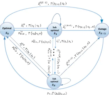
Quantitative MDP model is considered to determine the optimal actions which can be executed by the operator. The model is depicted in Fig. 2. The number of clusters denoted by 𝐾 corresponds to the number of sub-health states in the MDP model. In SH process, the decision making is fulfilled by a centralized module called SH-agent. Hence, the decision making process is modeled as a quantitative MDP as shown in Fig. 2.
In MDP context, there are two intuitive set of states and actions. In order to maximize some desired performance criteria, the actions accomplish so that control the environment's state properly. . The MDP model is recognized by the distinctive characteristic of being memory less in which the chosen action at each state is independent of previous actions. In the circumstances of this paper, the proposed MDP model of Fig. 2 is fully characterized by a set of 4 distinctive quantities. These quantities are states, actions, transitions rate between states and a reward function that are expressed as (𝓢, 𝓐, 𝑇, 𝑟)respectively. In the context of mobile cellular networks and SON, the Markov models are popular and mainly applied to analyze self-optimization (SO) and SH [10].
We assume that the time is divided into time slots with specific duration of 𝑇. Therfore, a discrete-time MDP (DT-MDP) model is considered. . Thus, in order to discuss the time-dependent variables such as states, we define variable 𝑡 = 1, 2, … representing the consecutive time instants. . Let 𝑠(𝑡) ∈ 𝓢 = {𝑠0, 𝑠1, … , 𝑠𝑁, 𝑠𝑁+1}denotes the system state at time
instant 𝑡, where 𝑠(𝑡) = 𝑠0 and 𝑠(𝑡) = 𝑠𝑁+1 represent
optimal and outage states respectively. The other states {𝑠𝑖}𝑖=1𝑁 represent the sub-health (or sub-health) stats. In
sub-health stats the desired performance indicators (PIs) deviate from their optimal values but it is assumed that the outage has not occurred yet. Where it wouldn’t lead to ambiguity, for seeking simplicity we might ignore 𝑡 occasionally..
In a sub-health state, the system can continues to operate while the KPIs degrade below the desired level [21]. It is noteworthy that the sub-health states {𝑠𝑖}𝑖=1𝑁
sorted in deteriorating manner. As a result, 𝑠1 and 𝑠𝑁
represent best and worst sub-health states respectively. The model implies that for each possible fault/failure case, a specific model with different parameters should be considered. Similar to [21], in the proposed model, failures are categorized into two distinct categories. The first one is trivial failures. A trivial failure does not cause full outage but drive the state from optimal state 𝑠0 to one of the sub-health states {𝑠𝑖}𝑖=1𝑁 . On the other
hand, critical failures are considered in which drive the system to full outage 𝑠𝑁+1. The later occurs in optimal
or one of the sub-health states. The failures are assumed to be temporarily independent. The arrival rate of 𝜆𝑡𝑖𝑗 and 𝜆𝑐𝑖𝑗 are trivial and critical failures from states 𝑖 to 𝑗 respectively (Fig.2) and can be modeled using Poisson distribution.
When misbehavior detected, normally at the sub-health or outage states, an error/failure recovery module will activated. ,. Let finite set 𝓐 = {𝑎1, 𝑎2, … , 𝑎𝐴} with
size |𝓐| = 𝐴 be the set of all possible actions at each state 𝑠 ∈ 𝓢. We keep the generality of formulation here by considering probabilistic policies. Defining 𝜋(𝑎|𝑠) as the probability of choosing action 𝑎 in state 𝑠,
Optimal Sub Outage
optimal
Sub optimal
Figure 2. MDP-based decision making process
according to an optimal policy 𝜋(𝑎|𝑠), the recovery module selects action 𝑎 ∈ 𝓐 and tries to get the system back to optimal state from sub-health state 𝑠.
Taking action 𝑎, the time duration which takes the system to moves from sub-health state 𝑠𝑖 to state 𝑠𝑗
(sub-health or optimal) is assumed to be exponentially distributed. This time includes the required time for anomaly detection, diagnosis and compensation with mean value of 1/𝜇𝑑𝑐,𝑎𝑖𝑗 (or 1/𝜇𝑑𝑐,𝑎𝑖0 ) [21]. The
compensation time required for retrieving outage to optimal state is also assumed to be exponential with mean value 1/𝜇𝑐.
Let 𝑇(𝑠′|𝑠, 𝑎) be the probability of transition from
state 𝑠 to a new state 𝑠′ ∈ 𝑺 accomplishing action 𝑎 ∈ 𝓐. Then, the transition matrix 𝑻 will be as follow:
𝑻 =
[
𝑇(𝑠0|𝑠0) 𝑇(𝑠0|𝑠1, 𝑎1) 𝑇(𝑠1|𝑠0) 𝑇(𝑠1|𝑠1, 𝑎1) ⋯
𝑇(𝑠0|𝑠𝑁, 𝑎𝑁) 𝑇(𝑠0|𝑠𝑁+1) 𝑇(𝑠1|𝑠𝑁, 𝑎𝑁) 𝑇(𝑠1|𝑠𝑁+1)
⋮ ⋱ ⋮
𝑇(𝑠𝑁|𝑠0) 𝑇(𝑠𝑁|𝑠1, 𝑎1) 𝑇(𝑠𝑁+1|𝑠0) 𝑇(𝑠𝑁+1|𝑠1, 𝑎1) …
𝑇(𝑠𝑁|𝑠𝑁, 𝑎𝑁) 𝑇(𝑠𝑁|𝑠𝑁+1) 𝑇(𝑠𝑁+1|𝑠𝑁, 𝑎𝑁) 𝑇(𝑠𝑁+1|𝑠𝑁+1)]
,
(1) where, 0 ≤ 𝑇(𝑠′|𝑠, 𝑎) ≤ 1, ∀ 𝑠, 𝑠′∈ 𝓢 & ∀𝑎 ∈ 𝓐 represents the probability of going to state 𝑠′ accomplishing action 𝑎, when the system is in state 𝑠. According to Fig. 2 and as evidence in (1), we only do action in sub-health states {𝑠𝑖}𝑖=1𝑁 . In the other words,
recovery action in outage sate 𝑠𝑁+1 is not included in
proactive MDP model.
Considering reward 𝑟 (𝑠′|𝑠, 𝑎), ∀(𝑠′, 𝑠) ∈
𝓢 & 𝑎 ∈ 𝓐 for particular transitions to 𝑠′ from 𝑠
accomplishing 𝑎, the reward matrix 𝑹 is denoted by:
𝑹 =
[
𝑟(𝑠0|𝑠0) 𝑟(𝑠0|𝑠1, 𝑎1) 𝑟(𝑠1|𝑠0) 𝑟(𝑠1|𝑠1, 𝑎1) ⋯
𝑟(𝑠0|𝑠𝑁, 𝑎𝑁) 𝑟(𝑠0|𝑠𝑁+1) 𝑟(𝑠1|𝑠𝑁, 𝑎𝑁) 𝑟(𝑠1|𝑠𝑁+1)
⋮ ⋱ ⋮
𝑟(𝑠𝑁|𝑠0) 𝑟(𝑠𝑁|𝑠1, 𝑎1) 𝑟(𝑠𝑁+1|𝑠0) 𝑟(𝑠𝑁+1|𝑠1, 𝑎1) …
𝑟(𝑠𝑁|𝑠𝑁, 𝑎𝑁) 𝑟(𝑠𝑁|𝑠𝑁+1) 𝑟(𝑠𝑁+1|𝑠𝑁, 𝑎𝑁) 𝑟(𝑠𝑁+1|𝑠𝑁+1)]
.
(2) Generally, our most important goal is determining the optimal policy 𝜋(𝑎|𝑠) which maximizes the expected reward in long term with adopting that policy in a pretty long sequence of decision making and doing actions. The MDP push decisions toward achieving maximum non-zero rewards. Consequently, the strategy in assigning the rewards 𝑟 (𝑠′|𝑠, 𝑎) determines
the aim of MDP. The aforementioned variables and parameters are summarized in Table II.
The described model above is an analytical model can be adopted to model a typical proactive healing process. This SH process could deal with any generic faults or failure cases that may happen in hardware or software. Considering a predefined goal, in section III, we will develop an analytically tractable MDP to model our decision making in SH process. The purpose of this modeling is to analyzing the decision making process and determining the optimal policy 𝜋(𝑎|𝑠).
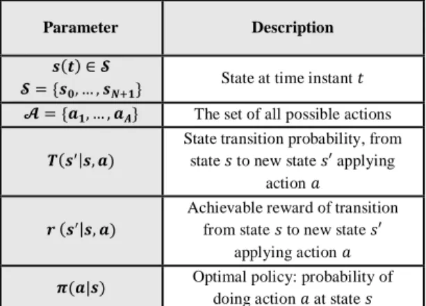
TABLE II. MDP MODEL PARAMETERS
Parameter Description
𝒔(𝒕) ∈ 𝓢
𝓢 = {𝒔𝟎, … , 𝒔𝑵+𝟏} State at time instant 𝑡 𝓐 = {𝒂𝟏, … , 𝒂𝑨} The set of all possible actions
𝑻(𝒔′|𝒔, 𝒂)
State transition probability, from state 𝑠 to new state 𝑠′ applying
action 𝑎
𝒓 (𝒔′|𝒔, 𝒂) Achievable reward of transition from state 𝑠 to new state 𝑠′ applying action 𝑎
𝝅(𝒂|𝒔) Optimal policy: probability of
doing action 𝑎 at state 𝑠
C. Discretizing via Uniformization
Indeed, the system of Fig. 1 is a continuous-time Markov chain (CTMC). Consequently, analyzing its properties in discrete-time requires a discretization process. Let 𝑸 = [𝑞𝑖𝑗] denotes the generator matrix
with elements 𝑞𝑖𝑗 given by
𝑞𝑖𝑗
= {
𝑡ℎ𝑒 𝑡𝑟𝑎𝑛𝑠𝑖𝑡𝑖𝑜𝑛 𝑟𝑎𝑡𝑒 𝑓𝑟𝑜𝑚 𝑠𝑖 𝑡𝑜 𝑠𝑗 𝑖 ≠ 𝑗
− ∑ 𝑞𝑖𝑗 𝑁+1
𝑗=0 𝑗≠𝑖
𝑖 = 𝑗
. (3)
Depending on the desired outcome, discretization of a CTMC can be performed in a number of ways. The adopted method in this paper is discretization by uniformization [24]. This method sometimes called randomization. A CTMC is uniformizable if its infinitesimal generator matrix 𝑸 with finite elements on the main diameter be stable and conservative [25]. Fortunately, for all typical Markov processes of interest it will be the case that they are uniformizable [25]. Defining 𝑐 = 𝑠𝑢𝑝𝑖𝑞𝑖 where 𝑞𝑖= ∑𝑁+1𝑗=0𝑞𝑖𝑗
𝑗≠𝑖
. According to this method, the transition probability matrix 𝑇 can be computed as
𝑻 = 𝑰 +1
𝑣𝑸𝑇, (4) where 𝑰 is the identity matrix and 𝑣 ≥ 𝑐, 𝑣 ∈ ℝ.
It can be shown that in steady state, the resulted equivalent DT chain with transition matrix 𝑇 defined in (4) is equivalent to the original CTMC.
III. PROBLEM FORMULATION AND OPTIMAL SOLUTION
As mentioned in section II, the MDP logically pushes the decisions toward achieving large non-zero rewards. In the other words, how to assign the rewards 𝑟 (𝑠′|𝑠, 𝑎) specify the goal of MDP.. Thus, our goal of
in decision making problem would be corresponds to gathering rewards as much as possible. Therefore, we should logically push the decisions toward maximizing the transition from sub-health states {𝑠𝑖}𝑖=1𝑁 to optimal
state 𝑠0. Considering this facts, in the following we will
formulize the optimization problem.
Define 𝒱 as the expected value of all future rewards as:
𝒱 = lim
𝑛→∞
1 𝑛 ∑ 𝑟𝑡
𝑛
𝑡=1
, (5) In (5), 𝑟𝑡 is the total achieved rewards till time
instant 𝑡 and 1/n applies to make ensure the value function 𝒱 is finite. Also. This factor discounts the rewards that are far away in time. The aim is to maximize the long-run average reward of 𝒱 denoted in (5). In the steady state, 𝒱 can be rewritten as:
𝒱 = 𝐸𝑠 { 𝑟(𝑠) }, (6)
where, 𝑟(𝑠) is the reward assigned to state 𝑠.
The value function 𝒱 with respect to a particular policy π, 𝒱𝜋, is given by:
𝒱𝜋= 𝐸
𝑠,𝑝 { 𝑟 (𝑠, 𝑎) }
= ∑ ∑ 𝑟 (𝑠, 𝑎) 𝑝 (𝑠, 𝑎),
𝑎 𝑠
(7) where, 0 ≤ 𝑝 (𝑠, 𝑎) < 1 is the probability of being in state 𝑠 and doing action 𝑎. The reward 𝑟 (𝑠, 𝑎) is equal to:
𝑟 (𝑠, 𝑎) = ∑ 𝑟(𝑠́ | 𝑠, 𝑎) 𝑇 (𝑠́ | 𝑠, 𝑎).
𝑠́
(8) Thus, the aim is to determine policy 𝜋 that maximize 𝒱𝜋 denoted by 𝜋∗ as follows:
𝜋∗ = 𝑎𝑟𝑔
𝜋𝑚𝑎𝑥 ∑ ∑ 𝑟 (𝑠, 𝑎) 𝑝 (𝑠, 𝑎) 𝑎
𝑠
. (9) On the other hand, the probability of being in state 𝑠,́ ∀ 𝑠́ ∈ 𝑆 , indicated by 𝑝 (𝑠́, 𝑎) , is equal to∑ 𝑝 (𝑠́, 𝑎)𝑎 = ∑ 𝑇 (𝑠́ | 𝑠, 𝑎)𝑠,𝑎 𝑝 (𝑠, 𝑎). Hence, we
have the following equation: ∑ 𝑝 (𝑠́, 𝑎)
𝑎
− ∑ 𝑇 (𝑠́ | 𝑠, 𝑎)
𝑠,𝑎
𝑝 (𝑠, 𝑎) = 0
∀ 𝑠́ ∈ 𝑆. (10) Clearly, the sum of all probabilities 𝑝 (𝑠, 𝑎) for all values 𝑠 ∈ 𝑆 , 𝑎 ∈ 𝐴 is equal to 1, i.e,
∑ 𝑝 (𝑠, 𝑎)
𝑠,𝑎
= 1. (11) Since the transition probability of moving between each state (𝑠, 𝑠́) ∈ 𝓢 is not zero, our MDP model is unichain. Note that an MDP is unichain if it contains a single recurrent class plus a set of transient states. For any unichain MDP, there exists an equivalent LP formulation [26-27]. Noting the equations in (8)-(11), our optimization LP problem can be formulized as follows.
Problem 1: 𝜋∗ = 𝑎𝑟𝑔
𝜋𝑚𝑎𝑥 ∑ ∑ 𝑟 (𝑠, 𝑎) 𝑝 (𝑠, 𝑎) 𝑎
𝑠
𝑠. 𝑡. 𝑟 (𝑠, 𝑎) = ∑ 𝑟(𝑠́ | 𝑠, 𝑎) 𝑇 (𝑠́ | 𝑠, 𝑎)
𝑠́
∑ 𝑝 (𝑠́, 𝑎)
𝑎
− ∑ 𝑇 (𝑠́ | 𝑠, 𝑎)
𝑠,𝑎
𝑝 (𝑠, 𝑎) = 0 ∀ 𝑠́ ∈ 𝑆 ∑ 𝑝 (𝑠, 𝑎)
𝑠,𝑎
= 1 0 ≤ 𝑝 (𝑠, 𝑎) < 1
The above problem is of type LP; but it should be noted that it accomplished offline. Consequently, the computational complexity of the LP problem is unimportant. Finally, the probability of choosing action 𝑎 in state 𝑠, i.e., 𝜋(𝑎|𝑠), can be calculated as follow:
𝜋(𝑎|𝑠) = ∑ 𝑝(𝑠, 𝑎) 𝑝(𝑠, 𝑎)
𝑎∈𝐴 . (12)
IV. NUMERICAL RESULTS
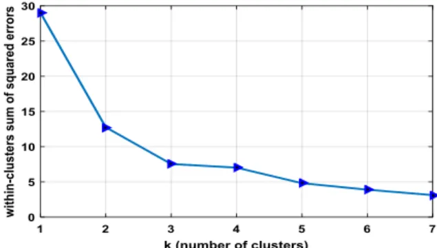
In order to illustrate the performance of the proposed detection/compensation scheme, a real-world data set for evaluation is selected [23]. This data set consists of labeled samples in both normal and faulty cases. The first step is to determine the number of clusters of faulty/sub-health states. Hence, in clustering step the samples of normal state are excluded. The remaining data comprises of three different faulty cases, but this number is hidden from the classifier/detector agent. Therefore, In Fig. 3, within-clusters SSE for each data point in data set have been calculated for different values of 𝐾 ranges from 1 to 7.
It is evidence, with increasing K the SSE is being decreased continuously. But, the value K=3 is a key point in which the fluctuation in SSE is very negligible thereafter. As a result, the number of sub-health (faulty) states is estimated as 3. It should be noted that the remaining parameters that must be estimated using input data set are μ and λ which is out of scope of this paper.
In order to determine the clusters and centroid points, the K-means algorithm is applied over the training data set using Weka which is a collection of ML algorithms for data mining tasks. For declaration, the result of clustering in terms of two sample KPIs, i.e., throughput and RSRP, is illustrated in Fig. 4. Also, the extracted centroid points correspond to 3 clusters in terms of 6 KPIs is given in Table III.
Figure 3. Optimal number of clusters 𝐾 using Elbow method
Figure 4. 𝐾-Means clustering in terms of throughput and RSRP attribute
TABLE III. CLUSTER'S CENTROID POINTS Attribute Cluster1 Cluster2 Cluster3
Retainability 0.9951 0.9309 0.944
HOSR 0.9876 0.9229 0.849
RSRP -77.4961 -72.6767 -65.8896
RSRQ -18.1811 -18.1279 -19.4155
SINR 12.6378 7.0127 13.6656
Throughput 89.1056 68.7371 175.0776
In compensation step, knowing the number of sub-health states, a system with three sub-sub-health states, namely {𝑠1, 𝑠2, 𝑠3} is considered as shown in Fig. 2.
Thus, the outage and optimal states are represented by 𝑠0 and 𝑠4, respectively. For simplicity, we assume that
there is no any transition from state 𝑠1 and 𝑠3 and vice
versa. In fact, we can move to states 𝑠1, 𝑠2, 𝑠0 and 𝑠4
from state 𝑠1.
By estimating MDP parameters (using the given dataset in both normal and faulty states), extracting the optimal action in each sub-health states is straight forward. However, in order to describe the advantage of the proposed scheme in compensation process and action policy extraction, we consider four scenarios. The parameters of each scenario are given in Table IV.
TABLE IV. TRANSITION RATES
Parameter Value
[𝜆𝑐04, 𝜆 𝑐 14, 𝜆
𝑐 24, 𝜆
𝑐 34]
𝑺𝒄𝒆𝒏𝒂𝒓𝒊𝒐 𝟏: {𝜆𝑐𝑖4}𝑖=03 = 1/8 𝑺𝒄𝒆𝒏𝒂𝒓𝒊𝒐 𝟐: {𝜆𝑐𝑖4}𝑖=03 = 1/8 𝑺𝒄𝒆𝒏𝒂𝒓𝒊𝒐 𝟑:
{𝜆𝑐𝑖4}𝑖=03 = [ 1/8 ,1/7 ,1/6 ,1/5 ] 𝑺𝒄𝒆𝒏𝒂𝒓𝒊𝒐 𝟒:
{𝜆𝑐𝑖4}𝑖=03 = [ 1/8 ,1/5 ,1/3 ,1/2 ] 𝜆𝑡𝑖𝑗
for all possible (𝑖, 𝑗) 1/8, for all scenarios 𝜇𝑑𝑐,𝑎𝑖𝑗 1
for all possible (𝑖, 𝑗)
6, for all scenarios
𝜇𝑑𝑐,𝑎
2
𝑖𝑗
for all possible (𝑖, 𝑗)
10, for all scenarios
𝜇𝑐 1/12, for all scenarios
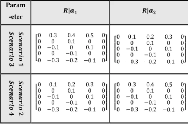
TABLE V. REWARDS ASSIGEND IN DIFFERENT SCENARIOS
Param
-eter 𝑹|𝒂𝟏 𝑹|𝒂𝟐
𝑺𝒄 𝒆𝒏 𝒂 𝒓𝒊 𝒐 𝟏 𝑺𝒄 𝒆𝒏 𝒂 𝒓𝒊
𝒐 𝟑 [
0 0 0 0 0 0.3 0 −0.1 0 −0.3 0.4 0.1 0 −0.1 −0.2 0.5 0 0.1 0 −0.1 0 0 0 0 0] [ 0 0 0 0 0 0.1 0 −0.1 0 −0.3 0.2 0.1 0 −0.1 −0.2 0.3 0 0.1 0 −0.1 0 0 0 0 0] 𝑺𝒄 𝒆𝒏 𝒂 𝒓𝒊 𝒐 𝟐 𝑺𝒄 𝒆𝒏 𝒂 𝒓𝒊
𝒐 𝟒 [
0 0 0 0 0 0.1 0 −0.1 0 −0.3 0.2 0.1 0 −0.1 −0.2 0.3 0 0.1 0 −0.1 0 0 0 0 0] [ 0 0 0 0 0 0.3 0 −0.1 0 −0.3 0.4 0.1 0 −0.1 −0.2 0.5 0 0.1 0 −0.1 0 0 0 0 0]
Moreover, the rewards assigned to actions a_1 and a_2 are demonstrated in rewards-matrix R as shown in TABLE V. Since the rewards depend only on the actions in a given state and we execute the actions only in sub-health states, the reward values are set to be non-zero for the three sub-health states. Transition from a sub-health state to the optimal state, which is called recovery transition, takes the positive reward. This is also set for transition from a sub-health state to another sub-health state with lower index which has superior condition. On the contrary, transition to outage or another sub-health state with an inferior condition brings a negative reward.
In Scenario 1, more reward is allocated to a given sub-health state to move to the optimal state when action 𝑎1 is executed while the smaller
detection-compensation time is made. This can resemble the situation where achieving better quality of service (QoS) has the higher priority. Scenario 2 simulates a reverse situation, i.e., when the performance efficiency is our concern instead of recovery time. Thus, in scenario 2, the system consumes fewer resources for recovery while a given state takes more transition time to move to the optimal state. Hence, detection-compensation time is longer when action 𝑎2 is selected.
In scenarios 1 and 2, 𝜆𝑐𝑖4 (𝑖 = 0,1,2,3) are defined to be
the same. The rewards assigned to Scenarios 3 and 4 are similar to them in Scenarios 1 and 2, respectively. However, the transition rates from sub-health states to outage state in both scenarios (i.e., Scenarios 3 and 4) are selected from four different values as depicted in Table IV. This means that the probability of occurring outage in worse sub-health condition is more probable as it is supposed to be in real situations. The other parameters are assumed to be the same in all scenarios, as demonstrated in Table IV.
We consider two algorithms to choose the policy 𝜋(𝑎|𝑠) which are denoted by optimal and random policies. The optimal policy is the solution to the optimization Problem 1. While in the random policy algorithm, we randomly opt one of the actions 𝑎1 or 𝑎2
with uniform distribution in a given state. In Fig. 5, we depict the average rewards obtained in both optimal and random policies for four considered scenarios. Evidently, the rewards achieved by using the optimal policy are significantly higher than them obtained by the random policy. However, some important information about the behavior of the system and the proposed optimum policy can be extracted from these
observations that are explained as follows. As observed from TableV, more rewards are assigned to the actions 𝑎1 with short recovery time in Scenario 1, while, action
𝑎2 with long recovery time takes the bigger rewards in
Scenario 2. On the other hand, the critical-failure rates of 𝜆𝑐𝑖𝑗 in both scenarios are small and the same.
Therefore, in Scenario 2, the system has enough time to recover from sub-health states into optimal state and consequently the average reward is more than that of other scenarios. In Scenario 3, although 𝜆𝑐𝑖𝑗 increases in worse sub-health state, the action 𝑎1 with short
recovery time has more chance to be selected in sub-health states. As a result, the expected recovery time is short and most of the time the system can recover before going to outage. The reason is that the average reward is similar to Scenario 1. In Scenario 4, the situation is different. The recovery time is long due to choosing the action 𝑎2, and the system may go into
worse sub-health states (and even outage) with more probability in the meantime. Increase in rate of 𝜆𝑐𝑖𝑗 with
going into worse sub-health states makes the condition even worse. As a result, we can see a significant loss in achieved reward in comparison to Scenario 2.
The average recovery time 𝑇𝑎𝑣𝑔𝑟𝑒𝑐𝑜𝑣𝑒𝑟𝑦 in the sub-health state is obtained as
𝑇𝑎𝑣𝑔𝑟𝑒𝑐𝑜𝑣𝑒𝑟𝑦= ∑ 𝑝(𝑠𝑖) ∑ 𝜇𝑑𝑐,𝑎𝑗
𝑖0 𝜋(𝑎 𝑗|𝑠𝑖). 2
𝑗=1 3
𝑖=1
𝑇𝑎𝑣𝑔𝑟𝑒𝑐𝑜𝑣𝑒𝑟𝑦 in four considered scenarios are depicted in Fig. 6. Obviously, the optimal policy in Scenarios1 and 3 creates substantial short recovery time. However, if we want to achieve more reward in Scenarios 2 and 4, we need to execute action 𝑎2 which makes long
recovery time. Therefore, the increase in average recovery time of Scenario 2 is completely normal. But Scenario 4 needs more explanation. In fact, due to the increasing rate of critical failure 𝜆𝑐𝑖𝑗 in worse sub-health
states, almost all the successful system recoveries take place in sub-health state 1 and after that in sub-health stat 2 with less probability but yet more than sub-health 3. Therefore, the average recovery time is smaller than Scenario 2.
Figure 5. Average rewards achieved by proposed optimal policy/random policy in four considered scenarios
Figure 6. Average recovery time for proposed optimal policy/ random policy in four considered scenarios
Figure 7. Sub-health state probability in 4 scenarios (optimal policy) Fig. 7 depicts the probability of being in sub-health states in Scenarios 1 to 4, when the proposed optimal policy is applied and the rewards defined in Table V are utilized. As shown in Fig. 7, the sub-health state can recover fast and hence move to the optimal state rapidly in Scenario 1. Evidently, the probability of being in different states decreases steadily as transferring from state 1 to state 3 in scenarios 1, 2, and 3. This behavior becomes more drastic in scenario 3 due to the augmented critical failure rate from 𝜆𝑐14 to 𝜆𝑐34. In the
contrary, the SH agent recovers from sub-health states with more recovery time while utilizes fewer resources in Scenario 2. In fact in this scenario, SH agent acts more efficient in terms of consuming the recourses and therefore, the recovery time is of the secondary importance. As a result, the SH agent may choose the action with longer (or shorter) average recovery time in a given sub-health state that tends to increase (or decrease) the probability of being in worse (or best) sub-health states. Regarding the tendency of system in choosing one of the possible actions, the Scenarios 2 and 4 behave similarly. In Scenario 4, the critical-failure rate of 𝜆𝑖𝑗𝑐 in sub-health 2 is much more than
health 1 and in health 3 is much more than sub-health 1 and 2. The effect of critical-failure rate is dominant and it can be seen that the probability of being in sub-health states decreases from sub-health 1 to 3.
V. COCLUSION
We presented a context-aware proactive SH scheme utilizing machine learning algorithms which includes detection and compensation processes. 𝐾 -means clustering were employed for the detection process. This algorithm is employed when the number of clusters or equivalently the number of faulty states are known. We also proposed a framework to analyze the system stochastically and investigate the impact of actions executed in sub-health states of a SH process. Using discrete-time Markov Decision Process, a model was suggested analytically to find out the optimal actions before the outage happens. The proposed framework supports any special fault or failure scenario and any situation in which the system may tend to go to a sub-health state. Since our proposed model was inherently a continuous-time Markov chain, we applied discretizing process to assess the model in discrete-time behavior. Furthermore, an equivalent LP formulation corresponding to considered optimization problem is employed to obtain the optimal policy. We used a real world data base for detection process and computed the number of sub-health states. We also considered four different scenarios for compensation phase. We numerically analyzed the results for various rewards and indicators of the performance, e.g., average recovery time to compare our proposed optimal policy with random action selection policy. The results demonstrate that the suggested analytical model is beneficial and proposed optimal policies perform well in contrast to random action selection policies.
REFERENCES
[1] M. Shafi et al., "5G: A Tutorial overview of standards, trials, challenges, deployment, and practice," in IEEE Journal on Selected Areas in Communications, vol. 35, no. 6, pp. 1201-1221, Jun. 2017.
[2] I. Afolabi, T. Taleb, K. Samdanis, A. Ksentini and H. Flinck, "network slicing and softwarization: A survey on principles, enabling technologies, and solutions," in IEEE Communications Surveys & Tutorials, vol. 20, no. 3, pp. 2429-2453, third quarter 2018.
[3] Y. Mao, C. You, J. Zhang, K. Huang and K. B. Letaief, "A survey on mobile edge computing: The communication perspective," in IEEE Communications Surveys & Tutorials, vol. 19, no. 4, pp. 2322-2358, fourth quarter 2017.
[4] J. Moysena and L. Giupponib, "From 4G to 5G: Self-organized network management meets machine learning,” Computer Communications, vol. 129, pp. 248-268, Sep. 2018.
[5] "Wireless technology evolution towards 5G: 3GPP Release 13 to Release 15 and Beyond," a White Paper Published by 5G Americas, February 2017.
[6] L. Jorguseski, A. Pais, F. Gunnarsson, A. Centonza and C. Willcock, "Self-organizing networks in 3GPP: standardization and future trends," in IEEE Communications Magazine, vol. 52, no. 12, pp. 28-34, Dec. 2014.
[7] H. Gacanin and A. Ligata, "Wi-Fi self-organizing networks: challenges and use cases," in IEEE Communications Magazine, vol. 55, no. 7, pp. 158-164, 2017.
[8] A. Imran, A. Zoha, and A. Abu-Dayya, "Challenges in 5G: how to empower SON with big data for enabling 5G, " IEEE Network, vol. 28, no. 6, pp. 27–33, 2014.
[9] N. Bhushan et al., "Network densification: the dominant theme for wireless evolution into 5G," in IEEE Communications Magazine, vol. 52, no. 2, pp. 82-89, February 2014.
[10] P. V. Klaine, M. A. Imran, O. Onireti and R. D. Souza, "A survey of machine learning techniques applied to self-organizing cellular networks," in IEEE Communications Surveys & Tutorials, vol. 19, no. 4, pp. 2392-2431, fourth quarter 2017.
[11] A. Zoha, A. Imran, A. Abu-Dayya and A Saeed, “A machine learning framework for detection of sleeping cells in LTE network,” in Proceedings of the Machine Learning and Data Analysis Symposium, Mar. 2014.
[12] S. Fortes, A. Aguilar Garcia, J. A. Fernandez-Luque, A. Garrido and R. Barco, "Context-aware Self-Healing: user equipment as the main source of information for small-cell indoor networks," in IEEE Vehicular Technology Magazine, vol. 11, no. 1, pp. 76-85, Mar. 2016.
[13] M. Shruti, B. Yagnik, D. Binod, and C. Agrawal, "Analyzing the extracted file metadata evidences from suspicious nodes in DFXML format using clustering techniques," in International Journal of Applied Engineering Research, vol. 13, no. 23, pp. 16279-16281, 2018.
[14] S. Chernov, D. Petrov and T. Ristaniemi, "Location accuracy impact on cell outage detection in LTE-A networks," 2015 International Wireless Communications and Mobile Computing Conference (IWCMC), Dubrovnik, 2015, pp. 1162-1167.
[15] A. Asghar, H. Farooq and A. Imran, "Self-Healing in emerging cellular networks: review, challenges, and research directions," in IEEE Communications Surveys & Tutorials, vol. 20, no. 3, pp. 1682-1709, third quarter 2018.
[16] A. Gómez-Andrades, R. Barco, P. Muñoz and I. Serrano, "Data analytics for diagnosing the rf condition in self-organizing networks," in IEEE Transactions on Mobile Computing, vol. 16, no. 6, pp. 1587-1600, 1 June 2017.
[17] Palacios, I. de-la-Bandera, A. Gómez-Andrades, L. Flores and R. Barco, "Automatic feature selection technique for next generation self-organizing networks," in IEEE Communications Letters, vol. 22, no. 6, pp. 1272-1275, Jun. 2018.
[18] A. Tall, R. Combes, Z. Altman and E. Altman, "Distributed coordination of self-organizing mechanisms in communication networks," in IEEE Transactions on Control of Network Systems, vol. 1, no. 4, pp. 328-337, Dec. 2014.
[19] P. Muñoz, R. Barco, I. Serrano and A. Gómez-Andrades, "Correlation-based time-series analysis for cell degradation detection in SON," in IEEE Communications Letters, vol. 20, no. 2, pp. 396-399, Feb. 2016.
[20] Y. Kumar, H. Farooq and A. Imran, "Fault prediction and reliability analysis in a real cellular network," 2017 13th International Wireless Communications and Mobile Computing Conference (IWCMC), Valencia, 2017, pp. 1090-1095.
[21] H. Farooq, M. S. Parwez and A. Imran, "Continuous time Markov chain based reliability analysis for future cellular networks," 2015 IEEE Global Communications Conference (GLOBECOM), San Diego, CA, 2015, pp. 1-6.
[22] K. P. Murphy, "Machine Learning: A probabilistic perspective," The MIT Press, 2012.
[23] R. Barco, Available [Online]:
http://webpersonal.uma.es/~RBARCO/home.html
[24] A. Jensen, “Markoff chain as an aid in the study of Markoff processes,” in Skandinavisk Aktuarietidskrift, vol. 36, pp. 87-91, 1953.
[25] J. McMahon, "Time-dependence in Markovian decision processes," Thesis for the degree of Doctor of Philosophy in Applied Mathematics, University of Adelide, School of Applied Mathematics, Sep. 2008.
[26] R. Joda and M. Zorzi, "Access policy design for cognitive secondary users under a primary Type-I HARQ process," in IEEE Transactions on Communications, vol. 63, no. 11, pp. 4037-4049, Nov. 2015.
[27] R. Joda and M. Zorzi, “Centralized access policy design for two cognitive secondary users under a primary ARQ process,” in Proc. IEEE ICC, Jun. 2014, pp. 268–273.
AUTHORS'INFORMATION
Shirin Nikmanesh received her B.Sc. in computer engineering (software) in 2013 from Islamic Azad University, Boroujerd Branch, Iran. She is currently pursuing the M.Sc. degree in the Department of Technology and Engineering, Islamic Azad University, Central Tehran Branch, Tehran, Iran. Her current research mainly focuses on artificial Intelligence, 5G and Self-organizing Networks.
Mohammad Akbari received
his B.Sc. in Electrical
Engineering in 2008 from Tabriz University, Tabriz, Iran, and the M.Sc. and Ph.D. degrees both from Iran University of Science and Technology (IUST), Tehran,
Iran in 2010 and 2016
respectively. During 2010-2017 he was a senior system designer at Kavoshcom Asia Research Group, Tehran, Iran. In 2017, he joined as an assistant professor to the Department of Communication Technology, ICT Research Institute (ITRC), Tehran, Iran. His current research interests span topics in telecommunication system and networks including 5G, self-organizing networks and application of machine learning techniques in wireless communication.
Roghayeh Joda (M14) received the B.Sc. degree in Electrical
Engineering from Sharif
University of Technology, Tehran, Iran, in 1998, and the M.Sc. and Ph.D. degrees in Electrical Engineering from the University of Tehran, Tehran, Iran, in 2001 and 2012, respectively. During her Ph.D. studies, she has been a Visiting Scholar at the Polytechnic Institute of NYU, Brooklyn, NY, USA. She has worked as a Research Associate at University of Tehran, Tehran, Iran, from November 2012 to July 2013 and then as a Postdoctoral Fellow at University of Padova, Padova, Italy, from September 2013 to July 2014. She is currently a research assistant professor at Iran Telecommunication Research Center, Tehran, Iran. Her current research interests include network information theory, source, channel and network coding, resource allocation, optimization, cognitive radio networks, self-organized networks, 5G networks, caching and machine learning algorithms.
![TABLE I. K EY PERFORMANCE INDICATORS USED IN DETECTION PROCESS [23]](https://thumb-us.123doks.com/thumbv2/123dok_us/8369458.2222820/3.893.252.623.107.294/table-i-ey-performance-indicators-used-detection-process.webp)