Major depression has been a worldwide concern and poses a threat to both the mental and physical health of its sufferers. Currently, practitioners rely on standard surveys and questionnaires to diagnose depression. However, these means of diagnosis are costly and come into play after the worsening of the depression rather than offering an easily accessible means of early detection. Using the CLEF/eRisk 2017 dataset, this thesis combined basic natural language techniques including TF-IDF, the state-of-art
Word2Vec model, LIWC features and a manually built sentiment dictionary. A logistic regression classifier achieved an F1 score of 0.6207 using the whole test data. This approach might offer some contributions to future research which addresses the thorny issue of depression screening.
Headings:
by Chenlu Meng
A Master’s paper submitted to the faculty of the School of Information and Library Science of the University of North Carolina at Chapel Hill
in partial fulfillment of the requirements for the degree of Master of Science in
Information Science.
Chapel Hill, North Carolina May 2020
Approved by
TABLE OF CONTENTS
TABLE OF CONTENTS ... 1
INTRODUCTION ... 3
1.1 Social Media and Depression Detection ... 3
1.2 Research Objective ... 5
LITERATURE REVIEW ... 6
2.1 Social Media and Mental Disorders ... 6
2.2 Overview of Previous Work ... 7
2.3 Data Collection and Ethical Issues ... 8
2.4 CLEF/eRisk 2017 Task ... 10
2.5 Other Works in Mental Disorder Detection ... 11
DATASET ... 19
3.1 Overview of Data ... 19
3.2 Class Imbalance ... 21
METHODS ... 25
4.1 Preprocessing ... 25
4.2 Exploratory Data Analysis ... 28
4.2.1 Structural Features ... 28
4.2.2 Part-of-Speech Tagging ... 32
4.2.3 Word Proportion ... 33
4.3 Feature Selection ... 34
4.3.1 Structural Features ... 36
4.3.2 Topic Modeling ... 36
4.3.3 Polarity ... 38
4.3.4 TF-IDF and Count Vectorizer ... 40
4.3.5 Phrase Modeling and Word2Vec ... 42
4.3.6 LIWC Features ... 45
4.3.7 Lexical Features ... 49
RESULTS ... 52
5.2 Classifiers ... 54
DISCUSSION ... 60
CONCLUSION ... 62
APPENDIX A ... 66
APPENDIX B ... 68
INTRODUCTION 1.1 Social Media and Depression Detection
Major depressive disorder, known as depression, is marked by a distinct change of mood to sadness or irritability, along with a few psychophysiological changes (Belmaker & Agam, 2008). It is among the most prevalent mental disorders impacting people. In the United States, the lifetime incidence of depression is more than 9% in men and 17% in women (Hasin, Goodwin, Stinson, & Grant, 2005). The vast number of patients are affected not only psychologically but also physically; in fact, many physical disorders are more prevalent in individuals with severe mental disorders including major depression (De Hert et al., 2011). In addition to the physical sufferings due to major depression, public stigma also has a major impact on depressed individuals and may interfere with various aspects of life (Rüsch, Angermeyer & Corrigan, 2005). Social withdrawal due to this impact can lead to many turning to social media websites and forums for help. Online forums can provide patients with information pertaining to depression relief and
additional emotional support (Prescott, Hanley & Ujhelyi, 2017). Depression has led to world-scale concerns with its negative impacts in health and social problems. Effective ways to mitigate the negative influences are in urgent need.
Association [APA], 2013). Formal diagnosis takes the form of passive observation, however, many patients fail to seek medical advice until the worsening of the situation for various reasons, which may result in delayed intervention. Nearly 50% of people did not seek medical advice during a depressive episode because they lack trust in the effectiveness of the treatment, associate shame or weakness with depression, seek social support from family and friends, or had negative experience with doctors (Rondet et al., 2015). Other studies reported that it was financial barriers that hindered people from seeking treatment (Kessler et al., 2001). Le and Boyd (2006) proved that early
intervention can prevent depression from developing into a clinical level. Kessler et al. (2007) confirmed this opinion by stating that timely interventions with early‐stage mental disorders might help reduce the level of severity of primary disorders, and also delay or avoid the onset of accompanying disorders.
By making use of the large scale of social media data, language patterns can act as an indicator to the mental health state, even contributing to the early detection of
1.2 Research Objective
This study aims to use text mining and Natural Language Processing (NLP) methods to improve the detection of depression using textual data. Such a classifier would have the potential to act as a preliminary screening method before depression diagnosis. The following questions are to be answered in the study:
1. What are the language patterns of individuals with depression in online communities? 2. What textual features contribute most to the detection of users with depression?
LITERATURE REVIEW
In this chapter, relevant works on detection of mental disorders using social media data are discussed. The insights derived from previous works can help identify the gap and construct a new approach for this study.
2.1 Social Media and Mental Disorders
Social media sites, defined as web-based services on which individuals can construct and maintain connections with other users (Boyd & Ellison, 2007), enable people to have social interactions regardless of their physical distance. Pew Research Center (PRC, 2019, para. 4) reported that as of 2019, among American adults, 72% used at least one social media site, 69% used Facebook, 37% used Instagram, 22% used Twitter and 11% used Reddit. The widely used social media makes it possible for every user to express themselves in a convenient and timely way. The user-generated
information integrating personal thoughts and social behavior can reflect the actual emotional and mental state of users, rather than the idealized personalities users want to create (Back et al., 2010).
patients with depression and schizophrenia are both likely to overestimate the
stigmatizing attitudes towards them in the community. The fear of stigma might prevent patients from sharing or discussing their conditions with their family and friends. By contrast, social media allows people to connect with others with common experiences and opinions without revealing personal information. Rizvi, Kane, Correll, and Birnbaum (2015) found out that social media such as Facebook and Twitter was utilized by youth impacted by mental disorders to discuss their symptoms and decide whether to seek care especially during the early onset of their disorders. De Choudhury and De (2014) studied mental health disclosure on the popular social media Reddit and found that users
explored diverse topics ranging from the daily grind to diagnosis and treatment on social media.
2.2 Overview of Previous Work
Plenty of researchers were interested in the massive data related to mental disorders available on social media. According to 75 papers associated with mental disorder detection via social media from 2013 to 2018, the most popular social media site leveraged by researchers was Twitter, followed by Reddit, Sina Weibo, Facebook and Instagram, while the most studied mental disorder or related symptoms was depression, followed by suicidal ideation, schizophrenia and eating disorder (Chancellor & De Choudhury, 2020).
associated with depression by Rodriguez, Holleran, and Mehl (2010). In addition, depressed users tend to use more personal pronouns (e.g., I) and verbs in
continuous/imperfective/past tenses (Smirnova et al., 2018). As for differences in behavior patterns, De Choudhury, Counts, and Horvitz (2013) included social
engagement features in their approach to detect depression via Twitter social engagement features, namely, normalized number of posts, proportion of reply posts, fraction of retweets, proportion of links shared, fraction of question-centric posts (measuring user tendency to gain information from Twitter community).
2.3 Data Collection and Ethical Issues
Several methods have been utilized to collect data for automatic detection of mental disorders. To obtain the social media data of people with mental disorders, some researchers recruited participants with crowdsourcing. For instance, in a study to predict the onset of depression with Twitter data, De Choudhury et al. (2013, April) gathered participants located in the United States through Amazon’s Mechanical Turk. A total number of 1,583 crowdworkers answered a standard clinical depression survey, follow-up questions about depression experiences and demographics. Among these participants, 637 agreed to provide their Twitter feeds for the research. Participants who took less than two minutes to complete the survey or showed an inconsistency in responses of two screening tests were eliminated. The primary screening tests was Center for
before the survey were included, so that the dataset could contain a reasonably long history of social media data before the onset. The final dataset consisted of 476
participants. Individuals scoring positive in the primary screening test were assigned to the positive class and the rest to the negative. For users in the positive class, Twitter data was collected dating from the reported onset up to one year. For users in the negative class, Twitter data was collected dating from the survey date up to one year. Other researchers such as (Coppersmith et al., 2015) searched self-reported diagnoses of depression or Post Traumatic Stress Disorder (PTSD) from Twitter to create the dataset used in the CLPsych2015 task. Statements such as “I was just diagnosed with X” where X stood for depression or PTSD were used to identify Twitter users with depression or PTSD. After the misleading statements such as jokes or quotes were removed by a human annotator, the remaining users made up the diagnosed group of depression and PTSD. A random selection of Twitter accounts without mention of these diagnoses constituted the control group. Then the most recent 3,000 public tweets of each user were collected. Similarly, Yates, Cohan, and Goharian (2017) created the Reddit Self-reported Depression Diagnosis dataset by identifying Reddit users who posted “I was just diagnosed with depression”. Users with less than 100 posts before the diagnosis post were discarded. Three layperson annotators viewed the remaining posts to get rid of false positive posts (e.g., “if I was diagnosed with depression”) and only users with at least two positive annotations were included in the diagnosed group. The control group was
The easy access to a large-scale of social media data to detect mental disorders brings about some ethical issues. While the social media detection system can serve as a way of crisis intervention, whether and when users prefer to be notified or “saved” is a critical issue. Another possible application is to transform the system into a preliminary screening approach before clinical diagnosis of depression. The concerns about data security and privacy arise along with the opportunity. A common method to solve this problem is to anonymize user information. For example, Coppersmith et al. (2015) replaced user names, URLs and any other metadata that didn’t match the whitelisted entries that have minimal risks of revealing user identification (e.g., number of friends, followers, favorites, time zone) with a seemingly-random group of characters, so that content creators won’t be able to be identified.
2.4 CLEF/eRisk 2017 Task
The dataset for this study was created by Losada, Crestani & Parapar (2017) and has been utilized in CLEF/eRisk 2017 task which focuses on early risk detection of depression. This dataset was collected from Reddit by identifying depressed users with statements such as “I was diagnosed with depression”, while the control group consisted of a random selection of Reddit users. While the details of this dataset will be explained in the section 3, Dataset, in this section I review the methods of participants of this detection task.
user, stylometric features contain lexicon volume, average number of words per post, number of sentences per message and number words per sentence, while morphological features contain proportions of parts of speech (POS). The classifier built by Trotzek, Koitka, and Friedrich (2018) achieved the best F1 score of 0.64 during CLEF/eRisk 2017 and a F1 score of 0.73 after all the ground truth of test data was released. The best F1 score of Trotzek et al. (2018) was achieved with linguistic metadata features and Logistic Regression (LR). Linguistic features were based on a concatenation of the text and title field of each message, consisting of word and grammar usage, readability and metadata. Word and grammar usage features included average occurrences of past tense verbs, personal pronouns, possessive pronouns, the word “I” , and hand-picked phrases such as “my anxiety” and “my depression”. Readability, the complexity of written text (Trotzek et al., 2018), was calculated by the average of Flesch Reading Ease (FRE) (Flesch, 1948), Linsear Write Formula (LWF) (Christensen, G. J. ,n.d.) and New Dale-Chall Readability (DCR) (Dale & Chall, 1948) (Chall & Dale, 1995). Metadata features included average month of the writings, text length and title length. Trotzek et al. (2018) also experimented with the further developed version of Word2Vec, fastText, published by Facebook
(Joulin, Grave, Bojanowski, and Mikolov, 2016), and GloVe published by Stanford NLP group (Pennington, Socher, and Manning, 2014), but these features didn’t perform as well as the linguistic metadata features.
2.5 Other Works in Mental Disorder Detection
utilizing CLEF/eRisk 2017 dataset, this section will be focused on other works of detecting mental disorders. The summarized features, approaches and algorithms are listed in Table 1.
To predict depression via Twitter data collected by crowdsourcing, De Choudhury et al. (2013, June) utilized behavioral attributes relating to social engagement, emotion, linguistic styles, egocentric network, depression language and demographic features with . Social engagement was computed based on the tweets of each user per day. It consisted of five measures defined by De Choudhury et al. (2013, April), namely,
normalized number of posts, proportion of reply posts, fraction of retweets, proportion of links shared, fraction of question-centric posts (measuring user tendency to gain
information from Twitter community). The sixth social management feature was normalized difference in number of postings made between night window (9PM-6AM) and day window (6:01AM-8.59PM). Egocentric network features were calculated on three levels, node properties, dyadic properties and network properties. Node properties measured the number of followers and followees of a user. Dyadic properties measured how many times a user responded to another user. Network properties measured the network structures such as the ratio of counts of edges to the count of nodes for a user where edges stand for links between nodes. Linguistic Inquiry Word Count (LIWC) by Pennebaker et al. (2007) was used to compute positive affect (based on positive emotion category of LIWC), negative affect (based in negative emotion category of LIWC) and linguistic styles (based on LIWC categories such as articles, auxiliary verbs and
word stems, with each word or word stem belonging to one or more word categories (e.g., adverbs, religion, anxiety). Text is analyzed by calculating to what degree each category of words were used. In addition, Affective Norms for English Words (ANEW), constructed by Bradley and Lang (1999) and composed of a lexicon of words related to psychology, was used to compute activation and dominance. Activation means the intensity of an emotion (“terrified” shows higher activation than “scared”), and dominance means the degree of control of an emotion. For negative emotion, “anger” shows higher dominance than “fear”, while for positive emotion, “optimism” shows higher dominance than “relaxed”. Depression language features included depression lexicon and antidepressant usage. Depression lexicon was built by mining a 10% sample of “Mental Health” category of Yahoo! Answers and created a union of top 1% terms having highest pointwise mutual information and log likelihood ratio with regex “depress*”.
commit suicide” as negative phrases, and “I feel relaxed” and “I feel good” as positive phrases. The phrase-based dataset was further divided into training set (DB6) and test set (DB7). The proposed analyzer for text and emoticon was trained on DB1 and validated on DB2, DB5, DB6 and DB7. For text analyzer, the morphological analysis was
composed with mood lexicon and POS feature vector. Mood lexicon was based on Visual Sentiment Ontology (Borth, Ji, Chen, Breuel, & Chang, 2013) and SentiStrength
(Thelwall, Buckley, Paltoglou, Cai, & Kappas, 2010). Besides, to transform text into POS feature vectors, Kang et al. (2016) first identified each word’s POS and then transformed each sentence into a seven-dimensional feature vector (interrogative/interjection,
negative, adjective, noun, verb, adverb, and punctuation mark). For emoticon analyzer, Kang et al. (2016) calculated the sum of polarity scores by building a emoticon lexicon that translated emoticons to mood labels. For example, “:(“ belongs to mood “sad” with a polarity score of -4. Furthermore, an image dataset with 730 pictures labeled as positive, neutral, and negative created by Dan-Glauser and Scherer (2011) was divided into a training set (DB3) and test set (DB4). The image analyzer was trained on DB3 and
validated on DB4. This analyzer was composed with color composition (characteristics of colors in images and organization of combining these colors) and shape descriptors extracted from the image dataset. The three models (text, emoticon, image) to detect positive or negative moods achieved a F1 score of 0.8672 on DB7.
depressive dictionary learning (MDL) method to learn the latent and sparse
representation of users in terms of social network, user profile, visual features, emotional features, topic-level features, and domain-specific features. Social network features included number of tweets, number of followings and followers for each user. User profile features referred to genders, ages, relationships, and education levels returned by a big data platform for social multimedia analytics named bBridge (Farseev, Samborskii, and Chua, 2016). Visual features were obtained by extracting five-color combinations, brightness, saturation, cool color ratio and clear color ratio from users’ avatars.
To identify Bipolar Disorder (BD) and Borderline Personality Disorder (BPD) users on Twitter, Saravia, Chang, De Lorenzo, and Chen (2016) manually collected community portals (Twitter accounts that propagate information about a certain disorder) and selected users from the followers list who stated they were suffering from
“borderline”, “bpd” or “bipolar” in profiles as the BD and BPD group. The control group were obtained by randomly sampling users who didn’t express that they were suffering from BD or BPD. Saravia et al. (2016) used TF-IDF and pattern of life features with Random Forest classifier to detect BD and BPD Twitter users, where TF-IDF features yielded a precision of 96% for both BD and BPD models, and pattern of life features yielded a precision of 91% for BD model and 92% for BPD model. Pattern of life features included age, gender derived from the model proposed by Sap et al. (2014), polarity features and social features. Sentiment140 API1 was used to label each tweet as positive, neutral or negative. The polarity labels were transformed into five affective features of users, namely, positive ratio (percentage of positive tweets), negative ratio (percentage of negative tweets), positive combo to capture mania emotion (number of positive posts appearing more than 2 times continuously within 30 minutes), negative combo to capture depression emotion (number of negative posts appearing more than 2 times continuously within 30 minutes), flip ratio to measure emotional unstableness (number of times when posts with different polarity of positive or negative appeared more than 2 times continuously within 30 minutes). Social features included frequency of daily posts, percentage of posts containing mention of another user, number of users mentioned more than three times, number of unique users mentioned.
The most common features in detection of mental disorders included linguistic features and social activities, emotion dictionaries such as LIWC and ANEW, TF-IDF vectors and word embeddings such as Glove. The classifiers yielding good performances on different datasets included Support vector machine, Logistic Regression, and Random Forest.
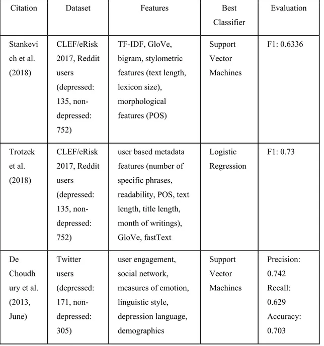
Table 1: Previous studies in detection of mental disorders via social media
Citation Dataset Features Best
Classifier
Evaluation
Stankevi ch et al. (2018) CLEF/eRisk 2017, Reddit users (depressed: 135, non-depressed: 752) TF-IDF, GloVe, bigram, stylometric features (text length, lexicon size), morphological features (POS) Support Vector Machines F1: 0.6336 Trotzek et al. (2018) CLEF/eRisk 2017, Reddit users (depressed: 135, non-depressed: 752)
Shen et al. (2017) Twitter users (depressed: 1,402, non-depressed: > 300 million)
social network, user profile, avatar visual features, measures of emotion, topic modeling, domain-specific lexicon Multimodal Dictionary Learning F1: 0.85 Kang, Yoon, and Kim (2016) Twitter (experiment ed on 7 datasets, to detect depressive moods)
text (mood lexicon, morphological feature vector), emoticon lexicon, image (color composition, SIFT descriptors) Support Vector Machines F1: 0.8672 Saravia et al. (2016) Twitter users (bipolar disorder: 203, borderline disorder: 278, control group: 548))
DATASET 3.1 Overview of Data
The dataset from the CLEF/eRisk 2017 shared task collected by Losada et al. (2017) was chosen as the dataset for this study. This is a labeled dataset consisting of posts of depressed and non-depressed Reddit, an online community where users can start threads, comments on posts and vote submissions, users. The long-history (the mean range of dates from first submission to latest submission for each user was more than 500 days) of posts in this dataset suits the purpose of this research perfectly.
were truly depressed users in the control group, but it was expected that these cases could be neglected (Losada et al.,2016). Under the limitation of Reddit’s policy that up to 1000 posts and 1000 comments can be crawled, as many submissions as possible were
retrieved for each user. The posts with mention to diagnosis were removed from the dataset so that the classifier would not be centered on diagnosis expressions that the authors used to extract the depressed users. Users with less than 10 submissions were removed to make sure that there is enough data to be analyzed per user.
The dataset consists of textual submissions including “text” and “title”, where “text” stands for the contents of comments and posts, while “title” stands for titles of posts. No images were included in it but all URLs were kept. Depressed and
non-depressed users were further divided into a training set and test set. Submissions of each user in the training and test sets were grouped into 10 divisions called “chunks” in a chronological order. The X chunk of data accounts for submissions of all users in Xth
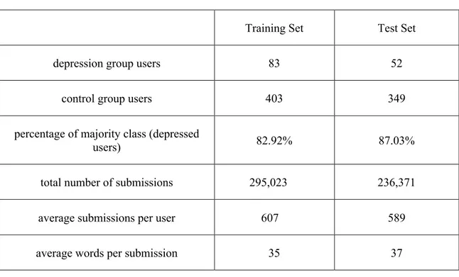
Table 2: A brief summary of training and test set
Training Set Test Set
depression group users 83 52
control group users 403 349
percentage of majority class (depressed
users) 82.92% 87.03%
total number of submissions 295,023 236,371
average submissions per user 607 589
average words per submission 35 37
3.2 Class Imbalance
Last section described how the data for was collected by Losada et al. (2017); in this section, I focused on the problem of class imbalance of the original dataset. Table 2 shows that the training set consists of 82.92% non-depressed users and 17.08% depressed users. With the object to correctly detect the minority class of depressed users,
appropriate methods and evaluation metrics should be adopted to deal with this problem. A common way to solve the problem of class imbalance is to resample the
imbalance, oversampling, can be further categorized as random oversampling and synthetic oversampling. Random oversampling refers to randomly duplicating existing minority class samples in order to increase the size of minority class in the training set (Shelke, Deshmukh, & Shandilya, 2017), but it has some limitations. Kaur and Gosain (2018) mentioned that the way of replicating existing minority samples may lead to the problem of overfitting. Synthetic Minority Oversampling (SMOTE), an oversampling method designed by Chawla et al. (2002), can create new instances of minority class by using the approach of k-nearest neighbors. However, the fact that this case is user-based rather than instance-based classification leads to several reasons why SMOTE sampling is not appropriate. Firstly, the length of the concatenated text of each user was much longer than that of a single post, thus the concatenated text may contain sentences of both positive and negative emotion. Besides, the personal writing style also makes it hard to form neighboring users using SMOTE oversampling methods since two depressed users might have different writing styles. These reasons make it hard to identify “neighbors” for a sample (concatenated text of a user).
Based on the above discussing about resampling methods, I adopted another approach to reduce the class imbalance problem, namely, cost-sensitive learning method. This method takes misclassification cost, instead of misclassification error, into
consideration. The cost-sensitive method prevents classifiers to be biased towards the majority class by imposing a cost penalty on the misclassification of minority class. The scikit-learn2 library in Python provides cost-sensitive learning option in several classifiers
via the “class_weight” argument. By assigning a higher weight to the minority class, the misclassification error for this class becomes larger when the algorithms are trained.
For a dataset with class imbalance, the evaluation metrics also need to be considered. Accuracy may lead to false judgment of the classifier, because by simply assigning all data to the majority class, accuracy is likely to be high (Visa, & Ralescu, 2005). In the scenario of depression detection based on textual data, the cost of missing one positive instance (the user is actually depressed, but is classified as non-depressed) is much higher than mistakenly classifying an individual with normal sadness as depressed. In other words, it costs more to miss a positive instance than falsely identify a negative instance. We need to get as many positive instances as possible with a relatively high precision. Therefore, F1 score can act as the primary evaluation metrics for this
classification task and recall and precision should also be reported for reference. F1 score is the harmonic mean of precision and recall. Precision measures the proportion of correctly identified positive instances in all predicted positive instances, while recall measures the proportion of correctly identified positive instances in all positive instances.
!"#$%&%'( =
#,-../,012 34/50363/4 7-83039/ 3580:5,/8#:11 7./43,0/4 7-83039/ 3580:5,/8
"#$;<< =
#,-../,012 34/50363/4 7-83039/ 3580:5,/8 #:11 7-83039/ 3580:5,/8=1 = ? ∗ 7./,383-5 ∗ ./,:117./,383-5 A ./,:11
(the number of predicted false positives divided by the total number of negative
instances) does not vary much when the number of the total number of negative instances is large. In contrast, PR curve displays the tradeoff between precision and recall, which is more useful when positive instances are rare.
METHODS 4.1 Preprocessing
The raw data is in the form of XML files, containing many symbols, punctuation marks, and URLs. I extracted and normalized the text data, then vectorized it for
classification.
Firstly I read the data from XML tags and built a data frame composed of four columns using the Pandas and Numpy libraries in Python as shown in Table 3. The second and third column were then combined as the “Text” column to represent all textual contents submitted by one user, resulting in a three-column data frame.
Table 3: Data frame columns of train and testing data Column 1 user id
Column 2 concatenated titles of posts for each user
Column 3 concatenated contents of comments and posts for each user
Column 4 true label of each user (“1” for depressed users, “0” for non-depressed users)
The preprocessing approach was conducted on the column “Text” (all textual contents including posts, comments and titles) in three different versions. These versions of clean text were prepared for different types of feature extraction.
libraries that score polarities, emoticons and punctuations matter. Thus these characters should be kept.
1. Remove all whitespace characters. Characters such as “\\n” occupy spaces but don’t change the meaning of the text.
2. Remove reddit-specific whitespace characters. “r/” and “u/” stands for a subreddit and a user respectively but don’t convey enough information for the classification task.
3. Remove URLs. Many users tend to include URLs in their online posts and
comments; although some words in these URLs might be helpful to the classification task, it is difficult to distinguish the meaningful ones from random strings, so the complete URLs were removed.
4. Expand text abbreviations. Online posts and comments consist of many text
abbreviations, these abbreviations were expanded into their full forms. Because this transformation was mainly to prepare the text for stop-word removal in a later step, ambiguous case “I’d” was transformed to “I” and “he’s” was transformed to “he” so that stopwords such as “would” or “had”, “is” or “was” were removed directly.
5. Convert text to lowercase characters. The lowercase text can reduce variations of words caused by capitalization, serving as a foundation of vectorization and feature extraction. For example, “That restaurant is REALLY good” should be converted to “that restaurant is really good”.
6. Use RegexpTokenizer3 to tokenize text, removing characters other than sentence
separators (!?.) and alphabetic characters. RegexpTokenizer compiles regular
expressions and removes unwanted characters before tokenizing a string. By passing r'[a-z\.\!\?]+' to RegexpTokenizer, only strings composed of lowercase alphabetic characters and sentence separators (!?.) were kept and tokenized.
7. Replace four or more consecutive repeating characters in a word with one character. Online posts and comments contain plenty of words using repeating characters to express strong feelings (e.g., “shiiiiiiiit”). These words need to be normalized for later vectorization and model building.
8. Join tokens together into strings with a space between each token.
9. Replace four or more consecutive repeating words in text with one word. Some users typed word duplicates by mistake or with intention. For instance, one post
encompasses “putt putt putt ... putt putt”, these rarely used words may bias the model.
The second version of clean text (tokenized sentences) was built upon “clean sentences” corpus. It was prepared for models using sentence corpus as input. For models capturing semantic meaning, the context of the word is important, thus completely
removing stop words should be avoided.
10. Replace four or more consecutive repeating punctuations with one punctuation. The
repeating punctuations express intense emotions but are not useful for building word vectors.
11. Conduct sentence segmentation using nltk.sent_tokenize4.
12. Tokenize and lemmatize words in each sentence. Lemmatization was chosen over
stemmer because lemmatized words are in their dictionary forms rather than stem
forms, which makes the interpretation easier. Lemmatization generates different normalization results for different parts of speech. To produce more accurate results, I set the order of lemmatization to be first verbs then nouns, so that words such as “caring” was transformed to “care” rather than “caring”.
13. Build a list for each user with lists of sentence tokens as items. For example, “i like
the room. the food was good too.” should be converted to [[‘i’,’like’,’the’,’room’],[‘the’,’food’,’was’,’good’,’too’]].
The third version of clean text (clean tokens) was built upon “tokenized
sentences” corpus. It was prepared for basic natural language processing techniques such as count vectorizer and Term Frequency Inverse Document Frequency (TF-IDF). All words were reduced to their basic roots in clean sentence corpus and now stop words were removed. Stop words are a set of words mostly commonly used in a language, in English, some examples are “the”,”a”,”of”.
14. Remove stop words using gensim.parsing.preprocessing.STOPWORDS and tokens
whose length were shorter than three.
15. Remove sentence separators (!?.).
4.2 Exploratory Data Analysis 4.2.1 Structural Features
Then an exploratory analysis was conducted on class distribution and other descriptive statistics of the dataset.
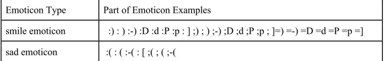
Wang and Castanon (2015), then extracted with regular expression. Then the proportion of all emoticons, smile emoticons and sad emotions were calculated for each class.
Table 4: Emotion types and examples
Emoticon Type Part of Emoticon Examples
smile emoticon :) : ) :-) :D :d :P :p : ] ;) ; ) ;-) ;D ;d ;P ;p ; ]=) =-) =D =d =P =p =]
sad emoticon :( : ( :-( : [ ;( ; ( ;-(
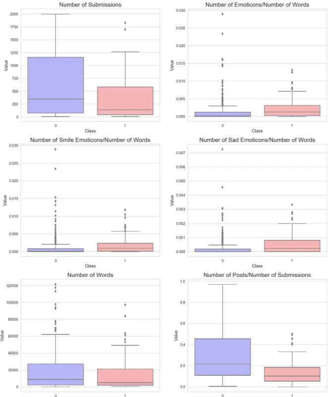
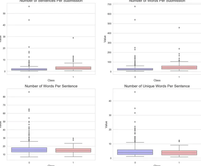
Structural features were calculated to visualize the difference in two classes and were extracted from concatenated text of each user. Features included number of submissions, proportion of all emoticon, smile emoticon and sad emoticon, number of words,
Figure 2: Structural features visualization of train data part 2 (1 stands for depressed, 0 stands for non-depressed)
Although Figure 1 and Figure 2 did not offer useful insights into feature engineering, it suggests some differences between depression and control group users:
2. The median proportions of all emoticons, smile emoticons, and sad emoticons of depressed users were all greater than that of non-depressed users. Depressed users tend to use more emoticons (both smile and sad ones) to express their emotions. 3. The median number of words of non-depressed users is only slightly larger than that of depressed users, which might imply that the number of words (text length) of depressed and non-depressed users are not significantly different.
4. The median proportion of posts (initiated threads) of depressed users is smaller than that of non-depressed users, implying that depressed users in this dataset were less likely to initiate a thread compared with non-depressed users.
5. Depressed and non-depressed users show similar number of sentences and words per submission.
6. Depressed and non-depressed users show similar number of words and unique words per sentence.
4.2.2 Part-of-Speech Tagging
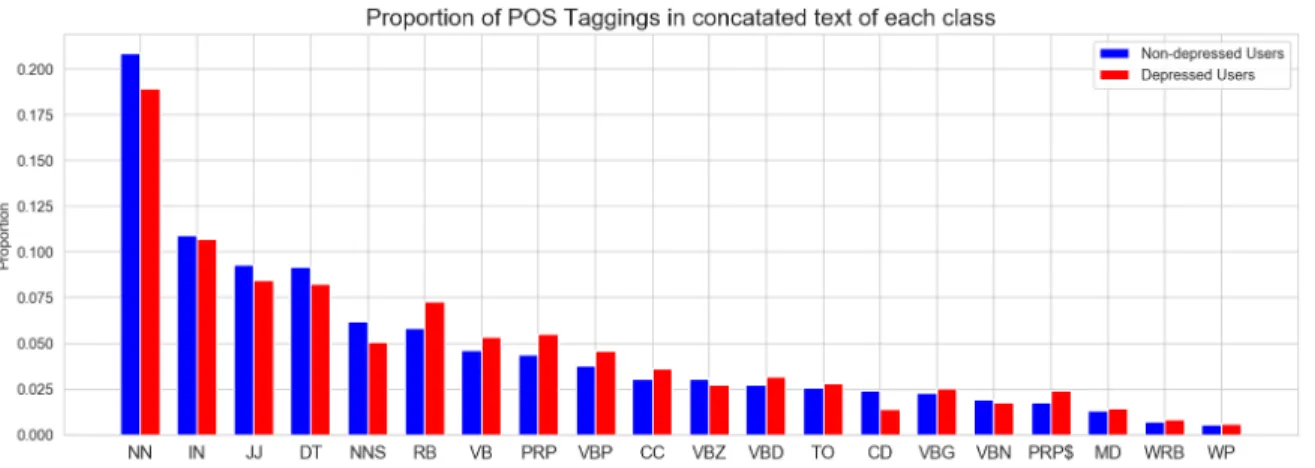
Part-of-speech refers to a group of words with the same function in sentences. The study of Morales and Levitan (2016) indicated that part-of-speech (POS) is an effective indicator for detection of depression. Using the “clean sentences” corpus, I plotted the top 20 POS tagging with the highest proportion among tokens of concatenated text of both depression group and control group in Figure 3 (POS abbreviations can be found in Appendix A). The text used were not lemmatized and all stopwords were kept. TextBlob5
library was used to label each token with part-of-speech. TextBlob is a Python library able to complete simple NLP tasks such as part-of-speech tagging and polarity scoring.
Following the study of Smirnova et al. (2018) which mentioned that depressed individuals showed increased usage of verbs in continuous/imperfective and past tenses as well as personal and indefinite pronouns, I mainly focused on the differences of usage in pronouns and verbs. Figure 3 shows that the depression group shows a higher
proportion among tokens of concatenated text verbs in adverb (RB), verb(VB), present tense(VBP), verbs in past tense (VBD), personal pronouns (PRP) and possessive
pronouns (PRP$). Although it appears that depressed and non-depressed users differed in POS usage, further exploration about POS usage difference need to be conducted in the LIWC (POS categories in the lexicon) feature selection part to determine whether it is a useful feature for classification.
Figure 3: Proportion of top 20 most frequent part-of-speech tagging
4.2.3 Word Proportion
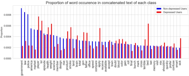
top 50 most frequent tokens among concatenated text for depressed and non-depressed users. The most common and the most rare words were removed before extracting the top 50 words through filter_extremes (no_below=5, no_above=0.5) using the dictionary module of gensim6 . The parameters were set to filter out tokens appearing in less than 5
and no more than 50% concatenated text of users. This parameter setting was chosen because it was it was used by many other researchers and could be adopted for this initial visualization. Figure 4 shows increased usage of words such as “prayer”,
“lol”, ”health”, ”weight”, ”product”, “smoke”, “gon”, ”father”, “apply“, “terrible”, “bed”, “sick” and lower proportion of words such as “government”, “law”, among depressed users.
Figure 4: Proportion of top 50 most frequent words
4.3 Feature Selection
After preprocessing, the data was in the right format for analysis. Extracted features included structural features, topic modeling vectors, polarity scores, inverse document frequency (TF-IDF), count vectorizer, LIWC features and lexical features. I
divided the original training set (see page 16) into a new training set and validation set without changing the distribution of depressed and non-depressed users7. Then TF-IDF,
count vectorizer, lexical features were trained with the new training set and tested on the validation set. Topic modeling features should show meaningful topics and significant different topic distribution among depressed and non-depressed users. Other features (structural features, LIWC features, polarity scores) should have high correlation with the output class (depressed or non-depressed) and low correlation with other features.
Correlation is a statistical concept measuring how likely two variables are linearly
dependent, correlation coefficients between independent variables (selected features) and the output class (depressed or non-depressed) were used to select features with high predictive power. A correlation coefficient close to -1 suggests a strong negative correlation, a coefficient close to 1 suggests a strong positive correlation, a correlation close to 0 suggests weak correlation. Here the absolute value of 0.3 was used to select useful features because correlation coefficient below 0.3 is considered to be weak
(Mukaka, 2012). One assumption under multiple regression models is that all explanatory variables should be independent or it will cause the problem of multicollinearity.
Multicollinearity will undermine the statistical significance of the exploratory variables. To avoid this problem, after features with relatively high correlation with output class (depressed or non-depressed) were selected, a correlation heatmap was drawn to check correlation between those variables.
Features not suitable for correlation calculation such as word2vec vectors were visualized with t-Distributed Stochastic Neighbor Embedding (t-SNE) proposed by
Maaten & Hinton (2006). T-SNE is a state-of-art unsupervised technique to visualize high-dimensional data. It can project high dimensional data to 2-3 dimensions to show a clear visualization of data clustering.
4.3.1 Structural Features
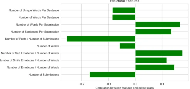
The above exploratory data analysis showed no clear differences in structural features between depressed and non-depressed users. In Figure 5, the correlation
coefficients of structural features proved this observation with the highest absolute value less than 0.3.
Figure 5: Correlation between structural features and output class (depressed or non-depressed)
4.3.2 Topic Modeling
These topics will be assigned to each document based on the probability of co-occurrence of associated words. The probability distribution of topics in each document can be utilized as an input feature for classification tasks. To make topic model vectors as input for the classifier, the following steps were followed. Firstly the topic model was built upon a filtered dictionary (no_above=0.3, no_below=10) with the most common and rare words in the whole corpus removed. This parameter setting was adopted in reference to a topic modeling classifier to detect customer complaints8. I experimented with many topic
numbers but they all did not generate an obvious difference in topic distribution between depressed and non-depressed users. The number of topics was chosen as 50 here because this setting can generate relatively fewer “junk topics” (less occurance of the same words in different topics). Topic distribution was obtained for each class and can possibly act as input for classifiers. Table 5 shows the five most significant words associated with the five most frequent topics for each class. The generated topics don’t make much sense because different topics shared the same words such as “republican”. Besides, depressed and non-depressed users didn’t show significantly different distribution of topics, sharing the most frequent topic 24 and topic 49.
Table 5: Top 5 most frequent words in top 5 most frequent topics for each class
depressed users non-depressed users
For topic 0, the top words are: abandon, boyfriend, republican, batman, climate. For topic 6, the top words are: nasa, california, republican, nuclear, climate. For topic 24, the top words are: republican, rabbit, steam, climate, election.
For topic 43, the top words are: submission, peer, submit, reviewed, abandon.
For topic 49, the top words are: overview,
For topic 1, the top words are: nasa, iraq, republican, climate, fighter.
For topic 24, the top words are: republican, rabbit, steam, climate, election.
For topic 25, the top words are: entry, reviewed, peer, journal, overview.
For topic 30, the top words are: batman, cia, nasa, edition, steam.
For topic 49, the top words are: overview, climate, submit, steam, sander.
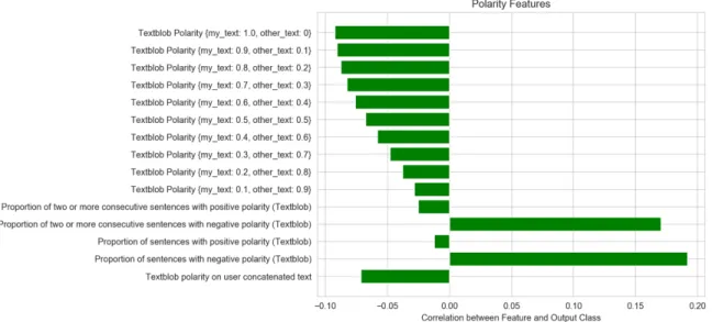
4.3.3 Polarity
Polarity refers to the sentiment of text, namely positive or negative. TextBlob sentiment function was used to obtain polarity scores. It returns polarity scores between -1.0 and -1.0. Scores below 0 stands for negative sentiment and scores above 0 stands for positive sentiment. For example, the polarity score of the sentence “The food was good.” is 0.7, meaning that this sentence is positive. Textblob calculated the polarity score using a Naïve Bayes classifier trained on a labeled dataset of movie reviews.
The polarity score for each user was calculated based on “clean sentences” corpus. Because this dataset contains some non-depressed users active on the depression subreddit, the fact that these users posted about the depression experience of their friends or relatives may cause noise to the polarity scoring. One way to mitigate this noise is to group text into “my_text” and “other_text”. “my_text” include the sentences containing first-person singular pronouns “i”,”me”,”my”,”myself” and ”mine”, while “other_text” include the sentences that don't contain those first-person pronouns. To get a full view of which polarity feature is most effective, I conducted sentence-level calculation on “my_text”, “other_text” and the whole concatenated text for each user. Sentence-level calculation of the polarity score means that the polarity score equals to the mean polarity scores of sentences in the “my_text”, “other_text” or the whole concatenated text of that user. This sentence-level polarity score was named “average sentence polarity”.
“average sentence polarity” of “my_text” and “other_text”. I set the total weight of “my_text” and “other_text” to 1 and the step of weight to be 0.1. The weight ranged from {my_text: 1.0, other_text: 0} to {my_text: 0, other_text: 1.0}. For example, {my_text: 0.9, other_text: 0.1} means that the weight of “my_text” is 0.9 and the weight of
“other_text” is 0.1. These weighted polarity scores were shown in Figure 7 in the form of “Textblob Polarity {my_text: 0.9, other_text: 0.1}”. The second method was to calculate the proportion of positive/negative sentences among all sentences of the concatenated text of each user. This measures how often a user demonstrated positive/negative polarity on a sentence level. It was shown in Figure 7 as “Proportion of sentences with positive polarity (Textblob)” and “Proportion of sentences with negative polarity (Textblob)”. The third method was to compute the proportion of two or more consecutive positive/negative sentences among all sentences of the concatenated text of each user. This measures how often a user demonstrated continuous positive/negative polarity on a sentence level. It was shown in Figure 7 as “Proportion of two or more consecutive sentences with positive polarity (Textblob)”, and “Proportion of two or more consecutive sentences with negative polarity (Textblob)”. The fourth method was to compute the polarity score of “average sentence polarity” of the concatenated text of each user. It was shown in Figure 7 as “Textblob polarity on user concatenated text “.
Figure 6 shows that with “Proportion of sentences with negative polarity
(Textblob)” ranked as the most correlated feature among all polarity scores, and the more weight on “my_text”, the more correlated the features are with the output class
Figure 6: Correlation between polarity features and output class (depressed or non-depressed)
4.3.4 TF-IDF and Count Vectorizer
Both TF-IDF and count vectorizer are based on the bag-of-words (BOW) model. The BOW model focuses on the term frequencies in a given corpus without considering word order. TF-IDF stands for term frequency–inverse document frequency. It can be computed with the formula: TF-IDF = Term Frequency (TF) * log(Inverse Document Frequency) (IDF). Term frequency measures how frequent a term appears in a certain document while inverse document frequency measures how rare the term is in the whole document corpus. Count vectorizer, same as term frequency, refers to the times a term appears in a document. TF-IDF differs from count vectorizer by focusing on words that appear in a particular document but not very frequently in the whole corpus.
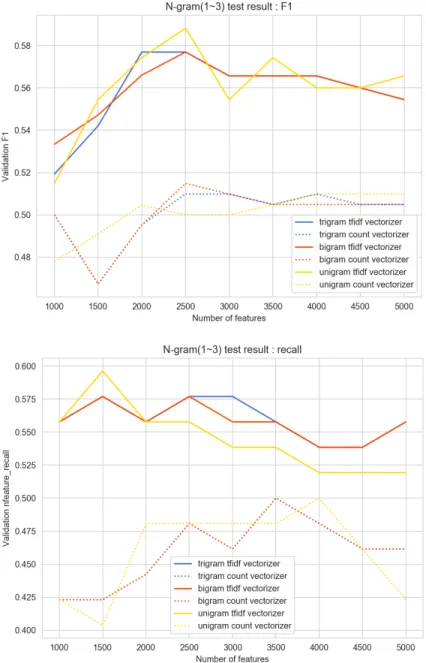
distribution as the original training set. Since the problem of class imbalance exists, here I chose F1 score and recall as evaluation metrics as discussed on page 18. The classifier used for hyper-parameter tuning was logistic regression (LR) classifier, a supervised machine learning technique for classification tasks. After trying with different parameter setting in pilot experiments, I found the when the number of features for this dataset was between 1000 and 5000, the “max_features” (number of features with the highest term frequency) was set between 1000 and 5000, with 500 as the step. The “ngram_range” was set to unigram(1,1), bigram(1,2) and trigram(1,3). Other settings remained as default so that only two parameters, “max_features” and “ngram_range” need to be tuned.
As shown in Figure 7, TF-IDF yielded better performances than count vectorizer with all parameter settings in terms of F1 score and recall. The recall performances of bigram and trigram count vectorizer overlapped with all parameter settings. Among all the parameter settings, when “max_features” was set to 2500, unigram, bigram and trigram TF-IDF generated the highest F1 score with LR classifier. When
4.3.5 Phrase Modeling and Word2Vec
Word2Vec was proposed by Mikolov et al. (2013). In contrast to the BOW model, Word2Vec model aims to learn from the context of words rather than only from the term frequencies. The basis of the Word2Vec model is the distributional hypothesis proposed by Harris (1954), stating that the same context of words means the similar word
meanings. There are two neural network algorithms in the Word2Vec model. One is a continuous bag of words (CBOW), the other is skip-gram. CBOW tries to predict the probability of the word occurrence based on a specific context, while skip-gram tries to predict the probability of corpus words appearing in the context of a specific word. Premchander et al. (2018) stated that CBOW is used for smaller dataset. The Word2Vec mode was built upon “tokenized sentences” corpus and the number of sentences in the training set was 529,614, so I chose skip-gram model as the algorithm for the Word2Vec model. To compare the performance of Word2Vec embeddings with unigram and bigram detected, the Phraser model in Gensim was applied to build a bigram model with all concatenated text in the training set. Then the “unigram tokenized sentences” corpus was transform to “bigram tokenized sentences” corpus.
The training results on different corpus sets were surprising. Since ski-gram model of Word2Vec learns from word context (neighboring words), stopwords can provide more dependency information. However, Table 6 shows that by removing the stopwords, word vectors generated better performance for both unigram and bigram corpus sets. This could be due to the fact that some sentences contain only a few tokens, but many stopwords such as “a”, “the” were not very useful when dealing with these shorter sentence corpus. Another finding was that bigram corpus set achieved a higher F1 score than unigram corpus set with or without removing stopwords. Furthermore,
the best F1 score and an acceptable recall score. The t-SNE (Figure 8) showed that by using Word2Vec vectors trained on “bigram tokenized sentences” corpus where sentence lengths are larger than 2, it generated two clear clusters of users. However, because the performance levels of “bigram tokenized sentences” corpus with and without stopwords were very close, neither of them was chosen or rejected and remained to be compared when combined with other features discussed in the following sections.
Table 6: Performance of Word2Vec trained on different corpus
Corpus Set F1 Recall
unigram tokenized sentences 0.5131 0.7500
unigram tokenized sentences with stopwords 0.5055 0.8846
bigram tokenized sentences 0.5306 0.7500
bigram tokenized sentences where sentence lengths are larger than 2 tokens
0.5369 0.7692
bigram tokenized sentences with stopwords 0.5056 0.8654
bigram tokenized sentences with stopwords where sentence
4.3.6 LIWC Features
Losada and Crestani (2016) didn’t document that all text in the dataset was written in English, but because the depressed users were collected by identifying English diagnosis statements “I was diagnosed with depression” and Reddit is primarily written in English9, I assumed that all text in this dataset was written in English. Depression can
lead to different language patterns and here I only focused on English speakers. Smirnova et al. (2018) mentioned that more verbs in continuous/imperfective (e.g., have been thinking) and past tenses (e.g., thought) were used among depressed individuals
compared with healthy individuals. The increased usage of past tense words indicated a
9https://en.wikipedia.org/wiki/Reddit
tendency of rumination among depressed people. Brockmeyer et al. (2015) also noticed that elevated usage of first person pronouns { “i”, “me”, “my”, “myself”, “mine”} came with symptoms of depression. The reason behind it could be that singular first-person pronouns suggest more self-focused attention. Moreover, absolutist words such as “definitely” and “always” are more common in the depression group. People affected by depression are more likely to think in an all-or-nothing way (Al-Mosaiwi & Johnstone, 2018).
Linguistic Inquiry Word Count (LIWC), a text analysis program counting
occurrences of words or stems for 64 pre-defined psychometric categories in a given text (Pennebaker et al., 2007). Each word found in a given text belongs to one or more categories. For example, the word “thought” is part of categories of verbs, past tense, cognitive process and insight. As discussed in the last paragraph, linguistic features of depressed users included increased usage of first-person pronouns, verbs in past and continuous/imperfective tense, etc. While most of these linguistic features were included in LIWC categories, I defined a list of absolutist words according to an online resource10
to be a supplement to LIWC features. The proportions of words in 64 pre-defined LIWC categories and absolutist words in concatenated text of each user were treated as a feature. Figure 9 shows the LIWC categories whose correlation with the output class (depressed or non-depressed users) is higher than the 0.3 threshold as defined on page 28. The problem of multicollinearity, which means excessive correlation between two
predictors/features or between one predictor/feature and linear combination of the predictors/features, should be avoided because it can cause a problem to generalized
Figure 10: Correlation between selected LIWC features (correlation with output class is above 0.3) and output class (depressed or non-depressed)
4.3.7 Lexical Features
Apart from the word vector features, lexical features were also considered helpful in sentiment analysis. As Blinov et. al (2013) suggested, I manually built a
corpus-specific emotion dictionary and attached sentiments weights to words. The “sentiment weight” was related to how correlated a word was to the positive class (depressed users). Mutual information between word and class measures how much information the
presence of a word can give to the correct prediction of a class, but it didn’t act as a good predictor when fed into the logistic regression classifier. Inspired by the method of
cumulative distribution function of word frequencies proposed by Moreno, Font-Clos and Corral (2017), I calculated P(positive|word) and P(word|positive).
B(!'&%D%E# | G'"H) = #!'&%D%E# $<;&& '$$J""#($#& #;<< '$$J"#($#&
B(G'"H | !'&%D%E#) = #!'&%D%E# $<;&& '$$J""#($#& #;<< !'&%D%E# G'"H&
P(positive|word) measures how often the positive class appears with the presence of a word, while P(word|positive) measures how often a word appears in the positive class. Then I got the cumulative distribution function (CDF) of these two values. CDF is defined as the probability of a variable X with a value less than or equal to x. The CDF calculation can provide us with information about where a word lies in terms of these two values in a cumulative perspective. For example, CDF(P(positive|”sleep”)) is 0.994591 and P(positive|”sleep”) is 0.375929, which means that the probability of
K = ( ∑(%=1
M%
1
The harmonic means were the final sentiment weights of this manually built dictionary. Each document in the training and validation set were scored with this emotional dictionary. Figure 11 and Figure 12 show the top words ranked by lexical features and evaluation results achieved only by using the lexical features respectively. The words in Figure 11 can represent favored words of depressed users.
RESULTS 5.1 Evaluation
Models were trained on all chunks of training dataset, the tuned models were tested on 0-10 chunks of data. Due to the sensitivity to time in early detection tasks, the metrics of early detection tasks should lay emphasis on both correctness and the
consumed time, which means using the fewest chunks of test data to achieve a relatively high performance. Losada et al. (2017) introduced a metric called Early Risk Detection Error (ERDE) taking into account the delay cost. Assuming that the time of processing each document is the same, instead of the number of distinct textual submissions processed before the classifier making the decision (Losada et al., 2017), the delay in detection was defined as the number (k) of chunks here. To prevent a classifier from always predicting negative, false positive predictions were penalized according to the positive class proportion in the whole data. For example, if ERDE of false negative predictions equals 1, then ERDE of false positive predictions could be the percentage of positive classes in all data. True positive predictions were assigned a delay cost (1
-1/(1+ek-o)), where o controls the value of x-axis where the cost grows dramatically, here o
NO !"#H%$D%'( %& O;<&# !'&%D%E#, QRSQ = # ;<< !'&%D%E# %(&D;($#& # ;<< %(&D;($#&
NO !"#H%$D%'( %& O;<&# (#T;D%E#, QRSQ = 1 NO !"#H%$D%'( %& D"J# !'&%D%E#, QRSQ = H#<;U $'&D NO !"#H%$D%'( %& D"J# (#T;D%E#, QRSQ = 0
5.2 Classifiers
After the feature selection process, the final features were TF-IDF vectors, Word2Vec vectors (trained on “bigram tokenized sentences” corpus with and without stopwords), LIWC features and lexical features. The Word2Vec vectors trained on bigram tokenized sentences without stopwords yielded a better performance when combining with other features, so it was chosen as the final Word2Vec feature. The classifiers I chose were logistic regression (LR) and Linear Support Vector Machine (SVM). The two classifiers performed well in previous research (e.g., Stankevich et al. (2018), Trotzek et al. (2018), De Choudhury et al. (2013, June), Kang, Yoon, and Kim (2016)) about detecting mental disorders via social media. In addition, after initial cross validation on the training set, these two classifiers generated better results than other classifiers (e.g., random forest classifier and adaptive boosting classifier). Table 7 shows the experiment results in the order from a single-feature model to all-feature model for both LR and SVM classifier. LR classifier achieved the highest F1 score 0.6207 when using TF-IDF and Word2Vec and tested on all chunks of test data. Similarly, SVM classifier achieved the highest F1 score 0.5833 when using TF-IDF and Word2Vec tested on all chunks of test data. In experiments with these two classifiers on all test data, LR classifier stood out in nearly all evaluation metrics in terms of F1 and recall, while SVM classifier generated a better precision and modified QRSQ5. The PR curve of classifiers generating the best F1 score
Table 7: Experiment results using different features and classifiers on all test data
Feature Model Accuracy F1 Precision Recall Modified QRSQ5 LR experiment results
TF-IDF LR 0.8878 0.5872 0.5614 0.6154 14.8074
TF-IDF+Word2Vec LR 0.8903 0.6207 0.5625 0.6923 16.4171
TF-IDF+LIWC LR 0.8853 0.5741 0.5536 0.5962 14.5921
TF-IDF+lexical LR 0.8827 0.5766 0.5424 0.6153 15.3062
TF-IDF+Word2Vec+LIWC
LR 0.8903 0.6207 0.5625 0.6923 16.4171
TF-IDF+Word2Vec+lexica l
LR 0.8903 0.6207 0.5625 0.6923 16.4171
TF-IDF+LIWC+lexical LR 0.8778 0.5664 0.5246 0.6154 15.8049
Word2Vec+TF-IDF+LIWC+lexical
LR 0.8878 0.6154 0.5538 0.6923 16.6665
SVM experiment results
TF-IDF SVM 0.8977 0.5684 0.6279 0.5192 11.4861
TF-IDF+Word2Vec SVM 0.9002 0.5833 0.6364 0.5385 11.7015
TF-IDF+LIWC SVM 0.8978 0.5684 0.6279 0.5192 11.4861
TF-IDF+lexical SVM 0.9002 0.5745 0.6429 0.5192 11.2367
TF-IDF+Word2Vec+LIWC
SVM 0.9002 0.5833 0.6364 0.5385 11.7015
TF-IDF+LIWC+lexical SVM 0.9002 0.5745 0.6429 0.5192 11.2367
TF-IDF+Word2Vec+lexica l
SVM 0.9002 0.5833 0.6364 0.5385 11.7015
Word2Vec+TF-IDF+LIWC+lexical
After the initial test on all test data, it appeared that TF-IDF and Word2Vec were the minimum features needed to generate the best F1 score. When tested on all test data (Table 5), LIWC features and lexical features didn’t increase performance of any model. However, they improved the model resilience to the decrease of chunk numbers in pilot experiments on different chunks of test data. Therefore, all four features were kept to be tested on different chunks of test data. Built upon the previous results, LR and SVM classifiers were tested on different chunks of test data in the chronological order to test the model’s ability of early detection (with less chunks of test data as possible).
The test was run 10 times from chunk 1 to chunk 10, with each iteration, an additional chunk of data containing user submissions of a more recent time was added to the test set. The experiment results of LR classifier were shown in Figure 14, Figure 16 and Table 8. The experiment results of SVM classifier are shown in Figure 16, Figure 17 and Table 9.
It is noticeable that the performance of LR classifier increased as the number of chunks increased and it experienced a performance boost from chunk 1 to chunk 6. With
the object to generate high F1 score and low ERDE and given that ERDE increases along with the chunks of test data used, as fewer chunks of test data as possible should be used to generate a good F1 score. The least number of chunks LR classifier needs to generate a relatively good F1 score is 6.
All metrics of SVM classifier only experienced mild changes after 6 chunks of test data, taking ERDE metric into account, the least number of chunks the classifier needs to generate both high F1 and ERDE score is also 6.
Figure 15: Accuracy, F1, precision, recall of SVM classifier
Figure 16: Modified ERDE of LR classifier Figure 17: Modified ERDE of SVM classifier
Table 8: Experiment results using logistic regression
#Chunk Accuracy F1 Precision Recall Modified QRSQ5
1 0.8728 0.4356 0.4490 0.4231 7.7168
2 0.8853 0.4753 0.4898 0.4615 7.9664
3 0.8778 0.4529 0.4444 0.4615 8.5750
4 0.8628 0.4660 0.4705 0.4615 9.8446
5 0.8803 0.5472 0.5370 0.5577 11.8037
6 0.8803 0.5932 0.5303 0.6731 13.7628
7 0.8853 0.6034 0.5467 0.6731 15.0324
8 0.8828 0.5841 0.5410 0.6347 15.6410
9 0.8828 0.5913 0.5397 0.6538 15.8906
10 0.8878 0.6154 0.5538 0.6923 15.9863
Table 9: Experiment results using support vector machine
#Chunk Accuracy F1 Precision Recall Modified QRSQ5
1 0.8703 0.3500 0.5000 0.2692 7.9105
2 0.8852 0.4390 0.6000 0.3462 8.1748
3 0.8803 0.4286 0.5625 0.3462 8.8192
4 0.8953 0.5000 0.6563 0.4038 10.1635
5 0.8928 0.4941 0.6364 0.4038 12.2378
6 0.8953 0.5435 0.6250 0.4807 14.3121
7 0.8953 0.5333 0.6316 0.4615 15.6564
8 0.8953 0.5435 0.6250 0.4808 16.3008
9 0.8853 0.5208 0.5682 0.4808 16.5651
DISCUSSION
This study aims to detect depressed users on Reddit using the CLEF/eRisk 2017 dataset (Losada et al.2017). TF-IDF, Word2Vec, LIWC features, and lexical features based on a sentiment dictionary were chosen as the most effective features for this classification task. When using these four features alone with LR classifier, TF-IDF generated a F1 score of 0.5825 on its own. Although Word2Vec didn’t generate a better result than TF-IDF, it did boost the F1 score when combined with TF-IDF to 0.6207. It is also noted that with bigram phrase modeling, the Word2Vec vectors yielded a much better F1 score. Based on previous research about language patterns of people with depression (Smirnova et al. (2018), Brockmeyer et al. (2015)), I assumed that linguistic characteristics such as increased usage of verbs in past tense, first-person singular
pronouns, absolutist words, affective words and health related words can contribute to the classification task. These characteristics transformed into features using the proportion of words in 64 LIWC categories and an additional absolutist word list. Among all LIWC combined with absolutist word features had many dimensions, “first person
singular”, ”sadness”, “health” showed a higher correlation with the output class
(depressed or non-depressed) than the rest of the features. For lexical features, I manually built a bigram sentiment dictionary using concatenated text of all training set users and assigned weights to each word with the harmonic mean of P(positive|word) and
resulting in a F1 score 0f 0.54. Although LIWC and lexical features didn't increase the classifier performance when tested on all test data, they improved the model resilience to the decrease of the number of chunks of test data.
Features failing to perform well in this classification task also provide insights into future work. All structural features showed smaller than 0.3 correlation with the output class(depressed or non-depressed users), The proportion of posts (initiated
CONCLUSION
This thesis explored various features and approaches to better detect depressed users via Reddit posts containing textual data. By combining the basic natural language technique TF-IDF and the state-of-art Word2Vec model trained on “bigram tokenized sentences” with stopwords removed, LR classifier achieved the best F1 score of 0.6207 when tested on whole test data. When tested on different chunks of test data to achieve a low ERDE and high F1 score, LIWC features and sentiment dictionary features were combined with TF-IDF and Word2Vec in the purpose of increasing the model resilience to fewer chunks of test data. Given that ERDE increases along with the chunks of test data used, the least number of chunks LR classifier needs to generate a relatively good F1 score (0.5932) is 6. It need further development to be put into use for preliminary
screening of depression, general learnings and future works are presented in the following paragraphs.
(depressed or non-depressed) than the rest of the LIWC features. In addition to LIWC features, chi-squared statistics suggested additional types of words that differentiated the two output class. Here I grouped these words into five categories. The first one includes relationship words: “relationship”, “boyfriend”, “girl” , “friend”, “mom”, “parent”, “baby”. The second one includes medical words: “doctor”. The third one includes physical feelings: ”pain”, ”sleep”, “skin”. The fourth one includes emotional feelings: “anxiety”, ”depression”, ”happy”, ”feel”, ”feel_like”. The fifth one includes absolutist words: “definitely”.
Compared with other participants in the CLEF/eRisk 2017 test, the best F1 score (0.6207) in this study achieved in this study was better than some participants in the CLEF/eRisk 2017 task (see Appendix B), but didn’t perform as well as other participants (Trotzek et al., (2018), Stankevich et al. (2018)). One reason may be that the models achieving higher F1 score might be that it used manually built features and word vectors rather than the established word embeddings directly. For example, Trotzek et al. (2018) used user-based metadata features including “month of writings” and occurrences of special phrases such as “therapist”, while my models only utilized textual features and didn’t include domain specific phrase extraction. Furthermore, other word embeddings such as GloVe1 may contribute to a better performance (Stankevich et al., 2018).