INTEGRATING ENGINEERED WETLANDS WITH CROP IRRIGATION: AN EVALUATION OF CHEMICAL UPTAKE
Ramón DC Alatorre
A thesis submitted to the faculty of the University of North Carolina at Chapel Hill in partial fulfillment of the requirements for the degree of Masters of Science in the Department of
Environmental Sciences and Engineering.
Chapel Hill 2012
Approved by:
ii
ABSTRACT
RAMÓN DC ALATORRE: Integrating Engineered Wetlands with Crop Irrigation: An Evaluation of Chemical Uptake
(Under the direction of Dr. Howard Weinberg)
iii
ACKNOWLEDGEMENTS
I would like to thank my family for their constant support and for always encouraging my education. I am especially grateful to my adviser, Dr. Howard Weinberg, for constantly promoting my personal and professional growth, as well as my research while at UNC. I would like to thank Dr. Halford House and Dr. Steve Whalen for serving on my committee and reading my thesis. Additionally I would like to thank Dr. Owen Duckworth and Dr. Steve Broome from North Carolina State University for providing valuable input and
resources to pursue the project. I am appreciative of Fernando Rubio and Dave Deardorff of Abraxis Kits LLC for providing training, materials, and support in the use of ELISA kits. I am grateful for the financial support from The National Science Foundation Alliances for Graduate Education and the Professoriate (AGEP) as well as the Department of
iv
TABLE OF CONTENTS
LIST OF TABLES ... xiii
LIST OF FIGURES ... xx
LIST OF SYMBOLS AND ABBREVIATIONS ... xxiv
CHAPTER 1: BACKGROUND INTRODUCTION AND LITERATURE REVIEW ... 2
1.1 Anthropogenic Influence on Water Sources ... 2
1.1.1 PPCPs & EDCs: Their Presence in the Environment and Their Repercussions ... 2
1.2 Water Reclamation and Reuse: A “Keeping the Horse Before the Cart” Solution ... 4
1.3 Additional Benefits Attributable to Water Reclamation and Reuse ... 5
1.3.1 Water Quantity: Primary and Secondary Benefits ... 5
1.3.2 Economic Benefits ... 7
1.3.2.1 Green Infrastructure and the Green Economy ... 8
1.3.3 Developing World Applications... 8
1.3.4 Water Reclamation and Irrigation: Proceed with Caution? ... 9
1.4 Crop Analysis... 10
1.4.1 Presence of Anthropogenic Chemicals Including PPCPs and EDCs in Plants ... 10
1.4.2 Techniques ... 11
1.4.2.1 ELISAs vs. Chromatography: Speed vs. Multiresidue Analysis ... 12
1.4.3 Benefits of Thinking Faster/Cheaper: Screening and Public Health... 13
v
1.4.3.2 QuEChERS + ELISAs: Screening Match Made in Heaven? ... 15
1.4.4 Chemical Indicators... 16
1.4.4.1 Proposed Indicator: Caffeine ... 17
1.4.4.2 Proposed Indicator: Triclosan ... 17
1.4.4.3 Proposed Indicator: Estradiol ... 18
1.4.5 Potential for Crop Uptake and Translocation ... 18
1.4.6 Summary of Proposed Indicators for Crop Uptake of Waste Water Contaminants ... 22
1.5 Objectives of the Research ... 22
CHAPTER 2: EXPERIMENTAL SKETCH, MATERIAL AND METHODS ... 26
2.1 Field Study Experimental Sketch... 26
2.1.1 The Two Crops ... 26
2.1.2 The Three Waters ... 25
2.1.3 The Two Growing Matrices ... 25
2.2 Materials ... 26
2.2.1 Laboratory Materials ... 26
2.2.1.1 Chemicals ... 26
2.2.1.2 Other Laboratory Materials Used ... 27
2.2.1.3 Cleaning Procedures ... 29
2.2.2 Field Materials... 29
2.3 Site Descriptions ... 31
2.3.1 Source of Reclaimed Waste Water: Jordan Lake Business Center on-site Integrated Water Strategies (IWS) Water Reclamation System in Chatham County, NC ... 31
vi
2.3.2.1 Physical Layout and Treatment Group Blocking ... 33
2.3.2.2 Reservoir Storage ... 34
2.3.2.3 Automated Irrigation System ... 34
2.4 Field Methods ... 37
2.4.1 Collection of Water from Field Site ... 37
2.4.2 Filling the Reservoirs ... 37
2.4.3 Collecting Water Samples from Reservoirs ... 38
2.4.4 Covington Sweet Potatoes: Planting, Irrigation Summary and Harvest ... 38
2.4.5 Parris Island Lettuce: Planting, Irrigation Summary and Harvest ... 39
2.5 Laboratory Methods ... 39
2.5.1 Homogenization and Sample Preparation for Extraction:... 39
2.5.1.1 Sweet Potatoes ... 39
2.5.1.2 Sweet Potato Leaves ... 41
2.5.1.3 Lettuce Leaves ... 42
2.5.1.4 Sand and Soil Samples ... 43
2.5.2 Sample Extractions, Fractions, Concentration and Storage ... 43
2.5.2.1 Sweet Potatoes ... 45
2.5.2.2 Sweet Potato and Lettuce Leaves ... 48
2.5.2.3 Sand/Soil ... 48
2.5.3 Analytical Instrumentation, Software and the Abraxis Enzyme Linked Immunosorbent Assay (ELISA) kits:... 49
2.5.3.1 Gas Chromatography ... 49
2.5.3.1.1 Ion Trap Mass Spectrometry ... 49
vii
2.5.3.2 Abraxis Enzyme Linked Immunosorbent Assay (ELISA) Method ... 51
2.5.3.3 Additional Software ... 52
2.6 Supplemental Methods Section... 52
2.6.1 Glassware Silinization Method: Used to prepare conical vials prior to derivatization ... 52
2.6.2 Derivatization Method A ... 53
2.6.3 Derivatization Method B: Acetonitrile Reconstitution ... 53
CHAPTER 3: RESULTS AND DISCUSSION ... 55
3.1 Method Compatibility and Extraction Efficiency ... 55
3.1.1 Strategies Utilized ... 55
3.2 A Chronological Evolution Investigating Method Compatibility ... 57
3.2.1 Phase 1 Investigation: Grocery Store Sweet Potato Tissue... 57
3.2.1.1 ELISA Analysis of Grocery Store Sweet Potato Extracts ... 58
3.2.1.2 GC-ECD Analysis of Grocery Store Sweet Potato Extracts ... 63
3.2.1.3 Ion Trap GC-MS Analysis of Grocery Store Sweet Potato Extracts ... 64
3.2.1.4 Conclusions of Initial Analysis of Grocery Sweet Potato Extracts ... 69
3.2.2 Phase 2 Investigation: Analysis of Extracts of Sweet Potato Leaf Tissue from an Agricultural Field Site ... 69
3.2.2.1 Standard Addition: Caffeine Analysis ... 71
3.2.2.2 Standard Addition: Triclosan Analysis ... 72
3.2.2.3 Standard Addition: Estradiol Analysis ... 73
3.2.2.4 Homogenate Spike Recovery from Sweet Potato Leaves ... 73
viii
3.2.3 Phase 3: Analysis of All Greenhouse Experimental Matrices Near
Environmental Concentrations ... 77
3.2.3.1 Sample Preparation and Extraction ... 78
3.2.3.2 Analysis of Working Solution #5 ... 80
3.2.3.3 Caffeine ELISA Compatibility and Recovery Analysis of QuEChERS Crop and Soil Extracts ... 81
Standard Addition Compatibility Analysis ... 81
Homogenate Spike Recovery Analysis ... 83
Unspiked Homogenate Extract Analysis... 84
3.2.3.4 Triclosan ELISA Compatibility and Recovery Analysis of QuEChERS Crop and Soil Extracts ... 85
Standard Addition Compatibility Analysis ... 85
Homogenate Spike Recovery Analysis ... 86
Unspiked Homogenate Extract Analysis... 87
3.2.3.5 Estradiol ELISA Compatibility and Recovery Analysis of QuEChERS Crop and Soil Extracts ... 88
Sweet Potato Tissue and Lettuce Leaf Tissue ... 88
Sand and Soil ... 89
3.3 Implications of Method Compatibility Investigations for the Analysis of Greenhouse Irrigated Samples: ... 90
3.3.1 Estradiol ... 90
3.3.2 Caffeine and Triclosan ... 91
Sweet Potato Tissue ... 91
Lettuce Leaves ... 91
Sweet Potato Leaves ... 92
ix
Soil ... 93
3.4 Analysis of Greenhouse Samples... 93
3.4.1 Reservoir Analysis ... 93
3.4.2 Crop Tissue and Growing Matrices Analysis ... 94
3.4.2.1 Fall 2011 Trend and “Concentration” Approach ... 95
3.4.2.2 Spring 2012 Trend Approach ... 97
3.5 Fate and Transport of Caffeine ... 98
3.5.1 Fall 2011 Trend and “Concentration” Analysis: Caffeine ... 98
3.5.1.1 November 28, 2011 ... 98
3.5.1.2 November 29, 2011 ... 100
3.5.1.3 December 23, 2011 ... 101
3.5.2 Spring 2012 Trend and Concentration Analysis ... 102
3.6 Fate and transport of triclosan ... 105
3.6.1 Fall Trend and “Concentration” Analysis: Triclosan ... 105
3.6.1.1 November 28, 2011 ... 105
3.6.1.2 November 29, 2011 ... 106
3.6.1.3 December 23, 2011 ... 107
3.6.2 Spring 2012 Trend and Concentration Analysis: Triclosan ... 108
Sand and Soil ... 108
Sweet Potato Tissue ... 109
Sweet Potato Leaves ... 110
x
3.7 Fate and Transport of Estradiol ... 111
Crop Tissues ... 111
Sand and Soil ... 111
CHAPTER 4: CONCLUSIONS AND RECOMMENDATIONS ... 113
4.1 Method Compatibility ... 113
4.2 Fate and Transport ... 117
Caffeine ... 117
Triclosan ... 119
Estradiol ... 120
4.3 Final Comments ... 121
APPENDIX A: STOCK AND WORKING SOLUTIONS ... 122
A.1 Stock solutions in acetonitrile (used to make working solutions) ... 122
A.2 Working solutions used for Phase 1 investigation ... 123
A.3 Working solutions for Phase 2 investigation ... 124
A.4 Working solution #5 for Phase 3 analysis ... 125
A.5 Working solutions in acetonitrile for homogenate-spikes and spikes into QuEChERS extracts of greenhouse samples ... 126
APPENDIX B: PHASE 1 INVESTIGATION ... 127
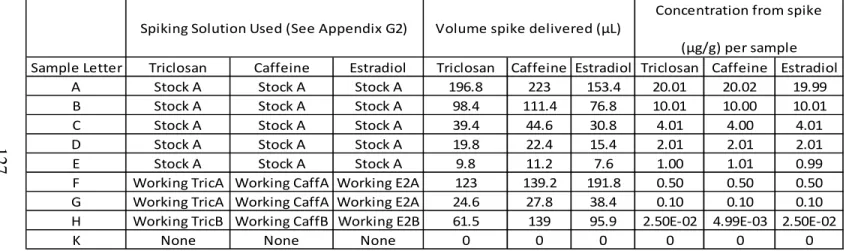
B.1 Phase 1 investigation; execution of spikes onto sweet potato homogenates... 127
B.2 Phase 1 investigation; ELISA responses and recovery of target compounds spiked onto sweet potato homogenates ... 128
B.3 Phase 1 investigation; GC-ECD retention time and peak area response to QuEChERS extracts of sweet potato, homogenates spiked with known masses of triclosan ... 130
xi
B.5 Phase 1 investigation; GC-Ion-Trap-MS signal to noise responses to neat standards of target compounds and determination of instrument
detection limits (IDL) ... 132 B.6 Phase 1 investigation; GC-Ion-Trap-MS signal to noise responses to
homogenate spiked sweet potato samples and determination of practical
detection limits (PDL)... 133 APPENDIX C: PHASE 2 INVESTIGATION ... 139 C.1 Phase 2 investigation; homogenate and extract preparation and execution ... 139 C.2 Phase 2 investigation; ELISA responses to standard addition spikes into
unspiked homogenate extract (no-dSPE) ... 140 C.3 Phase 2 Investigation ELISA responses and recovery of homogenate spiked
extracts with dSPE cleanup ... 141 C.4 Phase 2 investigation; ELISA responses and recovery of homogenate spiked
extracts without dSPE cleanup... 142 C.5 Phase 2 investigation; determining the impact of dSPE on ELISA response ... 144 APPENDIX D: PHASE 3 INVESTIGATION ... 149 D.1 Phase 3 investigation; sample designation, preparation, and execution of
extractions from matrices ... 149 D.2 Phase 3 investigation; extract dilutions and designations for ELISA analysis ... 150 D.3 Phase 3 investigation; ELISA analysis of working solution #5 used to spike
onto homogenates and into finished extracts ... 152 D.4 Phase 3 investigation; caffeine ELISA analysis of extract-spiked samples
and unspiked homogenate extracts ... 154 D.5 Phase 3 investigation; Triclosan ELISA analysis of extract-spiked samples
and unspiked homogenate extracts ... 157 D.6 Phase 3 investigation; estradiol ELISA analysis of extract-spiked samples
xii
D.9 Phase 3 investigation; estradiol ELISA homogenate spike-recovery analysis ... 169
D.10 Phase 3 investigation; caffeine ELISA analysis of stored extracts ... 171
D.11 Phase 3 investigation; triclosan ELISA analysis of stored extracts ... 172
D.12 Phase 3 investigation; estradiol ELISA analysis of stored extracts ... 173
APPENDIX E: ANALYSIS OF RESERVOIRS ... 174
xiii
LIST OF TABLES
Table 1: Relevant Chemical Properties of Proposed Indicators ... 17 Table 2: Full workup of the 7 homogenates into the 9 final treatment extracts
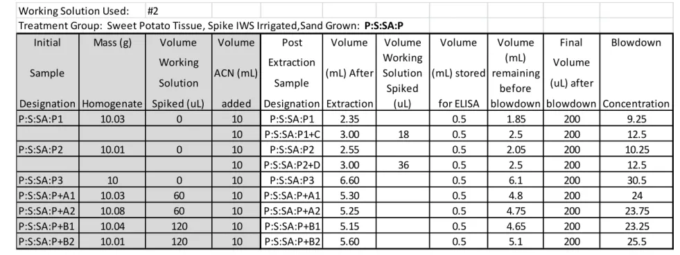
for of the treatment group P:S:SA:P ... 47 Table 3: Working solution #2 and the resulting spike boost to the A,B,C,D
samples of P:S:SA:P ... 47 Table 4: Concentration (µg/g) of spikes delivered onto sweet potato homogenates ... 57 Table 5: Quantitation ranges for each ELISA kit investigated ... 58 Table 6: Interpolated concentration of triclosan standards based on their
response on the calibration curve with upper and lower bounds for the
99% Confidence Intervals (CI). ... 59 Table 7: ELISA response to extracted grocery store sweet potato homogenates
for triclosan ... 60 Table 8: GC-Ion Trap-MS responses and apparent Instrument Detection Limit
(IDL) to neat solutions of caffeine and triclosan in acetonitrile and
derivatized estradiol in hexane... 66 Table 9: GC-Ion Trap-MS responses to filtered acetonitrile QuEChERS extracts
of sweet potato and derivatized extracts with apparent Practical Detection
Limit (PDL) reported for each target compound ... 67 Table 10: Phase 2 sample designations and concentration of compounds spiked
onto homogenates. ... 70 Table 11: Standard addition spikes delivered into the extract of unspiked-leaf
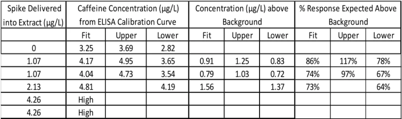
homogenate (Sample 1) ... 71 Table 12: ELISA responses for caffeine in spiked extracts of sweet potato leaves
processed without dSPE ... 72 Table 13: ELISA analysis of caffeine spiked sweet potato leaf homogenates with dSPE .... 73 Table 14: ELISA analysis of caffeine spiked sweet potato leaf homogenates
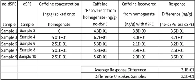
without dSPE. ... 74 Table 15: Determining the difference in caffeine ELISA response for extracts
xiv
Table 16: Homogenate masses, volume of working solution spiked onto homogenates, and volume of acetonitrile used to perform each
Phase 3 extraction ... 79 Table 17: ELISA analysis of caffeine in Working Solution #5 ... 81 Table 18: Caffeine ELISA analysis of extract-spiked and unspiked homogenate
extracts of sweet potato tissue (P:G:SO:P) compared to expected
responses from spike delivered ... 82 Table 19: Spike recovery analysis and concentration of caffeine within sweet
potato tissue irrigate with tap water (P:G:SO:P). ... 84 Table 20: Triclosan ELISA analysis of extract-spiked and unspiked homogenate
extracts of sweet potato tissue (P:G:SO:P) compared to expected
responses from spike delivered ... 85 Table 21: Spike recovery analysis and concentration of triclosan within sweet
potato tissue irrigate with tap water (P:G:SO:P)... 87 Table 22: Estradiol ELISA analysis of extract-spiked sweet potato homogenate
extracts and unspiked-homogenate extracts. ... 88 Table 23: Estradiol ELISA analysis of extract-spiked lettuce leaf homogenate
extracts and unspiked-homogenate extracts. ... 88 Table 24: Estradiol ELISA analysis of extract-spiked soil homogenate extracts
and unspiked-homogenate extracts ... 90 Table 25: Estimated mass of target analytes delivered to sweet potato and lettuce
based on limited reservoir analysis (Appendix E) and volume applied... 94 Table 26: Coding used to identify sample extracts from the greenhouse experiments. ... 98 Table 27: Fall 2011 ELISA trend and “concentration” analysis of caffeine
within greenhouse grown sweet potato tissues and growing matrices. ... 99 Table 28: Spring 2012 ELISA trend and concentration analysis of caffeine within
greenhouse grown sweet potato tissue, lettuce leaves, and soil ... 103 Table 29: Fall 2011 ELISA trend and “concentration” analysis of triclosan within
greenhouse grown sweet potato tissues and growing matrices. ... 105 Table 30: Spring 2012 ELISA trend and concentration analysis of triclosan within
xv
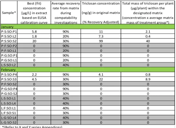
Table 31: Spring 2012 ELISA trend and concentration analysis of triclosan within greenhouse grown sweet potato tissues, lettuce leaves, and growing
matrices (Continued) ... 110
Table 32: Spring 2012 ELISA trend and concentration analysis of estradiol within greenhouse irrigated growing matrices ... 112
Table 33: Practical Detection Limits for GC-Ion-Trap-MS ... 113
Table 34: Potential Detection Limits of ELISA kits ... 114
Table 35: Caffeine ELISA analysis of extract-spiked and unspiked homogenate extracts of virgin (non-irrigated) soil (VSO) compared to expected r esponses from spike delivered ... 115
Table 36: Stock solutions (Batch "A") of target compounds in acetonitrile ... 122
Table 37: Stock solutions (Batch "B") in acetonitrile ... 122
Table 38: Phase 1 working solutions in acetonitrile (used to spike onto homogenates) ... 123
Table 39: Phase 1 GC-MS neat solution "Mix A" in acetonitrile ... 123
Table 40: Derivatized neat samples (using derivatization method A) in silinized glassware ... 123
Table 41: Phase 2 working solutions for spiking onto homogenates of sweet potato leaf .. 124
Table 42: Phase 2 working solutions for spiking into QuEChERS extracts of sweet potato leaf ... 124
Table 43: Working solution (#5) for delivering homogenate-spikes and spikes into QuEChERS extracts of Phase 3 Investigation ... 125
Table 44: Greenhouse samples extraction working solution (#1) for delivering homogenate-spikes and spikes into QuEChERS extracts ... 126
Table 45: Greenhouse samples extraction working solution (#2) for delivering homogenate-spikes and spikes into QuEChERS extracts ... 126
Table 46: Greenhouse samples extraction working solution (#3) for delivering homogenate-spikes and spikes into QuEChERS extracts ... 126
xvi
Table 48: Execution of homogenate spikes onto sweet potato homogenate
and concentration of samples created ... 127 Table 49: Caffeine ELISA responses and recovery of spikes onto grocery store
sweet potato homogenates ... 128 Table 50: Triclosan ELISA responses and recovery of spikes onto grocery store
sweet potato homogenates ... 128 Table 51: Estradiol ELISA responses and recovery of spikes onto grocery store
sweet potato homogenates ... 129 Table 52: Triclosan spike delivered (µg/g) onto homogenates of sweet potato samples .... 130 Table 53: GC-ECD retention time and peak area responses for QuEChERS
extracts of sweet potato with known triclosan spikes delivered onto
homogenate prior to extraction ... 130 Table 54: Retention time and peak area of neat solutions of triclosan in acetonitrile ... 131 Table 55: GC-Ion-Trap-MS signal to noise responses for target compounds
within neat standards in acetonitrile (Mix A) and hexane (DN_2) ... 132 Table 56: GC-Ion-Trap-MS signal to noise responses for target compounds
within extracts of homogenate spiked sweet potato ... 133 Table 57: Execution of standard addition spikes into unspiked-homogenate
extract without dSPE clean up ... 139 Table 58: Execution of spikes onto sweet potato leaf homogenates for
samples that DID undergo dSPE... 139 Table 59: Execution of spikes onto sweet potato leaf homogenates for
samples that DID NOT undergo dSPE ... 139 Table 60: Caffeine ELISA responses to standard addition spikes into
QuEChERS extracts of sweet potato leaves ... 140 Table 61: Triclosan ELISA responses to standard addition spikes into
QuEChERS extracts of sweet potato leaves ... 140 Table 62: Estradiol ELISA responses to standard addition spikes into
QuEChERS extracts of sweet potato leaves ... 140 Table 63: Caffeine ELISA responses and recovery of homogenate pikes
xvii
Table 64: Triclosan ELISA responses and recovery of homogenate pikes
onto sweet potato leaves with dSPE cleanup ... 141
Table 65: Estradiol ELISA responses and recovery of homogenate pikes onto sweet potato leaves with dSPE cleanup ... 141
Table 66: Caffeine ELISA responses and recovery of homogenate spikes onto sweet potato leaves without dSPE cleanup ... 142
Table 67: Triclosan ELISA responses and recovery of homogenate spikes onto sweet potato leaves without dSPE cleanup ... 142
Table 68: Estradiol ELISA responses and recovery of homogenate spikes onto sweet potato leaves without dSPE cleanup (Background left AS READ) .. 143
Table 69: Estradiol ELISA responses and recovery of homogenate spikes onto sweet potato leaves without dSPE cleanup (Background estimated) ... 143
Table 70: Determining the difference in caffeine ELISA response for extracts without dSPE cleanup vs. those with dSPE ... 144
Table 71: Determining the difference in triclosan ELISA response for extracts without dSPE cleanup vs. those with dSPE ... 145
Table 72: Determining the difference in estradiol ELISA response for extracts without dSPE cleanup vs. those with dSPE ... 145
Table 73: Collated recovery rates from sweet potato leaf homogenate (with and without dSPE) for all target analytes ... 147
Table 74: Phase 3 investigation; sample designation, preparation, and execution of extractions from matrices ... 149
Table 75: Phase 3 investigation; extract dilutions and designations for ELISA analysis .... 150
Table 76: ELISA analysis of caffeine within dilutions of working solution #5 ... 152
Table 77: ELISA analysis of triclosan within dilutions of working solution #5 ... 153
Table 78: ELISA analysis of estradiol within dilutions of working solution #5 ... 153
Table 79: Caffeine ELISA analysis of extracts of Virgin Soil samples (VSO) ... 154
xviii
Table 81: Caffeine ELISA analysis of extracts of sweet potato tissue
(grown in soil, irrigate with tap water) ... 156
Table 82: Triclosan ELISA analysis of extracts of Virgin Soil samples (VSO) ... 157
Table 83: Triclosan ELISA analysis of extracts of lettuce leaf samples (grown in soil, irrigate with tap water) ... 158
Table 84: Triclosan ELISA analysis of extracts of sweet potato samples (grown in soil, irrigate with tap water) ... 159
Table 85: Estradiol ELISA analysis of extracts of Virgin Soil samples (VSO) ... 160
Table 86: Estradiol ELISA analysis of extracts of lettuce leaf samples (grown in soil, irrigate with tap water) ... 161
Table 87: Estradiol ELISA analysis of extracts of sweet potato samples (grown in soil, irrigate with tap water) ... 162
Table 88: Homogenate spike recovery analysis from virgin soil matrix ... 163
Table 89: Homogenate spike recovery analysis from virgin sand matrix ... 163
Table 90: Homogenate spike recovery analysis from lettuce leaf matrix ... 163
Table 91: Homogenate spike recovery analysis from lettuce leaf matrix ... 164
Table 92: Homogenate spike recovery analysis from sweet potato matrix (grown in soil, irrigate with tap water) ... 165
Table 93: Homogenate spike recovery analysis from sweet potato matrix (grown in soil, irrigate with spiked-reclaimed water) ... 165
Table 94: Homogenate spike recovery analysis from virgin soil (VSO) ... 166
Table 95: Homogenate spike recovery analysis from virgin sand (VSA) ... 166
Table 96: Homogenate spike recovery analysis from lettuce leaf matrix (grown in soil, irrigate with tap water) ... 167
Table 97: Homogenate spike recovery analysis from lettuce leaf matrix (grown in soil, irrigate with spiked reclaimed water) ... 167
xix
Table 99: Homogenate spike recovery analysis from sweet potato tissue
(grown in soil, irrigate with spiked reclaimed water) ... 168
Table 100: Homogenate spike recovery analysis from Virgin Soil (VSO) ... 169
Table 101: Homogenate spike recovery analysis from Virgin Sand (VSA) ... 169
Table 102: Homogenate spike recovery analysis from lettuce leaf (grown in soil, irrigate with tap water) ... 169
Table 103: Homogenate spike recovery analysis from lettuce leaf, grown in soil (irrigate with spiked-reclaimed water) ... 170
Table 104: Homogenate spike recovery analysis from sweet potato matrix (grown in soil, irrigate with tap water) ... 170
Table 105: Homogenate spike recovery analysis from sweet potato matrix (grown in soil, irrigate with spiked-reclaimed water) ... 170
Table 106: Phase 3 investigation; caffeine ELISA analysis of stored extracts ... 171
Table 107: Phase 3 investigation; triclosan ELISA analysis of stored extracts ... 172
Table 108: Phase 3 investigation; estradiol ELISA analysis of stored extracts ... 173
Table 109: Concentration of target analytes observed in tap water reservoir ... 174
Table 110: Concentration of target analytes observed in reclaimed water reservoir ... 174
xx
LIST OF FIGURES
Figure 1: Briggs and Burken bell-shaped models comparing Log Kow vs. TSCF ... 19
Figure 2: Dettenmaier sigmoidal model vs. Burken and Briggs bell-shaped models relating Log Kow and TSCF with proposed indicators Caffeine, Estradiol and Triclosan ... 20
Figure 3: Compilation of Log Kow vs. TSCF from 30 publications reproduced from (Dettenmaier et al. 2009)... 21
Figure 4: Jordan Lake Business Center IWS water reclamation system. ... 31
Figure 5: Physical layout of greenhouse experiment and blocking setup ... 33
Figure 6: Reservoir pump system ... 34
Figure 7: Main irrigation trunk lines: Pressurized loops originating from and returning to a single reservoir. ... 35
Figure 8: Irrigation access loops from main trunk line. ... 36
Figure 9: Preparation of homogenates for extractions and homogenate spikes. ... 41
Figure 10: Extraction of sample homogenates; Homogenate and extract spikes for recovery experiments; ELISA fractions and concentration of GC fractions... 44
Figure 11: Triclosan calibration curve for phase 1 experiment ... 59
Figure 12: GC-ECD triclosan peak response (Peak Area) vs. homogenate spike concentration (µg/g) ... 63
Figure 13: Triclosan chromatogram of neat solution (Mix A) in acetonitrile ... 65
Figure 14: Caffeine chromatogram of neat solution (Mix A) in acetonitrile ... 65
Figure 15: Derivatized estradiol chromatogram of neat solution (DN_E2) in hexane ... 66
Figure 16: Student t-test comparing the concentration responses of the extract-spiked P:G:SO:P above background to the expected responses from the analysis of working solution #5 ... 83
xxi
Figure 18: Triclosan spike applied to homogenate vs. GC-ECD peak area response ... 130
Figure 19: Concentration of neat solutions of triclosan in acetonitrile vs. GC-ECD peak area response ... 131
Figure 20: GC-Ion-Trap-MS chromatogram and response to caffeine within extract of homogenate-spiked sweet potato sample A (20.02µg/g): Not Derivatized. ... 133
Figure 21: GC-Ion-Trap-MS chromatogram and response to triclosan within extract of homogenate-spiked sweet potato sample A (20.01µg/g): Not Derivatized. ... 134
Figure 22: GC-Ion-Trap-MS chromatogram and response to triclosan within extract of homogenate-spiked sweet potato sample A (20.01µg/g): Derivatized. ... 135
Figure 23: GC-Ion-Trap-MS chromatogram and response to estradiol within extract of homogenate-spiked sweet potato sample A (19.99µg/g): Derivatized. ... 136
Figure 24: GC-Ion-Trap-MS chromatogram and response to triclosan within extract of homogenate-spiked sweet potato sample C (4.01µg/g): Derivatized. ... 137
Figure 25: GC-Ion-Trap-MS chromatogram and response to estradiol within extract of homogenate-spiked sweet potato sample C (4.01µg/g): Derivatized. ... 138
Figure 26: Paired t-test run in R, testing null hypothesis that the caffeine ELISA response with dSPE is equal to the response without dSPE ... 144
Figure 27: Two sample t-test run in R, testing null hypothesis that the triclosan ELISA response with dSPE is equal to the response without dSPE ... 145
Figure 28: Paired t-test run in R, testing null hypothesis that the estradiol ELISA response with dSPE is equal to the response without dSPE ... 146
Figure 29: Paired t-test run in R, testing null hypothesis that the estradiol ELISA response with dSPE is equal to the response without dSPE* ... 146
Figure 30: T-test comparing the percent recovery caffeine dSPE vs. no dSPE ... 147
Figure 31: T-test comparing the percent recovery triclosan dSPE vs. no dSPE ... 147
xxii
Figure 33: Using a one sample t-test in R to determine if the differences observed in the normalized dilutions of working solution #5 are
statistically significant: Caffeine... 152 Figure 34: Using a one sample t-test in R to determine if the differences
observed in the normalized dilutions of working solution #5 are
statistically significant: Triclosan ... 153 Figure 35: Two sample t-test run in R, testing the null hypothesis that there
is no significant difference between the caffeine concentration observed in the VSO extract spikes samples and the expected values
based on the analysis of working solution #5. ... 154 Figure 36: Two sample t-test run in R, testing the null hypothesis that there
is no significant difference between the caffeine concentration observed in the L:G:SO:L extract spikes samples and the expected
values based on the analysis of working solution #5 ... 155 Figure 37: Two sample t-test run in R, testing the null hypothesis that there
is no significant difference between the caffeine concentration observed in the P:G:SO:P extract spikes samples and the expected
values based on the analysis of working solution #5. ... 156 Figure 38: Two sample t-test run in R, testing the null hypothesis that there
is no significant difference between the triclosan concentration observed in the VSO extract spikes samples and the expected
values based on the analysis of working solution #5. ... 157 Figure 39: Two sample t-test run in R, testing the null hypothesis that there
is no significant difference between the triclosan concentration observed in the L:G:SO:L extract spikes samples and the expected
values based on the analysis of working solution #5 (Table 77). ... 158 Figure 40: Two sample t-test run in R, testing the null hypothesis that there
is no significant difference between the triclosan concentration observed in the P:G:SO:P extract spikes samples and the expected
values based on the analysis of working solution #5 (Table 77). ... 159 Figure 41: Two sample t-test run in R, testing the null hypothesis that
there is no significant difference between the estradiol concentration observed in the VSO extract spikes samples and the expected values
xxiii
Figure 42: Two sample t-test run in R, testing the null hypothesis that there is no significant difference between the estradiol concentration observed in the L:G:SO:L extract spikes samples and the spiked
lettuce extracts. ... 161 Figure 43: Two sample t-test run in R, testing the null hypothesis that there
is no significant difference between the estradiol concentration observed in the P:G:SO:P extract spikes samples and the unspiked
xxiv
LIST OF SYMBOLS AND ABBREVIATIONS
µg microgram
µL microliter
CAN acetonitrile
AF acre feet
BAC biologically active compounds
BSTFA N,O-bis(trimethylsilyl) trifluoroacetamide CAS Chemical Abstract Service
CE capillary electrophoresis CI confidence interval DBP disinfection byproducts
dSPE dispersive Solid Phase Extraction
E2 17-β estradiol
E3 estriol
EC emerging contaminant
ECD electron capture detector
EDC endocrine disrupting compound EE2 17α-ethinyl estradiol
EI electron ionization
ELISA enzyme linked immunosorbant assay EPA Environmental Proctection Agency
g gram
xxv
gpd gallons per day
HDPE high-density polyethylene HRP horseradish peroxidase IDL instrument detection limit IWS Integrated Water Strategies
Koc organic carbon-water partition coefficient Kow octanol-water partition coefficient
LC liquid chromatography
LGW laboratory grade water
L liter
LOD limit of detection
m/z mass to charge ratio
MeOH methanol
mg milligram
MgSO4 magnesium sulfate
mL milliliter
mm millimeter
MS mass spectrometry
Na2SO4 sodium sulfate
NC North Carolina
NCSU North Carolina State University
ng nanogram
xxvi PDL practical detection limit
pg picogram
POP persistent organic pollutants
PPCP pharmaceuticals and personal care products PSA primary secondary amine
PTFE polytetrafluoroethylene
QuEChERS Quick, Easy, Cheap, Effective, Rugged and Safe extraction method rpm revolutions per minute
S/N signal to noise ratio
TMCS trimethylchlorosilane
TSCF transpiration stream concentration factor UNC University of North Carolina at Chapel Hill USDA United States Department of Agriculture
VSA virgin sand sample
VSF vegetative sand filter
CHAPTER 1: BACKGROUND INTRODUCTION AND LITERATURE REVIEW
1.1 Anthropogenic Influence on Water Sources
The occurrence of anthropogenic influence on the constituency of surface water is unquestioned. The extent and significance of that influence are constantly evolving areas of study. Indeed, tens of millions of organic and inorganic substances have been indexed by American Chemical Society’s Chemical Abstracts Service (CAS) in their CAS registry. As of March 2012 over 65 million are indexed, with more than 63 million being commercially available. Less than 300,000 of these are currently inventoried or regulated. For reference, consider that in 2004 C. G. Daughton reported that the CAS registry had nearly 23 million indexed chemicals and that only 7 million were commercially available (Daughton 2004). Daughton went on to point out that the “universe” of potential organic and inorganic
chemicals (those existing that have yet to be identified and those that could be synthesized) is astoundingly large to the point of being essentially limitless.
Anthropogenic chemicals, whether synthesized or naturally occurring, may enter waterways from countless point sources (including commercial, industrial, and municipal waste releases) as well as nonpoint sources (highly dispersed which largely enter waterways through runoff). Indeed, with the ever growing volume of research, and the constant
2
ECs (emerging contaminants), PPCPs (pharmaceuticals and personal care products), POPs (persistent organic pollutants), PBTs (persistent bioaccumulative toxins), EDCs (endocrine disrupting compounds), DBPs (disinfection byproducts), BACs (biologically active compounds) and many more. Admittedly there is some overlap between many of these research areas, with some classifications being intentionally broad and others seeking to narrow their scope. Still, the fact remains that the more and deeper we look, the more apparent the anthropogenic influence on our water.
1.1.1 PPCPs & EDCs: Their Presence in the Environment and Their Repercussions
Endocrine disrupting compounds (EDCs) have been defined as “exogenous agents(s) that interfere with the synthesis, storage/release, transport, metabolism, binding, action or elimination of natural blood-borne hormones responsible for the regulation of homeostasis and regulation of developmental processes” (Cooper & Kavlock, 1997). The consequences of exposure to EDCs will be further outlined below. Pharmaceuticals are compounds that have been expressly designed to have some biological effect on their target when consumed or applied and many pharmaceuticals can be sub classified specifically as EDCs. Numerous non-pharmaceutical personal care products as well as compounds present in commercial, industrial and biological wastes are also known to be endocrine disrupting.
Pharmaceuticals that are incompletely metabolized by their intended target are subsequently excreted, and typically enter a waste stream that is ultimately bound for release into an aquatic system. In the event that the treatment processes between excretion and release are insufficient to degrade or deactivate the pharmaceuticals, they can enter into these water sources in a still biologically active and often (depending on the design of the
3
2003; Focazio et al. 2008). The same fate (release into aquatic environments in a still active state) has been observed for many other PPCPs and EDCs that enter various waste streams as waste treatment processes are not optimized for their removal (Westerhoff et al. 2005;
Thomas and Foster 2005; Kim et al 2007). Many PPCPs and EDCs have been detected in surface and irrigation waters at trace concentrations (µg/L and ng/L) for more than 10 years (Ternes et al 1998; Kolpin et al. 2002; Moldovan 2006; Loos et al. 2009).
The repercussions of PPCPs and EDCs in water sources are layered. Their
introduction to the aquatic environment can significantly impact individual organisms as well as having broader ecosystem ramifications (Segner et al. 2003, Munoz; Thorpe et a. 2003; Kidd et al. 2007; Oetken et al. 2004; Mills and Chichester 2005). Mills and Chichester Review of Evidence is particularly insightful. On the individual species level, fish can be exposed to EDCs in water by a number of routes including aquatic respiration and
osmoregulation. Disruption of the endocrine system by EDCs manifests itself by hindering normal development and reproduction. The impacts can be multigenerational, as progeny of exposed parents can also suffer developmental and reproductive issues. There are
considerable concerns over bioaccumulation and transfer of these compounds through the food chain as developmental and reproductive anomalies have been cited from invertebrates, to fish, reptiles, birds, mammals and humans (Cooper and Kavlock 1997). Segner et al. (2003) point out that little attention has been given to understanding the effect of EDCs on invertebrates, a sobering insight given that invertebrates constitute 95% of all living species and play an essential role in the health of ecosystems.
4
sources with PPCPs and EDCs may be used for recreation, irrigation, and drinking water, all of which represent potential routes of exposure to humans. Westerhoff et al. (2005) showed that the degree of removal of PPCPs and EDCs during drinking water treatment is largely dependent on the processes being used. Conventional treatment using coagulation and chlorine had low removal of many PPCPs and EDCs. More advanced treatment processes proved capable of increasing the removal of many compounds, yet others had low removal rates regardless the treatment process. Additionally, it should be emphasized that
disinfection processes during drinking water treatment have the potential to transform
compounds and that “removal” of PPCPs and EDCs does not necessarily ensure deactivation. Perhaps the conclusion to be made then is that if PPCPs and EDCs are present in source water (as they are known to be), then water treatment processes are not presently capable of removing or deactivating all PPCPs and EDCs and chronic low dose exposure to some of these compounds in our drinking water is a likely reality. Additional studies on the fate of PPCPs and EDCs in simulated drinking water processes, pilot and at scale plants (Esplugas et al. 2007; Boyd et al. 2003; Tunkanen et al 2007) also demonstrate differences in removal performance based on the treatment process utilized but ultimately conclude that complete removal of PPCPs is not achieved.
1.2 Water Reclamation and Reuse: A “Keeping the Horse Before the Cart” Solution
5
surely going to need to be a diverse portfolio of solutions. Water reclamation and reuse is a management strategy that may contribute to the portfolio and also has benefits that go beyond water quality implications.
Redirecting treated waste water for productive non-potable use diverts PPCPs, EDCs and other anthropogenic wastes from water sources and sensitive ecosystems. Diversion by means of water reclamation can thus circumvent the environmental and human health issues associated with direct release of these compounds into aquatic environments. In contrast to engineering technological solutions to solve the multi-faceted issues associated with waste release into aquatic sources, diversion strategies lessen the extent of the initial problem. The U.S. Environmental Protection Agency (U.S. EPA) recognizes water reclamation and reuse as having a number of benefits including: decreasing diversion of freshwater from sensitive ecosystems, diversion of waste from sensitive ecosystems, decreasing discharge to sensitive water bodies, creating or enhancing wetland and riparian habitats, and reducing and
preventing pollution (EPA 2009).
1.3 Additional Benefits Attributable to Water Reclamation and Reuse
1.3.1 Water Quantity: Primary and Secondary Benefits
6
only moderate historical severity (see the National Oceanic and Atmospheric Administration and National Climate Data Center paleoclimatology website at www.ncdc.noaa.gov/paleo) and that droughts of similar severity should be anticipated several times per century. Yet the environmental and social impacts of these historically unremarkable droughts have been increasingly detrimental as increasing population and population densities have exacerbated their effects.
Incorporating water reclamation and reuse into the water management and supply portfolio could ease the local burdens of providing water during times of natural scarcity. Reclamation and reuse allows for less withdrawal from water sources for non-potable productivity. Reclamation and reuse systems might draw comparisons to introducing or increasing reservoir capacity in terms of providing a buffer against variability. In fact many large scale projects incorporate significant storage capacity (see PUB projects in Singapore at www.pub.gov.sg), but even with non-centralized system designs the distributed storage can provide some buffer against variability.
7
international dispute is astounding. One of particular relevance, however, because of its connection to water reclamation is that of Singapore.
Singapore is a country with a population of 5.1 million in a land area of just 637.5 km2 (CIA World Factbook, 2011). Historically Singapore has imported the great majority of its water supply from neighboring country Malaysia. This dependence on water supply from Malaysia has proven to be an expensive and politically vulnerable position for Singapore as Malaysia has been willing to use the threat of turning off the tap during unrelated political dealings. Singapore’s Public Utility Board (PUB) has initiated a strategy to become self-sufficient in its water supply by 2060 that includes developing a reclamation system as a cornerstone of its water supply portfolio (NEWater) which will capable of providing 50% of its total water supply. In achieving self-sufficiency in water supply, Singapore will greatly strengthen its political position with Malaysia and the potential for conflict will be greatly reduced. As of 2011, PUB reports that the percentage of water imported from Malaysia is down to just 40% of supply and that the five NEWater plants in operation are providing 30%.
1.3.2 Economic Benefits
8
North Carolina) (EPA 2012), decentralized on-site water reclamation services represent great entrepreneurial opportunity and job creation potential.
1.3.2.1 Green Infrastructure and the Green Economy
Water reclamation for non-potable reuse needn’t be of an energy or chemically intensive design. Green infrastructure designs utilizing natural processes have been implemented that meet high water quality standards for non-potable reuse (North Carolina Administrative Code section 15A provides regulations for Biological Oxygen Demand, Total Suspended Solids, ammonia, fecal coliform and turbidity). Engineered wetlands, sand filtration, vegetative contact, retention ponds, and other designs create environments that expose waste water to a host of degradative microbes, processes and conditions within aerobic, anaerobic and hypoxic environs. The ability of green infrastructure designs to meet non-potable reuse standards further increases the entrepreneurial and job creation potential of water reclamation services.
1.3.3 Developing World Applications
9
1.3.4 Water Reclamation and Irrigation: Proceed with Caution?
In the United States, agriculture accounts for an estimated 80% of consumptive water use (USDA), up to 90% in the western states, and thus the temptation to utilize reclaimed water for irrigation in order to achieve the aforementioned health/environmental/social benefits is great. Indeed, the use of recycled water for agricultural irrigation is gaining momentum in the United States and around the world. According to the 2009 Municipal California Wastewater Recycling Survey (EPA), 29% of their total volume of recycled water, approximately 210,000 acre feet (AF), was applied to agricultural irrigation. By 2020, California intends to double their current water recycling capacity. As of 2006, 82% of Australia’s recycled water, approximately 343,000 AF, was used for agricultural irrigation (lwa.gov.au). The levels of treatment required for agricultural irrigation using reclaimed water in these developed nations vary from un-disinfected secondary treatment (biological) to disinfected tertiary treatment (chemical) depending on crop type and irrigation delivery system.
10
rendered surface and irrigation water contaminated with PPCPs and EDCs, and thus irrigation from these sources would likewise represent an opportunity for plant uptake and human exposure to these contaminants from plant tissues. Nonetheless, as compared to reclaimed water, surface water is expected to be less concentrated with PPCPs, EDCs and other contaminants such that critical consideration and research should be given to the practice of crop irrigation with this less dilute water source.
1.4 Crop Analysis
1.4.1 Presence of Anthropogenic Chemicals Including PPCPs and EDCs in Plants
The majority of research on PPCPs and EDCs in the environment has been focused on water and sewer sludge matrices (Calderón-Preciado et al. 2009). Analysis of plant matrices has mostly focused on pesticide residues and a number of hydrophobic
contaminants. In a ten year study by the United States Department of Agriculture (USDA) found one or more detectable pesticide residues on 65% of the approximately 65,000 fruit and vegetable samples analyzed, all of which came from various points in the food
11
standardized and field conditions (Simersky et al 2009). In 2010, 10 antibiotics were detected within the tissues of 4 different organic vegetable bases grown under field conditions in China (Hu et al. 2010). More recently, five PPCPs (including caffeine, ibuprofen and naproxen) were identified in alfalfa and apple leaves grown under field conditions in Spain (Calderón-Preciado et al. 2011).
1.4.2 Techniques
In order to analyze crops for the presence of PPCPs, EDCs, pesticides and other organic pollutants, at a minimum an extraction and quantification technique are required. Extraction techniques for the compounds in fruit and vegetable tissues have included (and are often used in combination) the following processes: accelerated solvent/pressurized
12
of residues and compounds at µg/g and ng/g levels assuming high levels of analyte recovery are achievable.
1.4.2.1 ELISAs vs. Chromatography: Speed vs. Multiresidue Analysis
Perhaps the most significant comparison to be made when considering the quantification methods above is between the ELISAs and the group of chromatographic methods. ELISAs are bioassays that utilize antibodies that have been engineered with binding sites with shape and chemical properties specific to a target compound. As such, ELISAs are very specific, a characteristic that can be a boon in many analytical situations. ELISAs are sensitive, often with limits of detection (LODs) of parts per billion (µg/L) to parts per trillion (ng/L). ELISAs are commercially available, affordable, and have high throughput capabilities (hundreds of samples can be analyzed in a few hours). They are robust and perform well in complex matrices; some have been used to analyze water, urine and saliva samples with only filtration and dilution required for sample preparation. While most are designed to analyze aqueous samples, some have shown tolerances for up to 10%-20% solvent content including acetonitrile and methanol. Watanabe et al. (2004 and 2006) used ELISAs specifically designed for the pesticides imidacloprid and acetamiprid to analyze dilute vegetable extracts.
13
considered confirmed. By comparison, while ELISAs are designed to be very specific, almost all have some cross reactivity with compounds of similar structure and positive results are not considered to be as absolute as MS methods.
The analytical power gained by chromatography + detection techniques comes at considerable time and expense. While ELISAs can be used to analyze hundreds (if not thousands) of samples in a matter of hours, the same time may be required to analyze just two or three consecutive samples on a chromatography + detection instrument. Even with robotic autosamplers available to inject samples 24/7, the sample throughput cannot compare to that of ELISAs. Additionally the cost of the instrumentation and maintenance of
chromatographic columns and detectors are orders of magnitude higher than commercially available ELISA kits.
1.4.3 Benefits of Thinking Faster/Cheaper: Screening and Public Health
The tradeoffs outlined above provide a framework for considering the best use of the methods available. ELISAs are sensitive, robust, and have throughput capabilities that chromatography MS techniques cannot approach. Chromatography MS methods are sensitive, confirmatory techniques with multiresidue capabilities the ELISAs are incapable of. ELISAs cost far less but their specificity gives them limited scope.
The combination of cost efficiency, sensitivity, and speed positions ELISAs ideally for screening analysis of large sample volumes, though its specificity necessitates careful consideration as to how to maximize the value of single compound analysis. ELISAs
14
service as they allow for the analysis of a quantity of samples that otherwise could not be accomplished, flagging individual samples for additional analysis. The slower, more
expensive, more expansive and more powerful chromatography MS techniques may be more efficiently used for confirmation and follow up of indicator species screening or for samples whose origins merit immediate multiresidue analysis.
1.4.3.1 QuEChERS: An Ideal Extraction Method for Screening Analysis
In order to draw further comment on the advantages and disadvantages of some of the previously listed extraction techniques (and with the concept of high throughput screening in mind) the group of techniques will be considered in comparison to the highly prolific
QuEChERS method (Anastassiades and Lehotay 2003). The benefits of QuEChERS, an acronym which stands for Quick, Easy, Cheap, Effective, Rugged and Safe can be derived from its name. The speed and cost effectiveness of this multiresidue technique arise from many aspects of the method. After thorough sample comminution, target analytes are extracted by a relatively simple solvent partitioning which relies on the use of salts to separate aqueous and organic phases, a method sometimes referred to salting-out liquid-liquid extraction (SALLE). This is a much less intensive process in terms of time, chemicals, and instrumentation than many of the previously listed techniques. The organic phase is then cleaned by a process coined dispersive solid phase extraction (dSPE) which adds bulk
15
without further cleanup and have achieved sensitivities for pesticide analysis (ng/g) similar to the more intensive methods.
After initial sample comminution, the only instruments required to complete the extraction are a vortex and centrifuge and the only chemicals required are a very modest amount of solvent (much less used than many other methods), salts and bulk adsorbents. The method is very fast, capable of processing tissue homogenates into finished extracts in under an hour. Many aspects of the technique can and have been automated. In the field of
pesticide analysis of crop tissues, QuEChERS has gained considerable attention and momentum (it is now an official AOAC method (2007.01)).
1.4.3.2 QuEChERS + ELISAs: Screening Match Made in Heaven?
While the QuEChERS extraction method allows for quick sample processing, the extracts can only be analyzed as quickly as the analytical instrumentation allows. As discussed in Section 1.4.2.1, chromatography MS methods are powerful multiresidue techniques, but lack in sample throughput. Additionally, while in practice QuEChERS extracts have been put directly onto these instruments, especially for instruments that have selective detection abilities (Majors 2009), the polar solvent used can lead to relatively rapid column degradation and many co-extracted contaminants can result in vapor overload of the insert liner due to the high thermal expansion coefficient (Cunha et al 2010).
16
QuEChERS extracts will require dilution for ELISA analysis (a minimum 10 fold dilution expected), the high sensitivity of the bioassays would still allow for detection of target compounds within the plant tissues at the µg/g and ng/g level.
1.4.4 Chemical Indicators
If using single compound ELISAs to screen crop tissues for waste water contaminants including PPCPs and EDCs, the choice of what compounds to focus on becomes significant. Are there chemicals that might be analyzed by an ELISA that might be indicative of
exposure and uptake of a wider class of PPCP and EDC compounds? Fortunately the fields of water and waste water research provide a good starting point. A 10 year study of 139 U.S. streams by Kolpin et al. (2002) narrowed the universe of organic waste contaminants
choosing to focus on 95 specific compounds because they are “expected to enter the
environment through common wastewater pathways, are used in significant quantities, may have human or environmental implications, are representative or potential indicators of certain classes of compounds or sources and/or can be accurately measured in environmental samples using available technologies.” Looking at the most frequently observed compounds and comparing them to commercially available ELISA kits, caffeine, triclosan and
17
Compound pKa Solubility (mg/L)
at 20°C logKow logKoc
Caffeine 10.4 21600 -0.07 1.85-3.89
Estradiol 10.2 13 4.01 3.58-3.90
Triclosan 7.9 10 4.76 3.99-4.30
pKa, solubility and logKow values from
http://toxnet.nlm.nih.gov and (Ying et al. 2005)
logKoc values from (Karnjanapiboowong 2010) and varied depending on soil composition
Table 1: Relevant Chemical Properties of Proposed Indicators 1.4.4.1 Proposed Indicator: Caffeine
Caffeine, while not specifically an EDC, is occasionally classified as a
pharmaceutical and is ubiquitous in wastewater effluents. Indeed, since 2002 many studies have proposed the use of caffeine as an indicator of exposure to other organic waste water contaminants because it is so frequently detected (Buerge et al. 2003; Chen et al. 2002; Glassmeyer et al. 2005). Caffeine is highly soluble (Table 1) and has been shown in the higher tissues (xylem and fruit) of tomato and soybean plants (Dettenmaier et al. 2009) as well as apples leaves and alfalfa (Calderón-Preciado 2011). Additionally, it can be accurately measured in water samples at low concentrations (µg/L) with ELISA methods.
1.4.4.2 Proposed Indicator: Triclosan
18
shown uptake by soybeans (Wu et al. 2010) and pinto beans (Karnjanapiboonwong et al. 2011) with significant bioconcentration factors observed.
1.4.4.3 Proposed Indicator: Estradiol
17-β estradiol (E2) is a sex hormone endogenously produced by all mammalian species that has been detected in waters sources worldwide (Ying et al. 2002) especially near animal operations and agricultural fields that have been applied with biosolids (Peterson et al. 1998; Casey et al. 2003), an especially relevant point of consideration when considering E2 as an indicator since biosolid application may provide an addition means of exposure for uptake. E2 is the most potent steroid estrogen hormone and is, in fact, the compound against which all other steroids and EDCs are measured in terms of estrogenicity. Commercial ELISA kits for E2 are extremely sensitive with limits of detection for water samples at the low ng/L concentrations.
1.4.5 Potential for Crop Uptake and Translocation
There are many factors influencing whether, and how much, a chemical contaminant is likely to be removed from water and into plant tissues, and they are not well understood. Assuming the compounds are taken up by the plant, the rate of uptake appears to be
influenced by transpiration rate, contaminant concentration in water and soil, soil
composition, and uptake efficiency, a factor which varies by plant type, leaf area, nutrients, soil moisture, temperature, wind conditions and relative humidity (Kamath et al 2004).
Many studies have been attempted to develop models that predict whether
19
concentration factor (TSCF), an indirect measure of uptake efficiency (See Figure 1). TSCF measures the ratio between the concentration of a chemical in the xylem to that in the
solution used by the roots, and is used to describe the relative ability of an organic chemical to be passively transported from root to shoot (Dettenmaeir et al. 2009). A TSCF value of one therefore indicates that the compound is taken up from the roots and into the xylem as passively as water, while a TSCF of zero indicates a complete lack of uptake. The Briggs model was specifically based on the TSCF values measured for a number of pesticides in nutrient solution for young barley plants. The model proposes a bell shaped relationship between Log Kow and TSCF, suggesting that moderately hydrophobic compounds are most likely to be uptaken and transported through the plant, strongly hydrophobic compounds may be sorbed strongly onto soils making them unavailable for uptake and hydrophilic
compounds would not cross lipophilic root membranes efficiently.
Figure 1: Briggs and Burken Bell-Shaped Models Comparing Log Kow vs. TSCF
20
shifts the bell curve to the right slightly suggesting even less uptake of hydrophilic compounds than Briggs (Figure 1)
Many studies, however, have reported uptake of hydrophilic compounds (including caffeine) within plant tissues, and in 2009 Dettenmaier et al. proposed a drastically different model (see Figure 2) for nonionizable, polar, highly water soluble compounds based on uptake experiments within tomato and soybeans (Dettenmaier et al. 2009). Their sigmoidal model suggests that these compounds will actually be uptaken by plants more efficiently than any other compounds based on Log Kow, though the exact methods of how these compounds cross the membranes of the plants are not well understood.
Figure 2: Dettenmaier Sigmoidal Model vs. Burken and Briggs Bell Shaped Models relating Log Kow and TSCF with proposed indicators Caffeine, Estradiol and Triclosan
21
Figure 3: Compilation of Log Kow vs. TSCF from 30 publications reproduced from (Dettenmaier et al. 2009)
Adding further complexity to the study of compounds within crops, some chemicals can be actively transported (i.e. Nitrogen Phosphorus Potassium) and have TSCF values greater than one as seen in Figure 3 (Dettenmaier et al. 2009). Chemicals can also enter plants via transport across the lipophilic cell walls of leaves, fruits, stems, and seeds as well as their roots (Menn 1978). Indeed, in addition to efficiency considerations that can be associated with drip irrigation, it also circumvents direct transport across leaves and fruit as a potential route of exposure, especially for crops in which these tissues represent the edible portion.
As with uptake and entry of chemicals into plants, translocation of compounds within crop tissues also appears to lack consistency and varies from plant to plant, compound to compound (Mattina et al. 2000). Once inside a plant, several phytolytic and hydrolytic enzymes may act upon compounds causing them to degrade or transform (Menn 1978). If compounds survive enzymatic action, and even if they do not, they or their metabolites may be transported short intercellular distances through plasmadesmata, or long systemic
22
both uptake and translocation of specific chemicals within individual crops indicate that analysis of the entire plant will be most informative. The potential for enzymatic and
microbial action upon chemicals in soil/crop systems further complicates compound specific analysis, and indeed mass balance of non-radio-labeled compounds is unlikely. Thus there are clear benefits to selecting indicator compounds such as caffeine and triclosan which have an already established precedence for crop uptake, transport, and detection in their
undegraded form.
1.4.6 Summary of Proposed Indicators for Crop Uptake of Waste Water Contaminants
Together, caffeine, triclosan, and estradiol span the range of relevant Log Kow values for crop uptake while representing a combination of synthetic and naturally occurring
compounds commonly detected in waste water effluents. Additionally, and not
insignificantly, commercially available ELISA kits have been developed for these three compounds with very good sensitivities. Indeed, if found to be compatible with QuEChERS extracts after a 10 fold dilution, the minimum expected for solvent compatibility, the
sensitivities of commercially available ELISA kits could potentially allow for detection of indicator compounds within crop tissues at the ng/g and pg/g level.
1.5 Objectives of the Research
23
CHAPTER 2: EXPERIMENTAL SKETCH, MATERIAL AND METHODS
2.1 Field Study Experimental Sketch
With the aforementioned background and objectives in mind, the following experimental sketch was developed (with the specific elements described in detail in the sections that follow):
In a greenhouse, sweet potatoes and lettuce were grown using an automated irrigation system to deliver known volumes of water onto the crops daily. The automated system pumped water from reservoirs stocked with one of three characterized water sources: a) reclaimed water from a local green infrastructure waste water reclamation system; b) reclaimed water with the target analytes spiked in to elevate their concentrations; c) tap water. In addition to the various irrigation sources, crops were grown in both sand and soil. At the end of the growing season, the various tissues and growing matrices within each treatment group were analyzed for the target analytes using methods described in section 2.5.
2.1.1 The Two Crops
25
the country and lettuce was the leading crop in terms of production value in the United States.
2.1.2 The Three Waters
Because of the numerous environmental and social benefits water reclamation has the potential to positively influence, this field study was particularly keen on investigating the use of reclaimed waste water for crop irrigation. Fortunately, we had the support of a local North Carolina entrepreneur of on-site green infrastructure systems for waste water treatment and reclamation, Dr. Halford House, who assisted in providing reclaimed waste water from an onsite treatment system (described in section 2.3) for use in this experiment. This water was collected and stored within a plastic reservoir kept inside a modified refrigeration unit (see section 2.3.2.2). Two other reservoirs were also stored within the refrigeration unit. One was also filled with reclaimed water, however it was spiked with a cocktail of the target compounds designed to raise the concentration within the reservoir by approximately 10µg/L at the time the spike was delivered. The purpose of this reservoir is to guarantee that a certain concentration of the target analytes is being applied to some of the crops and to maximize the likelihood that the analytes will be observed at some point during the crop and soil analysis. The third reservoir was filled with tap water, an “applied world control” in the sense that it is the same water that home gardeners and irrigations from municipal systems would use to grow fruits and vegetables for personal consumption.
2.1.3 The Two Growing Matrices
26
“soil” is a wildly variable, heterogeneous, globally, regionally and locally inconsistent product, it was determined that growing crops in any single “soil” could lead to an
incomplete understanding of the research questions. Factors that vary from soil to soil, in particular the sorptive properties and organic matter content, could greatly affect the availability of the compounds for plant uptake. Sand represents a minimum organic matter matrix and could foster an environment with minimum sorption and greater compound availability for the crops. Nevertheless, as crops are invariably grown in soil of some constituency, it was determined that the sterilized soil made available would also be used in the experiment.
2.2 Materials
2.2.1 Laboratory Materials
2.2.1.1 Chemicals
Acetonitrile (ACN, HPLC grade), hexane (GC Resolv), sodium sulfate anhydrous (Na2SO4, granular), methanol (MeOH, Certified ACS), and nitric acid were purchased from
Fisher Scientific (Pittsburgh, PA). N,O-bis(trimethylsilyl) trifluoroacetamide +
27
Primary Secondary Amine (PSA, Bondesil-PSA) was donated by Agilient Technologies (Santa Clara, CA). Laboratory Grade Water (LGW) was prepared in-house from a Pure Water Solutions system (Hillsborough, NC), which filters chloraminated tap water to 1µm, removes residual disinfectant, reduces total organic carbon to less than 0.2 mg/L as C with an activated carbon resin, and removes ions to 18 MΩ with mixed bed ion-exchange resins.
Stock solutions were prepared in ACN for caffeine, triclosan, E2, EE2 and E3 at 500mg/L by weighing the standards onto Fisherbrand plastic weigh boats using a Fisher Scientific Balance (accu124D dual range). The weigh boat was rinsed into a volumetric flask with ACN and filled to the mark. The nonylphenol stock solutions were prepared using a micropipette to deliver a predetermined volume of NP mixture into a volumetric flask of ACN and filling to the mark. Stock solutions were stored in amber vials for 4-6 months in a freezer set at -15°C. Working solutions of the standards were prepared by dilution of stock solutions and stored for 1-2 months in amber vials stored in the -15°C freezer. (Refer to Appendix A for the specific stock and working solutions created and referenced).
2.2.1.2 Other Laboratory Materials Used
• Waring Commercial Blender (Model) (Stamford, CT);
• Sieves: USA Standard Test Sieves No. 10 (2mm) and No. 18 (1mm) (Newark Wire Cloth Company);
• Micropipettes: Gilson Pipetman 10-100µL. Fisherbrand Finnpipete 100-1000µL. Lab Systems Finnpipette Digital Multichannel 50-300uL;
28
• Disposable volumetric pipettes: Fisherbrand 5mL borosilicate disposable pipettes with 1/10mL demarcations.
• Vortex: Thermolyne Maxi-Mix Type 16700 Mixer
• Centrifuge: Beckman Coulter Allegra 6 centrifuge with GH-3.8 Swining Bucket Rotor.
• Heating Block and Evaporating Unit: VWR Standard Heatblock and Pierce Chemical Company Model 18780 Reacti-Vap Evaporating Unit.
• Nitrogen gas (UHP) Airgas National Welders (Charlotte, NC).
• Amber GC Vials, Caps, Inserts: 2mL Amber GC vials (Laboratory Supply Distributors Corp, Millsville, NJ), 11mm seal caps with red faced silicone septa (Supelco), 250µL flat bottom inserts (Laboratory Supply Distributors Corp)
• Syringes and syringe filters: 10µL glass syringes #701 (Hamilton Co), and 4mm Nylon syringe filters 0.45µm (National Scientific)
• Furnace: Thermolyne 48000 Furnace (used to dry Na2SO4 and MgSO4)
• Scales: Fisher Scientific Balance (accu124D dual range), Sartorius Basic and Sartorius MC210P
• Refrigerated Storage Units: Thermmax Walk in refrigerator set at 4°C (used to store greenhouse samples until processing) and GE Freezer set at -15°C (used to store extracts until analysis).
• Abraxis Kits LLC Microtiter Plate ELISA Kits: Caffeine, Triclosan, and 17-Beta Estradiol ELISA kits (Warminster, PA)