BAYESIAN ESTIMATION OF THERMONUCLEAR REACTION RATES
C. Iliadis1,2, K. S. Anderson1, A. Coc3, F. X. Timmes4,5, and S. Starrfield4
1
Department of Physics & Astronomy, University of North Carolina at Chapel Hill, Chapel Hill, NC 27599-3255, USA;[email protected]
2
Triangle Universities Nuclear Laboratory, Durham, NC 27708-0308, USA 3
Centre de Sciences Nucléaires et de Sciences de la Matière(CSNSM), CNRS/IN2P3, Univ. Paris-Sud, Université Paris–Saclay, Bâtiment 104, F-91405 Orsay Campus, France
4
School of Earth and Space Exploration, Arizona State University, Tempe, AZ 85287-1504, USA 5
Joint Institute for Nuclear Astrophysics, USA
Received 2016 June 30; revised 2016 August 5; accepted 2016 August 18; published 2016 October 31
ABSTRACT
The problem of estimating non-resonant astrophysical S-factors and thermonuclear reaction rates, based on measured nuclear cross sections, is of major interest for nuclear energy generation, neutrino physics, and element synthesis. Many different methods have been applied to this problem in the past, almost all of them based on traditional statistics. Bayesian methods, on the other hand, are now in widespread use in the physical sciences. In astronomy, for example, Bayesian statistics is applied to the observation of extrasolar planets, gravitational waves, and Type Ia supernovae. However, nuclear physics, in particular, has been slow to adopt Bayesian methods. We present astrophysical S-factors and reaction rates based on Bayesian statistics. We develop a framework that incorporates robust parameter estimation, systematic effects, and non-Gaussian uncertainties in a consistent manner. The method is applied to thereactions d(p,γ)3He, 3He(3He,2p)4He, and 3He(α,γ)7Be, important for deuterium burning, solar neutrinos, and Big Bang nucleosynthesis.
Key words:methods: numerical–nuclear reactions, nucleosynthesis, abundances–primordial nucleosynthesis–
stars: interiors
1. INTRODUCTION
Thermonuclear reaction rates are at the heart of nuclear astrophysics. They are essential for understanding key phenomena in the universe, including main-sequence stars, red giants, AGB stars, white dwarfs, core-collapse and thermonuclear supernovae, classical novae, and type I X-ray bursts. The evaluations provided by Willy Fowler and collaborators were of outstanding importance in this regard (Fowler et al. 1967, 1975; Caughlan & Fowler 1988). Their recommendedexperimentalreaction rates provided, for thefirst time, a solid nuclear physics foundation for models of stars and Big Bang nucleosynthesis. A further milestone was reached with the NACRE collaboration (Angulo et al. 1999). Their work provided not only updated rates, but also included approximate error estimates for reaction rates. These ideas were subsequently extended to heavier target nuclei and to reactions involving short-lived targets (Iliadis et al.2001).
In recent years, a growing volume of astronomical data has motivated an increased number of nucleosynthesis sensitivity studies to better quantify the impact of given reactions on nuclear burning. The first such studies of reaction networks utilized published recommended thermonuclear reaction rates together with somewhat arbitrary methods of varying the rates (Iliadis et al. 2002; Stoesz & Herwig2003; Rapp et al.2006; Parikh et al.2008; Iliadis et al.2011). It became apparent that improved estimates of experimental reaction rates, based on sound statistical methods, would be very valuable. Such experimental rates were first published in 2010 (Longland et al. 2010; Iliadis et al. 2010a, 2010b,2010c). They were obtained using Monte Carlo sampling of the many input quantities in experimental nuclear physics(e.g., resonance energies and strengths, partial widths, and reduced widths)entering in a reaction rate calculation.
The output of this procedure is a probability density for the reaction rate at each temperature of interest. The probability
density is used to extract statistically meaningful rate estimates, such as a recommended rate (from the median) or rate uncertainties (from the 16th and 84th percentiles for a 68% coverage probability). Experimental Monte Carlo-based reac-tion rates are tabulated in the STARLIB reacreac-tion rate library (Sallaska et al. 2013) and are publicly available.6 The STARLIB library has already been used in Monte Carlo nucleosynthesis studies of classical novae (Kelly et al. 2013) and in studies of globular cluster polluters(Iliadis et al.2016). Recently, STARLIB has been used7with the MESA software instrument for stellar evolution(Paxton et al.2011,2013,2015) to study the impact of uncertainties in nuclear reaction rates on the properties of carbon–oxygen white dwarfs (Fields et al.2016).
Experimental Monte Carlo-based thermonuclear reaction rates are so far available for 65(p,γ),(p,α), and(α,γ)reactions in the A=14–40 mass region, involving both stable and unstable target nuclei. The Monte Carlo-based method of estimating reaction rates is limited, in its present form, to nuclear reactions that are dominated by resonant contributions to the total rate. Non-resonant contributions are included in the method (Longland et al. 2010), but their random sampling is performed only in the simplest possible manner by providing an approximate uncertainty of the non-resonant astrophysical
S-factor. While this treatment of the non-resonant component is not statistically rigorous, it has little practical effect on the total rates for the reactions referred to above, precisely because they are dominated by resonant contributions.
The calculation of non-resonant reaction rates8directly from experimental data has its own difficulties and pitfalls. Such The Astrophysical Journal,831:107(19pp), 2016 November 1 doi:10.3847/0004-637X/831/1/107
© 2016. The American Astronomical Society. All rights reserved.
6
http://starlib.physics.unc.edu/index.html
7
https://github.com/carlnotsagan/ReacSamp
8
rates have been estimated for 10 light-particle reactions, in the
A=2–7 mass region, using the R-matrix reaction model and c2 fits to the data for the purpose of studying Big Bang nucleosynthesis (Descouvemont et al. 2004). Light-particle reaction rates, in the A=2–18 mass range, have also been computed for solar models (Adelberger et al. 2011). The experimental data were analyzed in the latter work by c2 minimization, using either a polynomial S-factor expansion or the output of theoretical models of nuclear reactions. Typical problems encountered in the analysis of non-resonant rates include the treatments of uncertainties in data normalization factors (i.e., systematic errors) and discrepant data sets. In a recent study of the cosmic evolution of deuterium (Coc et al. 2015), a number of different methods, all based onc2 minimization, have been employed to compute rates for the reactions d(p,γ)3He, d(d,n)3He, and d(d,p)3H.
In this work we provide a fresh look by calculating the non-resonant reaction rates using Bayesian probability theory. The advantages of this approach are manifold. First, the Bayesian approach yields directly the quantity of interest in studies of nucleosynthesis sensitivity, i.e., the probability density function for the reaction rate. These rates can be easily implemented, together with the Monte Carlo-based rates discussed above, into the STARLIB rate library. Second, the Bayesian model provides a more consistent method for extracting information from measured data, even in ill-conditioned situations, than traditional statistics.
In Section2, we will discuss how to incorporate systematic uncertainties, robust regression, and non-Gaussian statistical uncertainties into a Bayesian analysis. Bayesian astrophysical
S-factors and thermonuclear rates for the reactions d(p,γ)3He,
3He(3He,2p)4He, and 3He(α,γ)7Be are presented in Sections3
and 4, respectively. A summary and conclusions are provided in Section5. Since Bayesian inference has rarely been applied before to S-factors and reaction rates9, we will discuss in Appendix A how to use Bayes’ theorem to estimate model parameters. To clarify our discussion of BayesianS-factors and reaction rates in the main text, these ideas are applied in AppendixBto the simple problem of linear regression.
2. SYSTEMATIC UNCERTAINTIES, ROBUST REGRESSION, AND NON-GAUSSIAN
STATISTICAL UNCERTAINTIES
For the analysis of Bayesian models, we will employ the programJAGS(“Just Another Gibbs Sampler”)using Markov chain Monte Carlo (MCMC) sampling. More information on
JAGS, including a simple example, is provided in the Appendices. Before we can analyze astrophysicalS-factor data using Bayesian inference, we have to consider how to include systematic uncertainties, outliers, and non-Gaussian statistical uncertainties in the likelihood function.
2.1. Systematic Uncertainties
Experimental data are subject to statistical and systematic uncertainties. Statistical uncertainties are well understood and they usually follow a known probability distribution, e.g., a Gaussian or Poissonian. When a series of independent
experiments is performed, statistical uncertainties will give rise to different results in each individual measurement. The magnitude of the statistical uncertainty can be estimated from the standard deviation of the data, if the experiments are uncorrelated. Statistical effects can be reduced by combining the results from several measurements.
Systematic effects, on the other hand, do not usually signal their existence by a larger fluctuation of the data. When the experiment is repeated, the presence of systematic effects may not produce different answers. Similarly, systematic uncertain-ties are frequently not reduced when combining the results from different measurements. Reported systematic uncertain-ties are at least partially based on assumptions made by the experimenter, are model-dependent, and follow vaguely known probability distributions(Heinrich & Lyons 2007).
Consider as an example the measurement of an astrophysical
S-factor at a given bombarding energy. The experimental result is frequently reported asSmean±sstat±xsys, whereSmeanis the
mean value, sstat is the standard deviation representing the statistical uncertainty, and xsys denotes the systematic uncer-tainty. The latter two quantities are reported as either absolute or relative(i.e., percent)uncertainties. If a single uncertainty is required, statistical and systematic uncertainties can be combined in quadrature on the grounds that they are uncorrelated. Since a systematic effect will shift all points of a given data set in the same direction, it can be quantified as either an (additive) offset or a (multiplicative) normalization. The true value of the offset or normalization is, of course, unknown, otherwise there would be no systematic uncertainty. However, we do have one piece of information: the expectation value of the systematic uncertainty is zero if the systematic effect is quantified as an offset, or unity if it is described as a normalization. If this were not the case, we would have corrected the data for the systematic effect.
The S-factor data we will analyze in Section 3 have been reported with systematic uncertainties described by normal-ization factors. For example, suppose the systematic uncer-tainty for a given data set is reported as±10%, implying that the normalization uncertainty is given by a factor of 1.10. A useful distribution for factor uncertainties is the lognormal probability density, given by
s p
= - -m s >
f x
xe x
1
2 , 0. 1
x
ln 2 2 2
( ) ( ) ( ) ( )
It is characterized by two quantities—the location parameter,μ, and the spread parameter,σ. Notice thatμ and σ are not the mean and standard deviation of the lognormal distribution, but of the Gaussian distribution forlnx. The median value of the lognormal distribution is given byxmed=em, while the factor
uncertainty, for a coverage probability of 68%, is f u. .=es. Therefore, we include in our Bayesian model a systematic effect as a highly informative, lognormal prior with a median of 1.0, i.e., μ=0, and a factor uncertainty given by the systematic uncertainty, i.e., in the above example,
f u. .=1.10 or σ=ln 1.10( ). A specific example, including the syntax, for implementing systematic uncertainties into
JAGSis given in AppendixB.
2.2. Robust Regression
Outliers can bias the data analysis significantly if they are not properly taken into account. The frequently applied procedure
9
of disregarding data points that are subjectively deemed to be outliers has no statistical justification. A number of different approaches have been applied in Bayesian inference to include outliers in the analysis. For example, the data could be described by applying a distribution that has taller tails than the ubiquitous Gaussian distribution, such as the t distribution (Lange et al.1989).
In the present work, we adopt a different approach that is based on Andreon & Weaver (2015). The method treats the complete data set as a mixture of two populations: one population of supposedly correctly measured uncertainties, and another one for which the reported uncertainty estimates are too optimistic. The goal is to design an algorithm that can automatically identify and reduce the weight of the data points with overoptimistic uncertainties (i.e., outliers). This is achieved by including a parameter describing the membership of the different populations in the random sampling of the posterior.
The procedure has a number of advantages. In the analysis, each datum contributes to the posterior with a larger weight the smaller the uncertainty and the higher the probability that the reported uncertainty is correct. All of the data points are taken into account in the analysis and none are discarded. The MCMC sampling also quantifies the outlier probability for a given datum. The JAGS implementation of robust regression for a simple example is described in AppendixB.
2.3. Non-Gaussian Statistical Uncertainties of Data Points
Nuclear reaction cross sections, or astrophysical S-factors, are experimentally determined by products and ratios of many input quantities in nuclear physics: measured net intensities, incident beam charge, detection efficiencies, number of target nuclei, stopping powers, etc. According to the central limit theorem, the probability density of a derived quantity, such as the cross section orS-factor, will then be distributed according to a lognormal rather than a normal probability density (Equation (1)). This situation was discussed in Longland et al.(2010). The lognormal parameters are given by
⎛ ⎝
⎜ ⎞⎠⎟
m= E x - + V x E x
ln 1
2 ln 1 2 2
( [ ]) [ ]
[ ] ( )
⎛ ⎝
⎜ ⎞⎠⎟
s= + V x E x
ln 1 [ ]2 3
[ ] ( )
where E x[ ]andV x[ ]denote the mean value and the variance (i.e., the square of the standard deviation), respectively. For standard deviations 10% of the mean value, the lognormal probability density is very close in shape to a Gaussian. However, with increasing relative standard deviations, the differences between the lognormal density function and a Gaussian approximation increase. Notice also that, unlike the lognormal probability density, a Gaussian density function predicts a finite probability for negative values of the random variable, which is unphysical for manifestly positive quantities, such as nuclear reaction cross sections or astrophysical S -factors. The JAGS syntax for implementing lognormal like-lihoods is given in AppendixB.
At low bombarding energies, where the experimental yields are very small, the reported uncertainties on data points are frequently large. For example, how should one interpret a
reported S-factor of “30±15 keV b,”which implies a finite chance of a zero S-factor? It is certainly inappropriate to assume a Gaussian likelihood in this case, because theS-factor cannot become negative. But it is equally inappropriate to assume a lognormal likelihood, which predicts zero probability for a zeroS-factor. In such cases, the total statistical uncertainty is dominated by counting statistics and the appropriate likelihood function to use is a Poissonian (or a difference of Poissonians if the net intensity is inferred from total and background counts).
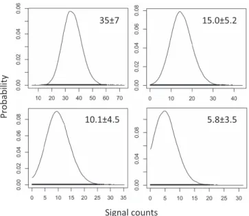
Suppose we perform a simple counting measurement. We have measured the total and the background counts, and we are interested in estimating the signal(i.e., total minus background) counts. When we set up a Bayesian model for this situation, it is appropriate to assume Poissonian likelihoods for both the total and the background counts. Figure 1 shows numerical results obtained usingJAGS. The panels display the posteriors for the signal counts. We assumed a uniform prior between 0 and 1000, i.e., the posterior will closely reflect the shape of the likelihood (see Equation (13)). The different panels are obtained for a total number of counts of 40, 20, 15, and 10, while the background counts are keptfixed at 5. The predicted mean and standard deviation of the signal are indicated in each panel. When the total number of counts is relatively large(e.g., 40; see first panel), the probability for predicting zero signal counts is negligible. In addition, the shape of the density function is well approximated by a lognormal distribution. On the other hand, when the total number of counts is similar to the background counts (e.g., 5; see last panel), the posterior predicts a large probability at zero signal counts and certainly does not resemble a lognormal distribution. The sequence of panels shows that the probability density can be approximated by a lognormal distribution as long as the ratio of mean value and standard deviation is3(see second panel). Similar results are obtained when different priors are used (e.g., gamma Figure 1. Posteriors of the signal (i.e., total minus background) counts, computed usingJAGS, for a hypothetical counting experiment. The panels are obtained for a total number of counts of 40(upper left), 20(upper right), 15 (lower left), and 10(lower right), while the background counts are keptfixed at 5. The predicted mean and standard deviation of the signal are indicated in each panel. A uniform distribution between 0 and 1000 is assumed for the prior.
functions, exponentials, or hyperpriors). Consequently, we will exclude from our analysis of experimental S-factors the few data points that do not satisfy this criterion.
3. BAYESIAN ASTROPHYSICALS-FACTORS
We will now apply the Bayesian method to the estimation of astrophysical S-factors10, S(E). This quantity is defined as (Iliadis2015)
s
º ph
S E( ) E ( )E e2 ( )4
wheres( )E is the nuclear reaction cross section at the center-of-mass energy, E. The quantity e2ph denotes the Gamow factor, given by
ph=
+ Z Z M M
M M E
2 0.98951013 0 1 0 1 1 5
0 1
( )
with Zi the charges of the projectile and target; in this expression, the relative atomic masses, Mi, and the energy,E, are in units of u and MeV, respectively.
The experimental S-factor can be extracted from data using fitting functions based either on a polynomial representation or on nuclear reaction models. The former provides a result that is independent of nuclear theory. Because this procedure has no theoretical justification beyond the known data points, it requires that theS-factor data cover the entire energy region of astrophysical interest. However, this is frequently not the case, especially at low bombarding energies, where the Coulomb barrier greatly inhibits direct measurements.
When data are missing in the region of interest, fitting functions motivated by nuclear theory (e.g., potential models, microscopic calculations, or R-matrix approaches)are usually preferred (Adelberger et al. 2011). With this method, it is assumed that the nuclear model reliably describes the energy
dependence of the S-factor, but that the absolute scale is
determined by a fit of the data using the nuclear model. The assumption of an additional normalization motivated by experimental data can be explained qualitatively. For example, many microscopic models compute the interior wavefunctions over truncated configuration spaces, with consequences for the normalization. Similarly, in ab initio models, small variations in the strength of the effective nucleon–nucleon interaction, which is adjusted to reproduce nucleon–nucleon scattering data, will result in changes of the S-factor normalization. Nevertheless, we emphasize that the need for an additional normalization has no rigorous theoretical justification. How-ever, since we cannot easily compute microscopic models and vary the model parameters, the assumption of a normalization factor determined by experiment represents the most straight-forward method. In any case, the extrapolation of theS-factor beyond the measured data will have some theoretical justification.
We will present in the following a Bayesian analysis for several light-particle nuclear reactions, assuming for the model
S-factor either a polynomial representation or the results of nuclear models. Each of these reactions has it own intricacies.
3.1. S-factor for d(p,g)3He
The reaction d(p,γ)3He represents the second step in the pp chains of stellar hydrogen burning. Since it occurs at a much faster than the first step, p(p,e+ν)d, uncertainties in the d(p,
γ)3He reaction are usually not important for stellar energy
generation. In special situations, however, this reaction does play a crucial role. For example, during the earliest stages of stellar evolution, when a cloud of interstellar gas collapses to form a protostar, the central temperature reaches a few million kelvin. At this temperature, primordial deuterium fuses with hydrogen (deuterium burning), thereby generating nuclear energy that slows the contraction and the central heating of the gas until the deuterium is consumed. The reaction d(p,γ)3He also plays a crucial role in Big Bang nucleosynthesis (Coc et al. 2015 and references therein), which begins when the temperature has declined to ≈0.9GK, corresponding to relevant kinetic energies of≈100 keV. The uncertainty in the d(p,γ)3He reaction rate impacts the primordial abundances of d,
3He, and7Li. For example, the reaction rate needs to be known
to better than ≈5% below an energy of 200 keV to compare predictions from Big Bang nucleosynthesis with the very precise value (uncertainty of 1.6%) of the deuterium-to-hydrogen(D/H)abundance ratio measured in very metal-poor, damped Lyα systems(Cooke et al.2014).
Most recently, S-factors and reaction rates for d(p,γ)3He have been presented by Coc et al.(2015). A reliable estimation ofS-factors requires simultaneous knowledge of statisticaland
systematic uncertainties, as discussed in Section 2.1. Among the many data sets published during 1962–2008, this informa-tion is available for only four studies(Ma et al.1997; Schmid et al.1997; Casella et al.2002; Bystritsky et al. 2008). These were the only data sets used by Coc et al. (2015) for their estimation of the S-factor, and we will apply the same data selection.11The data point at the lowest measured bombarding energy of Casella et al.(2002)has a ratio of the mean value to the standard deviation in excess of 3 and has been omitted in our analysis for the reasons given in Section 2.3. This data point was included in the analysis of Coc et al.(2015). The data adopted for the present analysis are displayed as black symbols in Figure 2, where the displayed error bars refer to (1s)
statisticaluncertainties only.
TheS-factorfit to the data was performed in previous work by using polynomials (e.g., Adelberger et al.2011)or results from nuclear theory (e.g., Descouvemont et al. 2004; Coc et al.2015). Similar to Coc et al.(2015), we will adopt in the present work the theoretical S-factors from Marcucci et al. (2005). They were obtained using variational wavefunctions for the p–d continuum and3He bound states, together with a Hamiltonian consisting of two-nucleon and three-nucleon potentials. We will assume that the theoretical model adequately describes the shape of theS-factor curve, but that the absolute scale of the modelS-factor is determined by thefit to the data.
TheJAGSmodel for each of the four data sets includes the effects of systematic uncertainties, robust regression, and lognormal likelihood functions, as discussed in Section 2. Our Bayesian model hasfive parameters. Four of these are the normalizations of the individual data sets. The highly
10
Analyzing S-factor data rather than cross section data has a number of advantages, among them a dramatic reduction in the energy dependence at the low bombarding energies considered here, and a straightforward comparison to literature results.
11
informative priors for these parameters are computed using systematic uncertainty factors of 1.09 (Ma et al. 1997), 1.09 (Schmid et al. 1997), 1.045 (Casella et al. 2002), and 1.08 (Bystritsky et al.2008), which are listed in Table I of Coc et al. (2015). The fifth parameter is the common scaling factor by which the results of the nuclear model have to be multiplied to fit the data. We assume a non-informative prior for this parameter, i.e., a normal probability density with a location of zero and a standard deviation of 100. The distribution was truncated at zero since the scaling factor must be a positive quantity. Other choices of priors (i.e., uniform and gamma functions) gave very similar results. The theoretical S-factor from Marcucci et al. (2005), available to us as a table of 100,000S-factor values between center-of-mass energies of 0.0 and 2.0 MeV, was directly implemented intoJAGS.
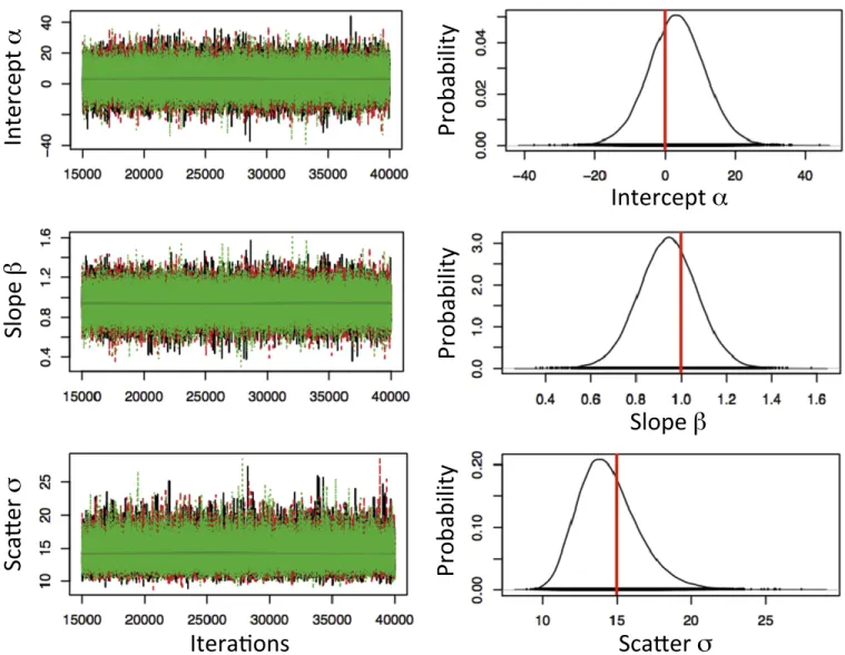
With our Bayesian model, we generated random samples using three independent Markov chains, each of length 75,000 (without burn-in). This ensures that the Monte Carlo fluctuations are negligible compared to the statistical and systematic uncertainties. A first impression can be obtained from Figure 2. The gray shaded region consists of lines that correspond to the credible S-factor curves, where each line corresponds to one sampled set of model parameters. The blue line represents the median(50th percentile), and the red lines the 16th and 84th percentiles of all credible S-factors. More information on the meaning of these lines can be found in AppendixA.
Details of our analysis are given in Table1and are compared to recently published results obtained using traditional statistics (c2 minimization). The top part of the table displays the normalization factors (“norm”) of each data set, taking into account the reported systematic uncertainties(see above). The present and previous values overlap within uncertainties. However, the magnitude of the uncertainties differs signifi -cantly. For example, for the data of Casella et al. (2002)our uncertainties are a factor of»4 larger than those of Coc et al.
Figure 2.AstrophysicalS-factor vs. center-of-mass energy for the d(p,γ)3He reaction. The symbols show the data of Ma et al.(1997, circles), Schmid et al.(1997, squares), Casella et al.(2002, triangles), and Bystritsky et al.(2008, diamonds). The error bars refer to(1s)statistical uncertainties only. The lines have the following meaning:(gray shaded area)credibleS-factors, obtained from the output of theJAGSmodel, where each line corresponds to one specific set of model parameters; (blue)median(50th percentile)of all credible lines;(red)16th and 84th percentiles of all credible lines. The credible lines are calculated from the theoreticalS-factor of Marcucci et al.(2005), multiplied by a scale factor that is a parameter of the Bayesian model. The data point at the lowest measured bombarding energy(not shown) of Casella et al.(2002), which has a ratio of the mean value to the standard deviation in excess of 3, has been omitted in our analysis(see text).
Table 1
Results for the Reaction d(p,γ)3He
Data Presenta Previousb
Ref.c nd Norme Outlierf Normg cn2h
Ma 97 4 0.895-+0.0480.058 24% 0.8469±0.0381 1.1052 Sch 97 7 0.981-+0.0410.041 72% 0.9657±0.0062 11.1799 Cas 02 51 1.025-+0.0370.038 1.3% 1.0243±0.0092 0.5792 Bys 08 3 1.023-+0.0680.072 12% 1.0365±0.1457 0.1360
Quantity Presenta Previousb
Scale factori: 1.000-+0.0360.038 0.9900±0.0368
S(0) (MeV b): (2.156-+0.0820.077)´10-7 (2.130.08)´10-7 ´
-+
-2.14 0.160.17 10 7
( ) j
´
-2.1 0.4 10 7
( ) k
Notes.
a
Uncertainties are derived from the 16th, 50th, and 84th percentiles of the probability density(posterior).
b
From Coc et al.(2015), unless mentioned otherwise. c
Reference labels: Ma 97(Ma et al.1997); Sch 97(Schmid et al.1997); Cas
02(Casella et al.2002); Bys 08(Bystritsky et al.2008).
d
Number of data points in a given set.
eNormalization of each data set, taking into account the reported systematic uncertainties(see text).
f
Probability that the data set is an outlier; computed from the average outlier probability of a given set.
g
Normalization of each data set, taking into account the reported systematic uncertainties(see text); the values represent1suncertainties.
h
Reducedc2. i
Best estimate for the scale factor of the theoreticalS-factor from Marcucci et al.(2005).
j
Zero-energyS-factor from Adelberger et al.(2011), which was obtained from ac2minimization of a quadraticS-factor parameterization.
k
Zero-energy S-factor from Xu et al.(2013), which was obtained using a potential model and ac2minimization.
(2015), while for the data of Bystritsky et al. (2008) our uncertainties are smaller by a factor of≈2. The fourth column summarizes the outlier probability of the different data sets. The values are computed from the average of the outlier probabilities of all data points in a given set, as predicted by
JAGS. The data of Schmid et al.(1997)have an average outlier probability of 72%, in agreement with the elevated reducedc2 found by Coc et al. (2015)for this set.
The same data sets were analyzed in both Coc et al.(2015) and the present work, and the same systematic uncertainties were adopted in both studies. Therefore, it is interesting to investigate the main reason for the significant differences, mentioned above, that are obtained in the analysis of the data of Casella et al.(2002)and Bystritsky et al.(2008). We performed a series of tests and found that neither inclusion or omission of the lowest-lying data point in Casella et al.(2002), nor the use of the correct or incorrect center-of-mass energies in Bystritsky et al. (2008) (see Footnote 10) had an effect on our derived normalization factors listed in the top part of Table 1. These changes in the data sets are too small to affect the analysis. We also performed a test by using Gaussian instead of lognormal likelihoods for the data points and obtained again results in agreement with those listed in Table 1. This is not surprising because, with few exceptions, the data points have relatively small error bars, implying that a Gaussian closely approximates the lognormal likelihood(Section 2.3). We thus conclude that the significant differences obtained currently and previously regarding the data sets of Casella et al. (2002)and Bystritsky et al.(2008)are caused by the adoption of a Bayesian model in our work as opposed to using a traditional method employed by Coc et al.(2015).
The lower part of Table1compares the present and previous values for the scale factor of the theoretical model results, and the astrophysicalS-factor at zero energy. Our Bayesian analysis verifies the results reported by Coc et al.(2015), for both the recommended values and the magnitude of the uncertainties. Our zero-energyS-factor also agrees with the value presented in Adelberger et al.(2011), although our uncertainty(3.7%)is smaller by a factor of 2. The analysis by Adelberger et al. (2011)was performed using ac2minimization and assuming a quadratic parameterization of theS-factor. The zero-energyS -factor presented in Xu et al. (2013) has a much larger uncertainty(19%)than all other recent values. It was obtained, using a potential model, from a standardc2 fit in conjunction with a“fit-by-eye”technique.
In summary, completely independent methods of analysis provide comparable results. But unlike the c2 minimization applied previously, the Bayesian technique provides consistent answers without the need to resort to Gaussian assumptions and other approximations. Thermonuclear reaction rates will be presented in Section 4.1.
3.2. 3He(3He,2p)4He
The reaction 3He(3He,2p)4He represents the third and final step of the pp1 chain. The competition of this process with the reaction 3He(α,γ)7Be determines the relative neutrino fluxes that originate from the pp and pep reactions (pp1 chain) compared to the7Be and8B decays(pp2 and pp3 chains). The
S-factor ratio for 3He(3He,2p)4He and 3He(α,γ)7Be enters directly in the calculation of the solar neutrino energy losses, and thus impacts the relationship between the photon
luminosity and the total energy production of the Sun (Adelberger et al.2011).
The astrophysicalS-factor of 3He(3He,2p)4He was recently evaluated by Adelberger et al.(2011). As discussed above and in that work, a reliable estimation of the astrophysicalS-factor requires separate knowledge of statistical and systematic uncertainties. This information is reported in four studies. The quoted systematic uncertainties are 4.5% (Krauss et al. 1987), 3.7% (Junker et al. 1998), 5.7% (Bonetti et al. 1999), and 3.8% (Kudomi et al. 2004). To these data we added one more study(Dwarakanath & Winkler1971)for which we could infer separate statistical (4%–7%) and systematic uncertainties (8.2%) based on the information provided. Our reasoning is discussed in more detail in Appendix C.2. The data adopted in the present work are displayed as black symbols in Figure3, where the displayed error bars refer to(1s)statisticaluncertainties only.
We disregarded the two data points from Bonetti et al. (1999)at center-of-mass energies of 16.50 and 17.46 keV, with reported S-factor values of 7.70±7.70 MeV b and 5.26±5.26 MeV b, respectively, for the reasons given in Section2.3. Only a single event was observed at each of these two energies, and the quoted errors refer to statistical uncertainties only(see their Table I). It would not be difficult to include such data in a Bayesian model if their probability
densities were known. Since this information is not provided by
Bonetti et al.(1999), we cannot include these two data points with very large errors. They should also not be included in a traditional(c2minimization)analysis. Bonetti et al.(1999)and Adelberger et al.(2011)do not mention whether they included these two data points or not.
TheS-factorfit to the data was performed in previous work (Bonetti et al. 1999; Adelberger et al. 2011) by using the expressions
= ph
S E Sbare E e 6
Ue E
( )
( ) ( ) ( )
= + ¢ +
S E S 0 S 0 E 1S E
2 0 7
bare( ) ( ) ( ) ( ) 2 ( )
whereSbareis the bare-nucleusS-factor that is not influenced by
electron screening,S(0) is theS-factor at zero center-of-mass energy, S¢( )0 and S( )0 are the first and second energy derivatives of the S-factor at zero energy, and Ue is the electron-screening potential energy. This expression adequately describes the total measured S-factor, S(E), at energies below 1.1 MeV.
Our Bayesian model has nine parameters. Five of these are the normalizations of the individual data sets. The highly informative priors for these parameters are computed using the systematic uncertainty factors quoted above. The other parameters are S(0), S¢( )0, S( )0 , and Ue. We assume non-informative priors for these parameters, i.e., normal probability densities located at zero with large values for the standard deviations. The distributions forS(0)andUewere truncated at zero energy since both theS-factor and the electron-screening potential energy are positive quantities. Other choices of priors gave consistent results.
gray lines)electron-screening corrections. All other lines have the same meaning as in Figure2.
Our results are listed in Table 2 and they are compared to recently published values obtained using traditional statistics (c2 minimization). The top part of the table displays the normalization factors (“norm”) of each data set, taking into account the reported systematic uncertainties(see above). The fourth column summarizes the outlier probability of the different data sets, which is computed from the average of the outlier probabilities of all data points in a given set, as predicted byJAGS. Wefind the largest outlier probabilities for the data of Krauss et al. (1987) (67%) and Bonetti et al. (1999) (58%).
The lower part of Table2compares the present and previous values for the S-factor expansion coefficients, S(0), S¢( )0,
S ( )0, and the electron-screening potential,Ue. Notice that each of the listed present values is marginalized over all other parameters(see AppendixB). Our results agree with those of Bonetti et al.(1999)within uncertainties. However, our values forS¢( )0 andS( )0 disagree with those reported by Adelberger et al.(2011). Since their value ofS(0)agrees with our result, we conclude that the disagreement for the other parameters is caused by the significantly smaller range of bombarding energy analyzed by Adelberger et al. (2011), i.e., 0–350 keV, compared to 0–1.1 MeV in the present work. Our uncertainty of 2.6% for the zero-energyS-factor is much smaller than the value of 9.4% reported by Xu et al.(2013), who obtained theS -factor using a phenomenological nuclear reaction model and a c2 minimization.
Furthermore, Adelberger et al. (2011)report anS-factor of
=
SAdelberger(E0) 5.11 0.22MeV b at the Gamow peak
(E0=21.94 keV) for the Sun’s central temperature
(T=15.5 MK), corresponding to an uncertainty of 4.3%. Our result isSpresent(E0)=5.08-+0.130.14MeV b, corresponding to a
significantly smaller uncertainty of 2.7%. Thermonuclear reaction rates will be presented in Section4.2.
3.3.3He(α,g)7Be
The detection of solar neutrinos has entered a precision era, enabling the measurement of neutrino fluxes with a total uncertainty of about 3%–5% by various neutrino detectors (Aharmin et al. 2013; Smy 2013; Bellini et al. 2014). The measured neutrinofluxes can be used to probe the solar core and test solar models, provided that the relevant thermonuclear reaction rates are accurately known. Since the reaction3He(α,
γ)7Be competes with 3He(3He,2p)4He, it determines the
number of 7Be and 8B neutrinos originating from the pp2 and pp3 chains. The reaction 3He(α,γ)7Be also plays a prominent role in Big Bang nucleosynthesis. While the primordial abundances of d, 3He, and 4He predicted by standard Big Bang models are in reasonable agreement with those from observation, the models overproduce the primordial abundance of 7Li by a factor of ≈3. This “7Li problem” is among the unsolved mysteries in astrophysics (Iocco et al.2009). Most of the 7Li in the early universe is produced as7Be, by the reaction3He(α,γ)7Be, and decays subsequently via electron capture to7Li. Although a new determination of the rate of 3He(α,γ)7Be does not appear to solve the 7Li problem, it is nevertheless desirable to determine a reliable rate for this reaction.
Many groups have measured the reaction3He(α,γ)7Be using various experimental strategies. For summary discussions, see Adelberger et al.(2011), Bordeanu et al.(2013), and deBoer et al. (2014). Similar to the procedure in Adelberger et al. (2011), we adopt a subset of all published measurements for the present analysis. First, we consider only those studies that provide separate statistical and systematic uncertainties. This excludes all measurements performed before the year 2000. Figure 3.AstrophysicalS-factor vs. center-of-mass energy for the3He(3He,2p)4He reaction. The symbols show the data of Dwarakanath & Winkler(1971, circles), Krauss et al.(1987, diamonds), Junker et al.(1998, squares), Bonetti et al.(1999, inverted triangles), and Kudomi et al.(2004, triangles). The error bars refer to(1s)
statistical uncertainties only. The lines have the following meaning:(gray shaded area)credibleS-factors, obtained from the output of theJAGSmodel, where each line corresponds to one specific set of model parameters;(blue)median(50th percentile)of all credible lines;(red)16th and 84th percentiles of all credible lines. The upper gray lines are calculated using a quadratic expansion of the bare-nucleusS-factor, multiplied by an exponential factor that takes into account laboratory electron screening(see text). The lower gray lines represent the bare-nucleusS-factor(i.e., without electron-screening corrections). Two data points(not shown)at the lowest measured bombarding energies of Bonetti et al.(1999), which have ratios of the mean value to the standard deviation in excess of 3, have been omitted from our analysis(see text).
Second, we focus on the center-of-mass energy region below 1.6 MeV. Third, we consider only those experiments that directly measure the total cross section, i.e., via activation or recoil detection. We exclude prompt γ-ray data, since these studies rely so far on computed rather than measured corrections for γ-ray angular correlation effects. Based on these selection criteria, four data sets remain: Brown et al. (2007), Nara Singh et al. (2004), Di Leva et al. (2009), and Costantini et al. (2008), which were labeled “Seattle,” “Weizmann,” “ERNA,”and “LUNA,” respectively, in Adel-berger et al. (2011). For systematic uncertainties, we adopt 3.0%(Brown et al.2007), 5.1%(Nara Singh et al.2004), 5.0% (Di Leva et al.2009), and 3.1%(Costantini et al.2008). Notice that Adelberger et al.(2011)adopt a systematic uncertainty of only 2.2% for the data of Nara Singh et al.(2004). However, this value applies to their highest-energy data point only, while the other three data points have considerably higher systematic uncertainties (4.1%–7.1%). We adopt here the average value. The data adopted in the present work are displayed as black symbols in Figure 4, where the displayed error bars refer to (1s)statistical uncertainties only.
Several different strategies have been employed in the past to fit the experimental S-factor data for the reaction 3He(α,
γ)7Be, including potential models(Tombrello & Parker1963),
parameterized analytical functions (Cyburt & Davids 2008), resonating-group methods (Kajino 1986), and R-matrix approaches(deBoer et al.2014). In this work, we will focus on three microscopic models. Thefirst is the resonating-group study of Kajino (1986), which has been used in several previous investigations. In this model, the nuclear system is characterized by antisymmetrized wavefunctions describing the relative motion of two clusters. The required phenomen-ological nucleon–nucleon interactions were tuned to repro-duce the properties of bound and scattering states within the restricted cluster model space. The second is the calculation of Nollett (2001), which employed accurate nucleon–nucleon potentials. The bound states were computed using the variational Monte Carlo method, while the relative motion of the nuclei in the initial state was described by one-body wavefunctions generated from the intercluster potential A of Kim et al. (1981). The third is the ab initio model of Neff (2011), which employed realistic interactions to solve the many-body problem using a large model space. The latter work found that the assumption of a predominant external capture, which was commonly adopted in most previous studies, is not that well satisfied. Similar to the discussion in Section3.1, we assume that these models adequately describe the shape of the S-factor, but that the absolute scale of each model S-factor is determined by a fit to the data. In the following, we first discuss and quote results obtained using the model of Neff(2011). Subsequently, we use the models of Kajino (1986) and Nollett (2001) to estimate the model uncertainty for the extrapolation of the S-factor to low energies, where no data exist. We obtained the theoreticalS -factors for all three models from the original authors as numerical tables, which were directly implemented into
JAGS. Tests showed that this procedure caused negligible errors in the linear interpolation between grid points.
Our Bayesian model hasfive parameters. Four of these are the normalizations of the individual data sets. The highly informative priors for these parameters are computed using the systematic uncertainty factors quoted above. The fifth para-meter is the common scaling factor by which the nuclear model results have to be multiplied tofit the data. We assume a non-informative prior for the latter parameter, i.e., a normal probability density with a location of zero and a standard deviation of 100. The distribution was truncated at zero since the scaling factor must be a positive quantity. Other choices of priors gave very similar results. We generated random samples using three independent Markov chains, each of length 75,000 (without burn-in). Results are shown in Figure 4, where the lines have the same meaning as in Figure2.
Our numerical results are listed in Table3and are compared to recently published values obtained using different methods. The top part of the table displays the normalization factors (“norm”) of each data set, taking into account the reported systematic uncertainties (see above). The fourth column summarizes the outlier probability of the different data sets, which is computed from the average of the outlier probabilities of all data points in a given set, as predicted by JAGS. We obtain the largest average outlier probability for the data of Brown et al.(2007) (81%).
The lower part of Table3compares the present and previous values for theS-factor at zero energy,S(0). Fromfitting the data using the model of Neff (2011), we find S( )0present= Table 2
Results for the Reaction3He(3He,2p)4He
Data Presenta Ref.b nc Normd Outliere
Dwa 71 17 1.000-+0.0310.032 18% Kra 87 47 0.977-+0.0210.022 67% Jun 98 25 1.040-+0.0220.023 14% Bon 99 8 0.955-+0.0400.044 58% Kud 04 8 0.991-+0.0220.023 31%
Quantity Presenta,f Previousg Previoush
S(0) (MeV b): 5.14-+0.140.13 5.32±0.08 5.32±0.23 ¢
S( )0 (b): -2.69-+0.540.54 −3.7±0.6 −6.44±1.29
S ( )0 (b/MeV): 2.14-+0.910.89 3.9±1.0 30.7±12.2
Ue(eV): 325-+4748 294±47 280±70
S E( 0=21.94 keV)(MeV b)i:
-+
5.08 0.130.14 5.11±0.22
Notes.
a
Uncertainties are derived from the 16th, 50th, and 84th percentiles of the probability density(posterior).
b
Reference labels: Dwa 71(Dwarakanath & Winkler1971); Kra 87(Krauss et al.1987); Jun 98(Junker et al.1998); Bon 99(Bonetti et al.1999); Kud 04 (Kudomi et al.2004).
c
Number of data points in a given set. d
Normalization of each data set, taking into account the reported systematic uncertainties (see text); the values correspond to 16th, 50th, and 84th percentiles of the probability density(posterior).
e
Probability that the data set is an outlier; computed from the average outlier probability of a given set.
f
Fit is valid for center-of-mass energies of1.1 MeV;each quoted value is marginalized over all other parameters(see text).
g
Fromc2minimization of Bonetti et al.(1999, see their Table II). h
Fromc2 minimization of Adelberger et al. (2011), using their quadratic representation of the bare-nucleusS-factor(see their Table II).
i
(5.72±0.12)×10−4 MeV b, representing an uncertainty of 2.1%. Our result agrees within the quoted uncertainties with those of Adelberger et al.(2011), who used the same data sets in their analysis as we did. Notice, however, that Adelberger et al.(2011) employed an analytic function that approximated theS-factor of Nollett(2001)“to better than 0.3%, on average.”In contrast, we directly used the original numerical tables of Neff (2011) and there was no need for an approximation. Compared to Adelberger et al. (2011), our uncertainty in S(0) from fitting the data is smaller by a factor of≈2. It is also interesting that our value forS
(0) disagrees with the R-matrix result of deBoer et al. (2014),
S( )0 deBoer=(5.42± 0.11)×10−4MeV b, where their quoted error is based on the datafit only. Their quoted mean value ofS
(0)is lower by 5.5% than our result.
For low energies, especially those pertaining to the solar Gamow peak, data do not exist and the S-factor must be extrapolated to compute the reaction rates. Therefore, past work has included a“theory error”that is based on the spread inS(0) values obtained when different theoretical models are used tofit the data. In our case, we repeated our analysis using the theoretical model S-factors of Kajino (1986) and Nollett (2001). With the theoretical model of Nollett (2001), we find almost identicalS -factors (mean value and uncertainties) to the model of Neff (2011). The model of Kajino (1986) resulted in a similar uncertainty, but a mean value smaller by a factor of 2.2%. Using the full spread of 2.2% as an estimate for the“theory error,”our result is S( )0 present=(5.72±0.12(exp)±0.13(theo))×10−4 MeV b. This can be compared to S( )0Adelberger=(5.6±0.2 (exp)±0.2(theo))×10−4MeV b andS( )0 deBoer=(5.42±0.11 (MCfit)±0.06(model) +-0.110.19(phase shifts))×10−4 MeV b.
Concerning the result of deBoer et al.(2014), thefirst uncertainty was obtained from the data fit, the second from varying the background pole energies and the R-matrix channel radius, and the third from using different scattering data sets to define the phase shifts. Thermonuclear reaction rates will be presented in Section4.2.
Figure 4.AstrophysicalS-factor vs. center-of-mass energy for thereaction3He(α,γ)7Be. The symbols show the data of Costantini et al.(2008, circles), Brown et al.
(2007, diamonds), Nara Singh et al.(2004, squares), and Di Leva et al.(2009, inverted triangles). The error bars refer to(1s)statistical uncertainties only. The lines have the following meaning:(gray shaded area)credibleS-factors, obtained from the output of theJAGSmodel, where each line corresponds to one specific set of model parameters;(blue)median(50th percentile)of all credible lines;(red)16th and 84th percentiles of all credible lines. The credible lines are calculated from the theoreticalS-factor of Neff(2011), multiplied by a scale factor that is a parameter in the Bayesian model. Notice the linear scale, unlike the previousfigures, for better comparison with other plots of3He(α,γ)7BeS-factor published recently.
Table 3
Results for the3He(α,γ)7Be Reaction
Data Presenta Ref.b nc Normd Outliere
Nar 04 4 0.966-+0.0250.026 36% Bro 07 8 1.031-+0.0230.024 81% Cos 08 6 0.977-+0.0210.022 28% DiL 09 15 1.003-+0.0210.022 9.0%
Quantity Presenta Previous
Scale factorf: 0.964-+0.0200.021
S(0) (MeV b): (5.720.12)´10-4g (5.60.2)´10-4h
(5.42±0.11)×10−4i
Notes.
a
Uncertainties are derived from the 16th, 50th, and 84th percentiles of the probability density(posterior).
b
Reference labels: Nar 04 (Nara Singh et al. 2004); Bro 07 (Brown
et al.2007); Cos 08(Costantini et al.2008); DiL 09(Di Leva et al.2009).
cNumber of data points in a given set. d
Normalization of each data set, taking into account the reported systematic uncertainties(see text).
e
Probability that the data set is an outlier; computed from the average of the outlier probabilities of all data points in a given set.
f
Best estimate for the scale factor of the theoreticalS-factor from Neff(2011). g
Uncertainty from datafit using the theoreticalS-factor from Neff(2011)only; an additional“theory uncertainty” of0.12´10-4 MeV b is found when different theoretical models are used(see text).
h
From Adelberger et al.(2011); the originalS-factor quoted in that work isS
(0)=0.56±0.02(exp)±0.02(theo)keV b, where the latter uncertainty contribution was obtained for a range of theoretical models.
i
From deBoer et al.(2014); the originalS-factor quoted in that work is S
(0)=0.542±0.011(MCfit)±0.006(model)-+0.0110.019(phase shifts)keV b; the
first uncertainty was obtained from the datafit, the second from varying the background pole energies and the R-matrix channel radius, and the third from using different scattering data sets to define the phase shifts.
4. BAYESIAN REACTION RATES
The thermonuclear reaction rate per particle pair, NAá ñsv,
can be written as(Iliadis2015)
⎛ ⎝
⎜ ⎞⎠⎟
ò
s p
á ñ =
ph
¥
-
-N v
m
N kT
e S E e dE 8
8 A
A
E kT
01 1 2
3 2
0 2
( )
( ) ( )
wherem01is the reduced mass of projectile and target, andNA is Avogadro’s constant; the product of Boltzmann constant, k, and plasma temperature, T, is numerically given by
=
kT 0.086173324T9(MeV) ( )9
with the temperature, T9, given in units of GK.
For each set of parameters sampled by the MCMC algorithm, we calculate the reaction rates by numerical integration of Equation (8) on a grid of 60 temperatures between 1MK and 10GK. The resulting set of values of the reaction rate constitute the probability density at a given temperature. Using this probability density, we follow the procedure recommended in Longland et al.(2010)to compute a recommended rate (50th percentile), a high rate and low rate (16th and 84th percentiles, respectively), and the lognormal parameters, μ and σ, of the lognormal approximation of the total reaction rate. The rate factor uncertainty, f u. ., corresp-onding to a coverage probability of 68%, is obtained from
f u. .=es (see Equation (1)). Notice that we directly compute the lognormal parameters from the expectation value and variance of all rate samples, ln(NAá ñsvi), at a given
temper-ature. This ensures that the results can be directly incorporated into the STARLIB library(Sallaska et al.2013).
4.1. Reaction Rates for d(p,g)3He
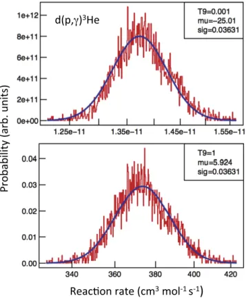
The present rates for the reaction d(p,γ)3He, together with the corresponding factor uncertainties, are listed in columns 2 and 3 of Table4. The rate factor uncertainty is constant, f u. .=3.7% (except at the highest temperatures; see below), since it is determined by a single parameter (i.e., the common scaling factor; Section3.1). Probability densities of the reaction rate are shown in Figure 5 for two selected temperatures, T=1MK (top), near the range important for deuterium burning, and
T=1GK(bottom), relevant for Big Bang nucleosynthesis. The reaction rate samples(red histograms)are computed using theS -factor samples obtained from the Bayesian model(Section3.1). The sampled rates are well represented by lognormal probability densities, shown as blue curves.
For temperatures of T 8MK, our rates agree with the recently evaluated results of Coc et al. (2015) within 1%. However, at lower temperatures, important for deuterium burning, our rates deviate strongly from the previous results. For example, at the lowest temperature, T=1MK, our rates are larger by a factor of≈300 than those of Coc et al.(2015).12 The disagreement is explained by an erroneously assumed lower integration limit of 2 keV in the previous work, which is too high for computing the reaction rates at the lowest temperatures. Our estimated reaction rate factor uncertainties are close to the values given previously at all temperatures. We integrate the reaction rates numerically only up to 2 MeV, i.e.,
the highest center-of-mass energy for which we have theor-eticalS-factors from Marcucci et al.(2005). Since we may miss rate contributions at the highest temperatures,T 5GK, we adopt in this region the values from Coc et al.(2015), which are shown in italics in Table4.
It is straightforward to calculate the effect of the new reaction rate on the predicted primordial D/H ratio. Our mean value for the scale factor (Table 1) represents a 1% increase compared to Coc et al.(2015). This difference translates into a decrease of the central D/H value by only 0.32% (Iocco et al. 2009), while the total uncertainty remains unchanged at 2%.
4.2. Reaction Rates for3He(3He,2p)4He
The present rates for thereaction 3He(3He,2p)4He, together with the corresponding factor uncertainties, are listed in columns 4 and 5 of Table 4. The rate factor uncertainties amount to 2.2%–2.7% for temperatures of T1.25GK. The reaction rate is shown in Figure6(top)for the temperature at the Sun’s center (15.5 MK). The reaction rate samples (red histograms)are computed using theS-factor samples obtained from the Bayesian model(Section 3.2). The sampled rates are well represented by a lognormal probability density, shown as blue curve.
Although for temperatures of T1.25GK our rates agree with those of Angulo et al.(1999), our estimated reaction rate factor uncertainties are significantly smaller, by a factor of
»2.7 (i.e., »2.4% versus »6.5%). Since we numerically integrate the reaction rates only up to 1.1 MeV, we may miss rate contributions at the highest temperatures, T >1.25GK. Therefore, we adopt in this region the values from Angulo et al. (1999), which are shown in italics in Table 4.
At temperatures relevant for the center of the Sun (T ≈
15.5 MK), the7Be and8B solar neutrinofluxes approximately scale with the S(0) value according to the relations fn7Be ∼
-S( )0 0.43 and f
nB 8
∼ S( )0-0.40 (Table XV in Bahcall & Ulrich 1988). Therefore, compared to the rate of Adelberger et al.(2011), our results translate into increases in the7Be and
8B solar neutrino fluxes by 1.5% and 1.4%, respectively. A
more detailed analysis, incorporating our much reduced uncertainty in S(0) (by factor of 2), is beyond the scope of the present work.
4.3. Reaction Rates for3He(α,g)7Be
The present rates for the reaction3He(α,γ)7Be, together with the corresponding factor uncertainties, are listed in columns 6 and 7 of Table4. The rate factor uncertainty amounts to 2.4% for temperatures ofT2.0GK. The probability density of the reaction rate is shown in Figure6(bottom)for the temperature at the Sun’s center (15.5 MK). The reaction rate samples (red histograms)are computed using theS-factor samples obtained from the Bayesian model(Section 3.3). The sampled rates are well represented by a lognormal probability density, shown as the blue curve.
For the Sun’s central temperature, the present reaction rates barely agree with the R-matrix results of deBoer et al.(2014) within the quoted uncertainties (corresponding to 68% probability density intervals). However, our recommended rate is larger by 6.0%. At Big Bang temperatures (≈1 GK), our result is in good agreement with the rate of deBoer et al. (2014). As already mentioned, wefit theS-factor data up to an
Table 4
Present Recommended Reaction Ratesa
d(p,γ)3He 3He(3He,2p)4He 3He(α,γ)7Be
T(GK) Rateb f u. .b Ratec f u. .c Rated f u. .d
0.001 1.379E–11 1.037 2.700E–41 1.025 1.178E–47 1.024
0.002 1.906E–08 1.037 1.694E–30 1.025 2.300E–36 1.024
0.003 6.175E–07 1.037 2.890E–25 1.025 6.811E–31 1.024
0.004 5.464E–06 1.037 5.721E–22 1.025 1.911E–27 1.024
0.005 2.557E–05 1.037 1.259E–19 1.025 5.391E–25 1.024
0.006 8.262E–05 1.037 7.683E–18 1.025 3.975E–23 1.024
0.007 2.101E–04 1.037 2.043E–16 1.025 1.230E–21 1.024
0.008 4.529E–04 1.037 3.052E–15 1.025 2.083E–20 1.024
0.009 8.655E–04 1.037 2.997E–14 1.025 2.273E–19 1.024
0.010 1.510E–03 1.037 2.140E–13 1.025 1.778E–18 1.024
0.011 2.456E–03 1.037 1.193E–12 1.025 1.073E–17 1.024
0.012 3.773E–03 1.037 5.451E–12 1.025 5.266E–17 1.024
0.013 5.538E–03 1.037 2.120E–11 1.025 2.182E–16 1.024
0.014 7.825E–03 1.037 7.209E–11 1.025 7.859E–16 1.024
0.015 1.071E–02 1.037 2.191E–10 1.025 2.517E–15 1.024
0.016 1.427E–02 1.037 6.051E–10 1.025 7.291E–15 1.024
0.018 2.368E–02 1.037 3.647E–09 1.025 4.782E–14 1.024
0.020 3.662E–02 1.037 1.711E–08 1.025 2.413E–13 1.024
0.025 8.760E–02 1.037 3.765E–07 1.024 6.141E–12 1.024
0.030 1.702E–01 1.037 3.957E–06 1.024 7.209E–11 1.024
0.040 4.480E–01 1.037 1.207E–04 1.024 2.582E–09 1.024
0.050 8.922E–01 1.037 1.359E–03 1.024 3.258E–08 1.024
0.060 1.511E+00 1.037 8.560E–03 1.024 2.238E–07 1.024
0.070 2.304E+00 1.037 3.705E–02 1.023 1.038E–06 1.024
0.080 3.267E+00 1.037 1.236E–01 1.023 3.666E–06 1.024
0.090 4.395E+00 1.037 3.414E–01 1.023 1.062E–05 1.024
0.100 5.680E+00 1.037 8.172E–01 1.023 2.648E–05 1.024
0.110 7.115E+00 1.037 1.749E+00 1.023 5.876E–05 1.024
0.120 8.693E+00 1.037 3.426E+00 1.023 1.187E–04 1.024
0.130 1.041E+01 1.037 6.240E+00 1.023 2.224E–04 1.024
0.140 1.225E+01 1.037 1.070E+01 1.023 3.913E–04 1.024
0.150 1.421E+01 1.037 1.746E+01 1.022 6.530E–04 1.024
0.160 1.629E+01 1.037 2.729E+01 1.022 1.042E–03 1.024
0.180 2.078E+01 1.037 6.000E+01 1.022 2.376E–03 1.024
0.200 2.567E+01 1.037 1.180E+02 1.022 4.818E–03 1.024
0.250 3.945E+01 1.037 4.534E+02 1.022 1.968E–02 1.024
0.300 5.510E+01 1.037 1.255E+03 1.022 5.698E–02 1.024
0.350 7.231E+01 1.037 2.813E+03 1.022 1.322E–01 1.024
0.400 9.084E+01 1.037 5.448E+03 1.022 2.631E–01 1.024
0.450 1.105E+02 1.037 9.492E+03 1.023 4.687E–01 1.024
0.500 1.311E+02 1.037 1.526E+04 1.023 7.677E–01 1.024
0.600 1.749E+02 1.037 3.316E+04 1.024 1.717E+00 1.024
0.700 2.215E+02 1.037 6.120E+04 1.024 3.239E+00 1.024
0.800 2.703E+02 1.037 1.009E+05 1.025 5.435E+00 1.024
0.900 3.211E+02 1.037 1.534E+05 1.025 8.380E+00 1.024
1.000 3.734E+02 1.037 2.193E+05 1.026 1.213E+01 1.024
1.250 5.101E+02 1.037 4.430E+05 1.027 2.519E+01 1.024
1.500 6.534E+02 1.037 7.96E+05 1.076 4.360E+01 1.024
1.750 8.017E+02 1.037 1.21E+06 1.077 6.717E+01 1.024
2.000 9.540E+02 1.037 1.70E+06 1.079 9.539E+01 1.024
2.500 1.268E+03 1.037 2.90E+06 1.081 1.705E+02 1.035
3.000 1.590E+03 1.037 4.32E+06 1.082 2.585E+02 1.035
3.500 1.916E+03 1.037 5.95E+06 1.081 3.602E+02 1.035
4.000 2.241E+03 1.037 7.75E+06 1.081 4.742E+02 1.035
5.000 2.905E+03 1.040 1.18E+07 1.079 7.351E+02 1.035
6.000 3.557E+03 1.042 1.63E+07 1.077 1.035E+03 1.035
7.000 4.194E+03 1.044 2.12E+07 1.073 1.370E+03 1.035
8.000 4.812E+03 1.046 2.63E+07 1.069 1.738E+03 1.035
9.000 5.410E+03 1.047 3.15E+07 1.067 2.135E+03 1.035
10.000 5.988E+03 1.049 3.68E+07 1.063 2.558E+03 1.035
Notes.
aIn units of cm3mol−1s−1. The values correspond to themedianrate, i.e., the 50th percentile of the probability density of the reaction rate. The rate factor uncertainty,f u. ., corresponding to
a coverage probability of 68%, is calculated fromf u. .=es, whereσdenotes the spread parameter of the lognormal approximation to the probability density of the reaction rate(see Equation(1)).
b
Values forT5GK, shown in italics, are adopted from Coc et al.(2015) (see text).
c
Values forT1.5GK, shown in italics, are adopted from Angulo et al.(1999) (see text).
d
Values forT2.5GK, shown in italics, are adopted from Kontos et al.(2013) (see text).
energy of 1.6 MeV. Therefore, we can only compute the reaction rates up to a temperature of 2.0GK. For higher temperatures, we adopt the values from Kontos et al. (2013), which are shown in italics in Table4.
At temperatures relevant for the center of the Sun (T ≈
15.5 MK), the7Be and8B solar neutrinofluxes approximately scale with the S(0) value according to the relations fn7Be ∼
S( )00.86andf
nB 8
∼S( )0 0.81(Bahcall & Ulrich1988). Therefore, compared to the rate of deBoer et al. (2014), our results translate into increases in the 7Be and8B solar neutrinofluxes by 4.7% and 4.5%, respectively.
The rate for3He(α,γ)7Be is the major nuclear physics source of uncertainty for the prediction of the primordial 7Li abundance. The 7Li/H ratio varies almost linearly with the reaction rate (Iocco et al. 2009). The study of primordial nucleosynthesis by Coc et al.(2015)adopted the rate of deBoer et al. (2014), which agrees with our result at Big Bang temperatures within a few per cent. Therefore, we expect only minor modifications to the predicted primordial 7Li/H ratio. Such small variations are negligible compared to the factor of 3 discrepancy between predicted and observed primordial7Li/H ratios, and thus are not relevant for the7Li problem.
5. SUMMARY
We discussed astrophysical S-factors and reaction rates based on Bayesian statistics, and developed a framework that incorporates robust parameter estimation, systematic effects,
and non-Gaussian uncertainties. Unlike the c2 minimization applied previously, the Bayesian technique provides consistent answers without the need to resort to Gaussian assumptions and other frequently applied approximations. The method is used to estimate the S-factors and reaction rates of d(p,γ)3He, 3He (3
He,2p)4He, and 3He(α,γ)7Be, important for deuterium burning, solar neutrinos, and Big Bang nucleosynthesis.
For the reaction d(p, γ)3He, our analysis verifies the results reported by Coc et al.(2015), for both the recommended values and the magnitude of the uncertainties. Our zero-energy S -factor also agrees with the value presented in Adelberger et al. (2011), although our uncertainty is smaller by a factor of ≈2. The zero-energy S-factor presented in Xu et al. (2013) has a much larger uncertainty(19%)than all other recently published values. Our reaction rate factor uncertainty is 3.7% for all temperatures below 5GK. Compared to Coc et al.(2015), our reaction rate at Big Bang temperatures is larger by about 1%. This translates into a decrease in the primordial D/H value by only 0.32%, while the total uncertainty remains unchanged at 2%.
For the reaction3He(3He,2p)4He, our results agree with those of Bonetti et al. (1999) within uncertainties. However, our parameter values forS¢( )0 andS( )0 disagree with those reported by Adelberger et al.(2011). Our uncertainty of 2.6% for the zero-energyS-factor is much smaller than the value of 9.4% reported by Xu et al.(2013). Furthermore, Adelberger et al.(2011)report anS-factor ofSAdelberger(E0)=5.11±0.22 MeV b at the Gamow peak (E0=21.94 keV) for the Sun’s central temperature
(T=15.5 MK), corresponding to an uncertainty of 4.3%. Our Figure 5.Probability densities of the reaction rate for the reaction d(p,γ)3He for
two temperatures (“T9”is in units of GK):(top)T=1MK, near the range important for deuterium burning;(bottom)T=1GK, relevant for Big Bang nucleosynthesis. Rate samples(red histograms)are computed using theS-factor samples obtained from the Bayesian model. Blue curves represent lognormal approximations, where the lognormal parametersμ(“mu”)andσ(“sig”)are directly calculated from the expectation value and variance of all rate samples,
s á ñ N v
ln( A i), at a given temperature.
Figure 6.Probability density of the reaction rate of(top)3He(3He,2p)4He and (bottom)3He(α,γ)7Be, for the temperature at the Sun’s center(15.5 MK). The rate samples(red histograms)are computed using theS-factor samples obtained from the Bayesian model. The blue curve represents a lognormal approx-imation, where the lognormal parametersμ(“mu”)andσ(“sig”)are directly calculated from the expectation value and variance of all rate samples,
s á ñ N v