rsos.royalsocietypublishing.org
Research
Cite this article:Leitão JC, Miotto JM, Gerlach M, Altmann EG. 2016 Is this scaling nonlinear?R. Soc. open sci.3: 150649. http://dx.doi.org/10.1098/rsos.150649
Received: 30 November 2015 Accepted: 15 June 2016
Subject Category:
Mathematics
Subject Areas:
statistics/fractals
Keywords:
scaling laws, statistical inference, allometry
Author for correspondence:
E. G. Altmann
e-mail:[email protected]
One contribution to a special feature ‘City
analytics: mathematical modelling and
computational analytics for urban behaviour’.
Is this scaling nonlinear?
J. C. Leitão, J. M. Miotto, M. Gerlach and E. G. Altmann
Max Planck Institute for the Physics of Complex Systems, Dresden, Germany
JCL, 0000-0003-1503-9242; JMM, 0000-0002-5850-3394; MG, 0000-0002-0879-7865; EGA, 0000-0002-1932-3710
One of the most celebrated findings in complex systems in the last decade is that different indexesy (e.g. patents) scale nonlinearly with the populationxof the cities in which they appear, i.e.y∼xβ,β=1. More recently, the generality of this finding has been questioned in studies that used new databases and different definitions of city boundaries. In this paper, we investigate the existence of nonlinear scaling, using a probabilistic framework in which fluctuations are accounted for explicitly. In particular, we show that this allows not only to (i) estimateβand confidence intervals, but also to (ii) quantify the evidence in favour ofβ=1 and (iii) test the hypothesis that the observations are compatible with the nonlinear scaling. We employ this framework to compare five different models to 15 different datasets and we find that the answers to points (i)–(iii) crucially depend on the fluctuations contained in the data, on how they are modelled, and on the fact that the city sizes are heavy-tailed distributed.
1. Introduction
The study of statistical and dynamical properties of cities from a complex-systems perspective is increasingly popular [1]. A celebrated result is the scaling between a city-specific observationy(e.g. the number of patents filed in the city) and the populationxof the city as [2]
y=αxβ, (1.1)
with a non-trivial (β=1) exponent. Super-linear scaling (β >1) was observed whenyquantifies creative or economic outputs and indicates that the concentration of people in large cities leads to an increase in theper capita(y/x) production. Sublinear scaling (β <1) was observed whenyquantifies resource use and suggests that large cities are more efficient in theper capita(y/x) consumption. Since its proposal, nonlinear scaling has been reported in an impressive variety of different aspects of cities [3–9]. It has also inspired the proposal of different generative processes to explain its ubiquitous occurrence [10–14]. Scalings similar to the one in equation (1.1) appear in physical (e.g. phase transitions) and biological (e.g. allometric scaling) systems suggesting that cities share similarities with these and other complex systems (e.g. fractals).
More recent results cast doubts on the significance of the β=1 observations [15–17]. Reference [15] agrees that economic
2
rsos
.ro
yalsociet
ypublishing
.or
g
R.
Soc
.open
sc
i.
3
:1
50649
...
1 10 102 103 104
103
104
105
106 107 108
103
102
104
105
106 107
108
USA Brazil Europe UK
105 106 107
y = x
population
rank
y
=
cinema usage
x= population
OECD
European cities
(b) (a)
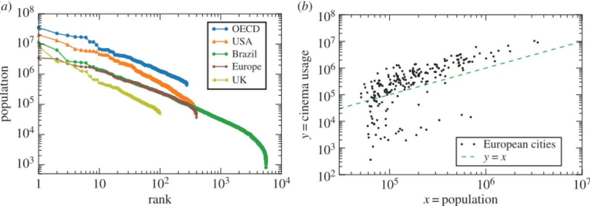
Figure 1.Example of the data and their main statistical properties. (a) The distribution of the population of the cities for the regions considered in this paper. The roughly straight line in this rank–population plot is in agreement with Zipf’s law and shows that, in most cases, the data vary over two orders of magnitude in the population (e.g. from 100 000 to 10 million inhabitants). (b) Example of the dataset analysed in our work, in which large fluctuations are clearly visible.
outputs are faster than linear inx, but claims that the populationxhas a limited explanatory factor on theper capitaratey/xof cities and function (1.1) is not better than alternative ones (see [6,18] for opposing arguments). Reference [16] focuses on the case of CO2 emissions and shows that depending on whether city boundaries or metropolitan areas are used, the value ofβchanges fromβ >1 toβ <1. This point was carefully analysed in [17] for different datasetsy. Through a careful study of different possible choices of city boundaries, the authors report that the evidence forβ=1 virtually vanishes. These results ask for a more careful statistical analysis that rigorously quantifies the evidence forβ=1 in different datasets.
In this paper, we propose a statistical framework based on a probabilistic formulation of the scaling law (1.1) that allows us to perform hypothesis testing and model comparison. In particular, we quantify the evidence in favour ofβ=1 comparing (through the Bayesian information criterion, BIC) models withβ=1 to models withβ=1. We apply this approach to 15 datasets of cities from five regions and find that the conclusions regardingβvary dramatically not only depending on the datasets, but also on assumptions of the models that go beyond (1.1). We argue that the estimation ofβis challenging and depends sensitively on the model because of the following two statistical properties of cities:
(i) the distribution of city population has heavy tails (Zipf’s law) [1,19] and
(ii) there are large and heterogeneous fluctuations ofyas a function ofx(heteroscedasticity).
Points (i) and (ii) are shown, respectively, infigure 1a,b.
The paper is organized as follows. We start by describing the problem and the datasets we use (in §2) and discussing (in §3) the limitations of the usual statistical approach based on least-squares fitting in log-scale. We then propose a probabilistic formulation together with different statistical models (in §4) and describe (in §5) how they can be compared with each other and to data. Finally, we discuss our main findings (in §6) and summarize our conclusions (in §7).
2. Data
3
rsos
.ro
yalsociet
ypublishing
.or
g
R.
Soc
.open
sc
i.
3
:1
50649
...
income, GDP), innovation (patents filed), transportation (miles travelled, number of train stations), access to culture (number of theatres, number of cinema seats, number of cinema attendances in 1 year, etc.) and health condition (AIDS infections, death by external causes). Further details are presented in appendix A.
3. Limitations of the usual statistical analysis
The following three steps summarize the usual approach used to test a nonlinear scaling in equation (1.1) (see [2–4,8,11,12,16–18] for scalings in cities and [20] for scalings in biology):
1. The parameters of equation (1.1) are chosen based on least-squares fitting in log-transformed data lny, lnx, i.e.α,βare such thatNi=1(lnαxβi −lnyi)2is minimized.
2. The quality of the fitting is quantified by the coefficient of determinationR2≡1−(
i(lnyi− lnαxβi)2)/(
i(lnyi−
jlnyj/N)2).R2close to 1 is taken as evidence of the agreement between the fit and the data.
3. The 95% confidence interval [βmin,βmax] aroundβis computed from the sum of the residuals squared andβ∈[βmin,βmax] is taken as an evidence thatβ=1.
This usual approach is appealing because of its simplicity and ease of numerical implementation. However, it contains the following assumptions and limitations that are usually ignored:
1. The parameters obtained through least-squares fitting are maximum-likelihood estimators if (i) the data points are independent and (ii) the fluctuations around the mean lny, lnα+βlnx, are Gaussian distributed in lnywith a variance independent of lnx. The value ofβobtained in the usual approach is meaningful if these assumptions hold.
2. R2does not quantify the statistical significance of the model, it quantifies the correlation between data and model (the amount of the variation in the data explained by the model). In particular,
R2close to one is not an evidence that the data are a likely outcome of the model. Below, we obtain that datasets are typically not consistent with the model underlying the usual approach. 3. The confidence interval [βmin,βmax] is a range in which the true value ofβis expected to be found
only if the model holds [21]. Therefore, in the typical case in which the data are not compatible with the model, one cannot conclude thatβ=1 based on the observation that 1∈[βmin,βmax]. Usually, in this case, bothβ=1 andβ=1 are incompatible with the data.
4. A further limitation of the usual approach is that it requires removing the datapoints withyi=0 (because it requires computing lnyi). This filtering is arbitrary, becausey=0 is usually a valid observation (e.g. cities without any patents filed).
In the study of scaling laws in biology, the underlying hypothesis and alternatives to the usual least-squares fitting have been extensively discussed [22,23]. In city data, statistical analysis beyond the usual approach was performed in [3,5,7,8,10]. It typically amounts to an analysis of the residuals lnαxβi −lnyi, e.g. a (visual) comparison of the residuals of the fit to the Gaussian distribution predicted by the model underlying the linear fit in log–log scale. The controversies regarding a nonlinear scalingβ=1 motivate us to search for an alternative statistical framework to test the scaling (1.1) beyond the usual approach with residual analysis.
4. Probabilistic models
The statistical analysis we propose is based on the likelihoodLof the data being generated by different models. Following [5], we assume that the indexy(e.g. number of patents) of a city of sizexis a random variable with probability densityP(y|x). We interpret equation (1.1) as the scaling of the expectation of
ywithx
E(y|x)=αxβ, (4.1)
4
rsos
.ro
yalsociet
ypublishing
.or
g
R.
Soc
.open
sc
i.
3
:1
50649
...
ofyaroundE(y|x) scale withx. Here, we are interested in modelsP(y|x) satisfying
V(y|x)=γE(y|x)δ. (4.2)
This choice corresponds to Taylor’s law [24]. It is motivated by its ubiquitous appearance in complex systems [25], where typicallyδ∈[1, 2], and by previous analysis of city data that reported non-trivial fluctuations [8,26,27]. The fluctuations in our models aim to effectively describe the combination of different effects, such as the variability in human activity and imprecisions on data gathering. In principle, these effects can be explicitly included in our framework by considering distinct models for each of them.
Below, we specify different modelsP(y|x) compatible with equations (4.1) and (4.2). We consider two classes of models. In the first class, which we call city models, we a priorichoose a parametric form forP(y|x), and we use equations (4.1) and (4.2) to fix the free parameters. In the second class, which we call person models, we derive P(y|x) from a generative process for the assignment of y
to people that is compatible with equations (4.1) and (4.2). In both cases, the likelihood L of the model is written as a function of the data{(xi,yi)}i=1,...,N and at most four free parameters (α,β,γ andδ).
4.1. City models
In this class of models, we assume that each data point yi is an independent realization from the conditional distributionP(y|xi) and therefore the log-likelihood can be written as
lnL≡lnP(y1,. . .,yN|x1,. . .,xN)= N
i=1
lnP(yi|xi). (4.3)
In order to explore how the choice ofP(y|x) affects the outcome of the statistical analysis, we consider two different continuous distributions (Gaussian and lognormal).1
4.1.1. Gaussian fluctuations
Here, we consider that P(y|x) is given by a Gaussian distribution with parameters μN(x) and σN(x)
P(y|x)=√ 1 2πσN(x)e
−(y−μN(x))2/2σ2
N(x). (4.4)
The relations (4.1) and (4.2) are fulfilled choosing the parameters as
μN(x)=αxβ
and σN2(x)=γ(αxβ)δ.
⎫ ⎬
⎭ (4.5)
The log-likelihood (4.3) is given by
lnL= N
i=1 −ln
σN(xi)
√
2π−(yi−μN(xi))2 2σ2
N(xi)
. (4.6)
This model hasP(y≤0|x)>0 and therefore observations with yi≤0 can be accounted for. For the observables considered here,y=0 is a valid observation buty<0 is not.
We consider two cases:
Fixedδ=1. This is the typical fluctuation scaling found whenyi is the result of a sum of random variables [25].
Freeδ∈[1, 2].The general functional form that fulfils equation (4.2). We excludeδ >2, because, in this case, the probabilityP(y<0|x) of negative values (not feasible for most observablesy) remains large for largex.
5
rsos
.ro
yalsociet
ypublishing
.or
g
R.
Soc
.open
sc
i.
3
:1
50649
...
4.1.2. Lognormal fluctuations
Here, we consider thatP(y|x) is given by a lognormal distribution with parametersμLN(x) andσLN(x):
P(y|x)=√ 1 2πσLN(x)
1
ye
−(lny−μLN(x))2/2σ2
LN(x). (4.7)
The relations (4.1) and (4.2) are fulfilled choosing the parameters as (see appendix B)
μLN(x)=lnα+βlnx−12σLN2 (x) and σLN2 (x)=ln[1+γ(αxβ)δ−2].
⎫ ⎬
⎭ (4.8)
The log-likelihood (4.3) is given by
lnL= N
i=1
−ln(σLN(xi) √
2π)−lnyi−
(ln(yi)−μLN(xi))2 2σ2
LN(xi)
. (4.9)
This model hasP(y≤0|x)=0 and therefore observations withyi≤0 cannot be accounted for. We again consider two cases:
Fixed δ=2. This scaling is obtained when yi is the product of independent random variables. Furthermore, σLN2 (x) and the fluctuations of lnyare independent of xand therefore the maximum-likelihood estimation ofβcoincides with the estimation obtained with minimum least-squares for lny, as discussed in §3.
Freeδ∈[1, 3].The general functional form that fulfils equation (4.2).
4.2. Person model
The starting point for this class of models is the natural interpretation of equation (1.1) that people’s efficiency (or consumption) scales with the size of the city they are living in. This motivates us to consider a generative process in which tokens (e.g. a patent, a dollar of GDP, a mile of road) are produced or consumed by (assigned to) individual persons, in the same spirit as in [12,14]. Specifically, considerj=
1,. . .,Mpersons living ini=1,. . .,Ncities, on which the population of the cityiis given byxisuch that
N
i xi=M. Consider also that there is a total ofk=1,. . .,Ytokens that are randomly assigned to theM persons. A super-linear (sublinear) scaling suggests that a token is more likely to be assigned to someone living in a more (less) populous city. In this spirit, we assume that the probability that a token is assigned to personjdepends only on the populationx(j)of the city where personjlives as
p(j)=x
β−1 (j)
Z(β), (4.10)
whereZ(β) is the normalization constant, i.e.Z(β)=Mj x(βj−)1. Forβ=1,p(j)=1/Mand each person is equally likely to be assigned a token (independently of the population of its city). Equation (4.10) is a microscopic model, and we are now interested in the macroscopic behaviour of the city: the probability that a cityigetsyitokens, given that its population isxi. Assuming that besides their city, individuals are indistinguishable, the probabilityp(i) that a token is assigned to a cityiis given by a sum ofp(j) over personsjon cityi, which contains exactlyxiterms. Because x(j)=xi when the personjlives in cityi, represented byj∈i, we obtain
p(i)= j∈i
xβ(j−)1 Z(β)=
xβi
Z(β). (4.11)
The probability of observingyitokens in each city of sizexiis a multinomial distribution
P(y1,. . .,yN|x1,. . .,xN)=Y! N
i=1 1
yi!
xβi Z(β)
yi
. (4.12)
Thus, the likelihood can be written as a function of the observed quantities (xi,yi) as
lnL≡lnP(y1,. . .,yN|x1,. . .,xN)=lnY!− N
i=1
ln(yi!)+ N
i=1
yiln
xβi Z(β)
6
rsos
.ro
yalsociet
ypublishing
.or
g
R.
Soc
.open
sc
i.
3
:1
50649
...
The scaling of the average and variance ofy, i.e. equations (4.1), (4.2), is recovered as
E(yi|xi)=Yp(i)=
Y Zβx
β
i
and V(yi|xi)=Yp(i)[1−p(i)]≈Yp(i)=E(yi|xi), ⎫ ⎪ ⎬ ⎪
⎭ (4.14)
where we identify thatα=Y/Z(β),γ=1 andδ=1. Foryi 1, this model coincides with the city model with normal fluctuations and the latter choice of parameters. Note that the fluctuations of this model account only for fluctuations of the assignment, and neglects potential fluctuations of measurement imprecisions.
5. Results
In this section, we compare the models presented above against our 15 datasets. In particular, we address the following questions whose answers are summarized intable 1:
1. What is the estimated value ofβ?
For each model, we calculate the parameters (α,β,γ,δ) that maximizeL(see appendix C for details). Intable 1, we reportβ.
2. What is the error bar b around the estimatedβ?
We estimatebusing bootstrapping with replacement (see appendix D for details). Intable 1,bis shown in parentheses. The interval [β−b,β+b] can be interpreted as the 95% confidence interval ofβwhen the model is not rejected. Otherwise, it can be interpreted as the robustness of the estimatedβagainst fluctuations in the data (cross validation).
Hypothesis testing
3. Are the data compatible with the model?
We test the hypothesis that the data were generated by the model. Specifically, for each model, we compute ap-value that quantifies (i) whether the fluctuations in the data are compatible with the expected fluctuations from the model and (ii) whether the residuals are uncorrelated (see appendix E for details). In the case the model is not rejected, i.e.p-value>0.05, the corresponding entry intable 1
is marked with an asterisk.
Model comparison
4. What is the statistical evidence forβ=1?
We quantify the evidence forβ=1 by comparing the maximum-likelihoodLof each model with the corresponding model where we fixβ=1. We account for the different number of free parameters (e.g. to avoid overfitting) by using the BIC, BIC= −2 lnL+klnN, wherekis the number of free parameters andN the number of observations (see appendix F for details). The difference in the BIC,BIC≡ BICβ=1−BICβindicates whether the model withβ=1 provides a sufficiently better description of the data. From this we infer that, for (i)BIC<0 the model with fixedβ=1 (linear scaling) is better, (ii) 0≤BIC<6 the evidence forβ=1 is inconclusive, and (iii)BIC≥6 the model withβ=1 (nonlinear scaling) is better. Intable 1, these results are indicated by the symbols (i)→(linear), (ii) open circle (inconclusive), or (iii)(sublinear) or(super-linear).
5. What is the statistical evidence for fluctuation scaling (Taylor’s law)?
We quantify the evidence forδ=1 (δ=2), i.e. non-trivial scaling in the fluctuations in equation (4.2), in the models of cities with Gaussian (lognormal) noise. Within each class, we calculateBIC≡BICδ∗− BICδ, where we compare the BICs of the model where (i)δis fixed (BICδ∗) and (ii) whereδis a free parameter (BICδ). In case ofBIC>0, the model withδas a free parameter (non-trivial fluctuation scaling) provides a better description of the data (see appendix F for details). Intable 1, the entry for the selected model is highlighted with a grey background.
6. Which model best describes the data?
7
rsos
.ro
yalsociet
ypublishing
.or
g
R.
Soc
.open
sc
i.
3
:1
50649
...
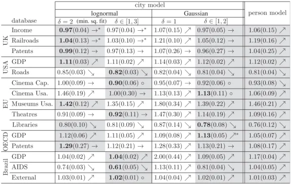
Table 1.Summary of the application of our statistical framework to 15 different databases and five models. The entries in the table represent the scaling exponentβ. The value obtained through least-squares fitting in log-scale coincides with the value reported in the first column. The error bars were computed with bootstrap. The asterisk indicates that the model has ap-value higher than 0.05. If the differenceBIC between the BIC of each model with the same model with a fixedβ=1 is below 0, the model is linear (→), between zero and six is inconclusive (open circle) and higher than six (strong evidence) is super-linear ()/sublinear (). The models were also compared between each other using the respective BICs within the same noise model (grey background has lower BIC) and between all others (bold text indicates the model with the lowest BIC).
lognormal Gaussian
(min. sq. fit)
6. Discussion
In this section, we interpret the outcome of the statistical analysis summarized intable 1. We focus on specific findings and their significance to the problem of scaling in cities.
6.1. Data are almost never compatible with the proposed models
In almost all cases, the data are not a typical outcome of any of the five proposed models, leading to a rejection of the models (p-value<0.05). The only exceptions (marked by an asterisk intable 1) are the two lognormal models in UK-income and UK-train stations, and the Gaussian model with freeδfor OECD-GDP. There are several possible reasons for the widespread rejection of the models: fluctuations of the data may differ from the fluctuationsP(y|x) of the models (e.g. measurement errors are not correctly accounted for by P(y|x)); the observations are not independent (e.g. there are correlations between residuals and city size); different scalings are observed for small and large cities (as discussed in [28] andfigure 3).
The rejections of the models considered here are a consequence of their strong simplifying hypothesis and show that the development of better models is needed in order to understand the observations and clarify the existence of the nonlinear scaling (1.1). It shows also that the estimated confidence interval cannot be used (in the rejected models) to discard a linear scalingβ=1 [21]. Still, the widespread rejection of models does not imply that the nonlinear scaling (1.1) is rejected altogether because it is possible that the data are well described by another (unknown) model consistent with equation (4.1) but different from the ones considered here, e.g. having different fluctuations inP(y|x). These alternative models can have different fluctuation relations or can account for the known (e.g. spatial [3]) correlations in the data. In particular, the generative process underlying the person model could be generalized to account for other effects beyond city-size population (e.g. individuals could be segmented by income).
8
rsos
.ro
yalsociet
ypublishing
.or
g
R.
Soc
.open
sc
i.
3
:1
50649
...
y
EU-cinema usage EU-theatres
yµ x yµ x
103
102
104 105
106
107
108
1 103
102
10
d= 2
freed freefreedd
104 105 106 107
x 10
4 105 106 107
x
(b) (a)
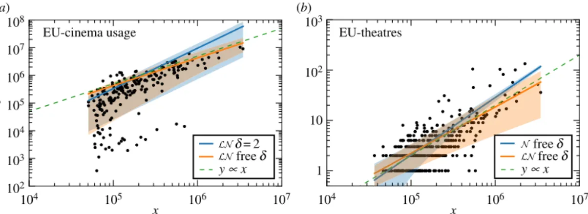
Figure 2.Effect of fluctuations on the estimation ofβ. (a) In the ‘EU cinema usage’ database, the lognormal model withδ=2 yields β=1.46, whereas freeδyieldsβ=1.00. (b) In the ‘EU theatres’ database, the lognormal with freeδyieldsβ=0.92, a lower value thanβ=1.14 obtained in the Gaussian model with freeδ. Shaded areas represent the 68th percentile (±1 s.d.) ofP(y|x).
in the next sections are mostly based on model comparison: we analyse which model and parameters best describe the data, with particular interest in the parameterβ.
6.2. Different datasets are best described by different models
There is no single model that best describes all databases (the bold value intable 1appears in different rows). A systematic observation on the 15 datasets is that the person model and the Gaussian model with fixedδare never the best ones. This indicates that the fluctuations in the (large) cities are much larger than predicted by the scalingδ=1 used in both models. For the other models, there are databases in which they are the best models: the lognormal with fixedδ=2 is the best model in the three UK cases and for USA-GDP; the lognormal model with freeδis the best model for USA-roads and EU-cinema capacity; and the Gaussian model with freeδis the best for EU-cinema usage, OECD-GDP and EU-libraries. The inclusion of the additional parameterδin the lognormal model, related to Taylor’s law in equation (4.2), is considered beneficial in eight out of the 15 cases (shaded grey regions in the two first rows oftable 1). Altogether, these results show that the model underlying the usual approach (lognormal with fixedδ) is often not the best model.
6.3. The estimated
β
depends on the model
Models consistent with the average scaling (4.1), but that have different assumptions regarding the fluctuations, can lead to different estimations ofβ. Consider the case of EU-cinema attendance. The value estimated from the lognormal model with fixedδisβ=1.46±0.19. It coincides with the usual approach (least-square fitting) and suggests a super-linear relation between the number of cinema visitors and the population of cities. However, if we allow for a different fluctuation scaling as in the lognormal model with freeδ, a model that is preferred according to our BIC test, we obtain that β=1.00±0.30, i.e. a linear scaling. Conflicting conclusions are observed also in the EU-theatres database. The data and fittings for these two cases are shown infigure 2. Visual inspection of the graph can be misleading because of the log-scale and the different density of points, and shows the need for more careful (quantitative) statistical analysis. Altogether, the variation ofβ across different models shows that conclusions regardingβ(e.g.β=1) cannot be done independently from the analysis of the fluctuations. Considering also that different models are preferred for different databases (previous point), this confirms the practical importance of going beyond the usual approach (least-square fitting) both in terms of methods and models, as proposed in this paper.
6.4. Models are dominated either by the small or the large cities
9
rsos
.ro
yalsociet
ypublishing
.or
g
R.
Soc
.open
sc
i.
3
:1
50649
...
1 10 102
103
104
1.0
103 104 105 106 107
0.8 0.6 0.4 0.2 0
80% of the cities
75% of the population
city model person model running mean
x, population
fraction
<
xy
, Brazil-AIDS
(b) (a)
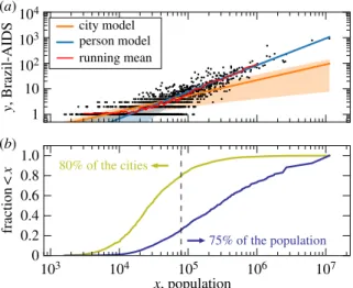
Figure 3.Comparison of the model of cities and persons. (a) Scaling of the city model, i.e. lognormal with freeδ, and the person model (solid lines) for the data of Brazil-AIDS (dots). While the city model captures a sublinear scaling present in small citiesβ=0.61, the person model describes the roughly linear scalingβ=1.04 of large cities. Shaded areas represent 1 s.d. The running mean (red line) is the average (x,y) over 50 datapoints,{x,y}, in a sliding window over the data ordered inx. (b) Cumulative distribution of heavy-tailed distribution of city sizes in terms of cities and persons, i.e. the fraction of (i) cities of size≤x(city model) and (ii) the population in cities of size≤x.
to most points, i.e. it weights a village as much as a million-size city. The fit will be thus dominated by the large number of small cities. The disadvantage of this is that, even if the model describes well most cities, it may fail to describe the behaviour of most of the population. Our person model addresses this issue by giving the same weight to each person, leading to the problem of describing most people but potentially not most cities. To see this, consider the example of the 5565 Brazilian cities. Half of the Brazilian population lives in the 201 largest cities (3.6% of cities); yet, 50% of smallest cities account for only 8.2% of the total population. This is a direct consequence of the heavy-tailed distribution of city sizes, which holds in all our databases (figure 1a). Our city models with freeδin equation (4.2) allow cases beyond the least-squares fitting (δ=2) and person model (δ=1). The exponentδ controls how the variance ofP(y|x) grows withx. A small variance for largex, obtained for smallδ, will force the fitted curve (average) to pass close to the points of large cities. The weight of the large cities is inversely proportional toδ.
The general considerations above explain a great extent of the variation of β across the models observed intable 1. The values obtained for the Gaussian model withδ=1 and the person model are dominated by large cities, in the lognormalδ=2 case, they are dominated by small cities, whereas for the freeδmodels, it depends on which bestδis obtained. In the Brazil-AIDS datasetδ≥2 andβis dominated by the small cities (δ=2 in the Gaussian model andδ=2.79 in the lognormal model). Accordingly, the values ofβfor these two models in the second to last row oftable 1areβ1 in agreement with the lognormal withδ=2 case and in contrast with the Gaussianδ=1 and person model which haveβ >1 and are dominated by the large cities.Figure 3shows the results for this dataset and emphasizes how different models describe different city sizes. The same reasoning also explains the values ofβof other databases reported intable 1(e.g. all UK cases).
10
rsos
.ro
yalsociet
ypublishing
.or
g
R.
Soc
.open
sc
i.
3
:1
50649
...
plot, this is only justified if the scaling (1.1) is interpreted as being valid only for large cities. The latter interpretation limits the relevance of the scaling because it becomes limited to a small fraction of the total cities.
6.5. Is the scaling nonlinear?
New answers to this central question emerge from the results of our paper (summarized intable 1). In three of the 15 cases, we found models which are reasonably compatible with the data, and we can base our conclusions on these models, i.e. on the obtainedβand on the model comparison with the case β=1 (arrows→,↑,intable 1). This leads to the conclusion that the UK-income and UK-train stations show linear and OECD-GDP shows super-linear scaling. In the remaining 12 cases, conclusions are based solely on model comparison, and we feel more confident to give an answer to this question only when the same conclusion is obtained for models with different fluctuations (i.e. we compare the conclusions obtained in the best model with lognormal and Gaussian fluctuations). We find such an agreement in eight of the 12 cases, so that the scalings are: UK-patents and OECD-patents are linear; USA-GDP, EU-museum usage and Brazil-GDP are super-linear; USA-roads, EU-libraries and Brazil-AIDS are sublinear. For the remaining four cases, our analysis isinconclusiveon the question of linear or nonlinear scaling. Two reasons can lead to this conclusion. The first is that the nonlinear scaling qualitatively changes fromβ <1 toβ >1 depending on the assumptions of the fluctuations (e.g. EU N. theatres). The second reason is that in one of the best models there is no sufficient statistical evidence forβ=1 (marked by an open circle intable 1, EU-cinema capacity, EU-cinema usage and Brazil-external). One interesting case falling in this second reason is EU-cinema usage, for which both the lognormal with fixedδand the best model (Gaussian with freeδ) yieldβ >1. We still consider this case inconclusive, because the best model, despite showingβ=1.13±0.11, only marginally improves (0<BIC<6) upon the model with β=1. In this case, additional data are required in order to increase the statistical evidence in favour of either situation. The possibility of reaching an inconclusive answer shows the advantage of the statistical framework proposed here. In summary, in 15 datasets, we found four linear, four super-linear and three sublinear scalings.
7. Conclusion
In summary, we investigated the existence of non-trivialβ=1 scalings in city datasets. We introduced five different models, showed how to compare them and how to estimateβ, and finally tested our methods and models in 15 different datasets. We found that in most cases models are rejected by the data and conclusions can be based only on the comparison between the descriptive power of the different models considered here. Moreover, we found that models which differ only in their assumptions on the fluctuations can lead to different estimations of the scaling exponentβ. In extreme cases, even the conclusion on whether a city index scales linearlyβ=1 or nonlinearlyβ=1 with city population depends on assumptions on the fluctuations. A further factor contributing to the large variability ofβ is the broad city-size distribution that makes models to be dominated either by small or by large cities. In particular, these results show that the usual approach based on least-square fitting is not sufficient to conclude on the existence of nonlinear scaling.
Recent works focused on developing generative models of urban formation that explain nonlinear scalings [10–14]. Our finding that most models are rejected by the data confirms the need for such improved models. The significance of our results on models with different fluctuations is that they show that the estimation ofβand the development of generative models cannot be done as separate steps. Instead, it is essential to consider the predicted fluctuations not only in the validation of the model, but also in the estimation ofβ. Finally, the methods and models used in our paper can be applied to investigate scaling laws beyond cities [20,23].
Data accessibility. Datasets and code used in this paper are available athttp://dx.doi.org/10.5281/zenodo.49367. Authors’ contributions. All the authors were involved in the design of the project, data analysis and the preparation of the manuscript.
Competing interests. The authors declare that they have no competing interests.
Funding. J.C.L. acknowledges support from the Portuguese Foundation for Science and Technology (FCT), scholarship SFRH/BD/90050/2012.
11
rsos
.ro
yalsociet
ypublishing
.or
g
R.
Soc
.open
sc
i.
3
:1
50649
...
Appendix A. Databases
We used 15 datasets from five different databases. In each database (UK, USA, EU, OECD and Brazil), the same citiesxiwere used, and the different datasets are different indexesy. Some of our models cannot consideryi≤0. In order to allow for a comparison across all models, we ignoredyi≤0 in all cases, and below we report the numberNof casesyi>0 in each dataset.
— UK: this database corresponds to fig. 5b of [17], was provided by the authors of that paper, includes the aggregation of population in cities proposed in that paper, and corresponds to the period 2000–2011.
— Income:N=100, total income (weekly). — Train stations:N=97, number of train stations. — Patents:N=93, number of patents filed in the period.
— USA: this database corresponds to metropolitan areas of the USA (GDP) and urban areas (roads) in 2013. It was constructed from three different sources: the population was provided by US Census Bureau [29]; the GDP was provided by the US Bureau of Economics Analysis of the Department of Commerce [30]; and the miles of roads was provided by the US Federal Administration of Highways of the Department of Transportation (table HM-71) [31]. Similar data were used in [12].
— GDP:N=381, gross domestic product of metropolitan areas. — Roads:N=459, length (in miles) of roads of urban areas.
— EU: this database is provided by Eurostat [32]. It contains population and different indexes related to culture in European cities in the year 2011.
— Cinema capacity:N=418, total number of seats of cinemas. — Cinema usage:N=221, attendance of cinemas in the year. — Museums usage:N=443, attendance of museums in the year. — Theatres:N=398, number of theatres.
— Libraries:N=597, number of public libraries.
— OECD: this database contains indexes of cities from the Organization for Economic Co-operation and Development in the years 2000–2012 [33].
— GDP:N=275, gross domestic product in 2010. — Patents:N=218, number of patents filed in 2008.
— Brazil: this database contains different indexes of all municipalities of Brazil. The data are from the year 2010 and are provided by Brazil’s Health Ministry (Brazilian Health Ministry. July 2015; population corresponds to census data).
— GDP:N=5565, gross domestic product. — AIDS:N=1812, number of deaths by AIDS.
— External:N=5286, number of deaths by external causes.
All the above databases are provided athttp://dx.doi.org/10.5281/zenodo.49367.
Appendix B. Taylor’s law in lognormal
Here, we express the parameters of the lognormal distribution,μLN(x) andσLN2 (x), as a function of the parameters of the scaling laws
E(y|x)=αxβ (4.1) and
V(y|x)=γE(x)δ, (4.2) α,β,γ andδ. Noting that the expectation and the variance of the lognormal distribution, equation (4.7), are given by
E(y|x)=eμLN(x)+σLN2 (x)/2 (B 1)
and
12
rsos
.ro
yalsociet
ypublishing
.or
g
R.
Soc
.open
sc
i.
3
:1
50649
...
we find a unique solution forμLN(x) andσLN2 (x) by comparing with equations (4.1) and (4.2): μLN(x)=lnα+βlnx− 12σLN2 (x)
and σLN2 (x)=ln[1+γ(αxβ)δ−2]. ⎫ ⎬
⎭ (4.8)
Appendix C. Maximization of the likelihood
The maximization of the likelihood is performed by minimizing minus the log-likelihood, using the algorithm ‘L-BFGS-B’ [34], whose implementation can be found on the Python package SciPy [35], and the details can be found athttp://dx.doi.org/10.5281/zenodo.49367. Given that the minimization algorithm can converge to a local minimum, our procedure repeats the optimization 512 times, each with random initial parameters, and selects the lowest. We confirmed that increasing from 256 to 512 samples did not change the computed minima, an indication that the algorithm found the global one.
Appendix D. Computation of the error estimates
The error estimates were computed using bootstrap [36]. The method consists of samplingNpairs (xi,yi) with replacement from the set ofN available data points, and repeating the maximization procedure outlined in the previous section for each set. This procedure (sampling+maximization) was repeated 100 times for each combination (model, dataset) and the error estimates were computed as the standard deviation of the distances from the measured parameters to the estimated parameter from the true dataset. We confirmed that the bootstrap error estimates for the lognormal fixed-δcase are within 1% equal to the values of the least-square fit.
Appendix E. Computation of the
p
-value
The computation of thep-value was done by defining a statistic that tests the hypothesis used in each model; in the case of the lognormal and normal models these are (i) data are independent and (ii) the data are compatible with the model. We used a statistic based on the D’AgostinoK2test [37] (over lnyory, respectively) that computes the deviations from 0 of the empirical kurtosis and skewness; the test consist of comparing it with the fluctuations expected from a finite-size sample from the (null) model. In detail, we compute two statistics,ZsandZkfor the kurtosis and skewness, respectively. Each of them has aχ12 distribution under the null hypothesis, so the sumK2=Z2
s+Z2khas aχ22distribution (with 2 degrees of freedom). Because this test does not test independence of the samples, we include in the test statistic the Spearman’s rank correlation [38] of the residuals of the fit,ZS (also distributed as aχ12) because if the residuals are correlated, the data are not independent. Thep-value is thus computed by measuring how extremeK2=Z2s+Zk2+Z2Sis in theχ32distribution (with 3 degrees of freedom). The implementation of this is available athttp://dx.doi.org/10.5281/zenodo.49367.
In the population model, the calculation of thep-value must be different, because the variance is not being left as a free parameter, so we take a moreclassicalapproach. Thep-value is computed by measuring how extreme is the difference between the data and its fit with respect to the difference between a sample from the model and its fit. In practice, we use aχ2statistic to measure the distance between two sets of points{yi}i (data) and{mi}i (the model),χ2=
i(yi−mi)2/yi. Then, we generate from the model 200 different samples. For each of these samples, we compute theχ2between the sample values and their fits. Finally, we compute thep-value as the fraction of samples whoseχ2 is bigger than the one that belongs to the real data. Note that this statistic is not taking into account independence of the residuals (if we consider the multinomial distribution as the null model, then they should not be independent) or normality in the strict sense, so this test is more permissive than the previous.
Appendix F. Model comparison using Bayesian information criterion
We compare two modelsm=1, 2 by calculating the BIC [39], BICm≡ −2 lnLm+kmlnN, whereNis the number of data points (observations),Lmis the maximum-likelihood of the model, andkmis the number of estimated (free) parameters of the model. In this approach, the model with a lower value for the BIC gives a better description of the data.
13
rsos
.ro
yalsociet
ypublishing
.or
g
R.
Soc
.open
sc
i.
3
:1
50649
...probability of the data given the model. It can be shown [36] that this quantity can be approximated by
B12≈eBIC/2, (F 1)
whereBIC≡BIC2−BIC1is the difference of the respective BICs. Thus, if BIC1<BIC2, it follows that
B12>1, i.e. that model 1 provides a better description of the data than model 2. Regarding the decision about nonlinear scaling, i.e.β=1, we require thatBIC≡BICβ=1−BICβ≥6 (see main text), in line with [40], where it is suggested that this implies strong or very strong evidence for a model withβ=1. This corresponds toB12≥e3≈20.08, i.e. it is at least 20 times more likely that the data come from a model withβ=1.
References
1. Batty M. 2013The new science of cities. Cambridge,
MA: MIT Press.
2. Bettencourt LMA, Lobo J, Helbing D, Kuhnert C,
West GB. 2007 Growth, innovation, scaling, and the pace of life in cities.Proc. Natl Acad. Sci. USA104,
7301–7306. (doi:10.1073/pnas.0610172104)
3. Bettencourt LMA, Lobo J, Strumsky D, West GB. 2010
Urban scaling and its deviations: revealing the structure of wealth, innovation and crime across
cities.PLoS ONE5, e13541. (doi:10.1371/journal.
pone.0013541)
4. Arbesman S, Christakis NA. 2011 Scaling of prosocial
behavior in cities.Physica A, Stat. Mech. Appl.
390, 2155–2159. (doi:10.1016/j.physa.2011.
02.013)
5. Gomez-Lievano A, Youn H, Bettencourt LMA. 2012
The statistics of urban scaling and their connection
to Zipf’s law.PLoS ONE7, e40393. (doi:10.1371/
journal.pone.0040393)
6. Bettencourt LMA, Lobo J, Youn H. 2013 The hypothesis of urban scaling: formalization,
implications and challenges. (http://arxiv.org/
abs/1301.5919)
7. Alves LGA, Ribeiro HV, Lenzi EK, Mendes RS. 2013
Distance to the scaling law: a useful approach for unveiling relationships between crime and urban
metrics.PLoS ONE8, e69580. (doi:10.1371/journal.
pone.0069580)
8. Nomaler Ö, Frenken K, Heimeriks G. 2014 On scaling of scientific knowledge production in U.S.
metropolitan areas.PLoS ONE9, e110805.
(doi:10.1371/journal.pone.0110805) 9. Oliveira EA, Andrade Jr JS, Makse HA. 2014 Large
cities are less green.Sci. Rep.4, 4235. (doi:10.1038/ srep04235)
10. Samaniego H, Moses ME. 2008 Cities as organisms:
allometric scaling of urban road networks.J.
Transport Land Use1, 21–39. (doi:10.5198/jtlu.
v1i1.29)
11. Um J, Son S-W, Lee S-I, Jeong H, Kim BJ. 2009 Scaling laws between population and facility
densities.Proc. Natl Acad. Sci. USA106,
14 236–14 240. (doi:10.1073/pnas.0901898106)
12. Bettencourt LMA. 2013 The origins of scaling in
cities.Science340, 1438–1441. (doi:10.1126/science.
1235823)
13. Pan W, Ghoshal G, Krumme C, Cebrian M, Pentland A. 2013 Urban characteristics attributable to
density-driven tie formation.Nat. Commun.4, 1961.
(doi:10.1038/ncomms2961)
14. Yakubo K, Saijo Y, Korošak D. 2014 Superlinear and sublinear urban scaling in geographical networks
modeling cities.Phys. Rev. E90, 022803.
(doi:10.1103/PhysRevE.90.022803) 15. Shalizi CR. 2011 Scaling and hierarchy in urban
economies. (http://arxiv.org/abs/1102.4101)
16. Louf R, Barthelemy M. 2014 Scaling: lost in the
smog.Environ. Plan. B: Plan. Des.41, 767–769.
(doi:10.1068/b4105c)
17. Arcaute E, Hatna E, Ferguson P, Youn H, Johansson A, Batty M. 2015 Constructing cities, deconstructing scaling laws.J. R. Soc. Interface12, 20140745. (doi:10.1098/rsif.2014.0745)
18. Bettencourt LMA, Lobo J. 2015 Urban scaling in
Europe. (http://arxiv.org/abs/1510.00902)
19. Rybski D. 2013 Auerbach’s legacy.Environ. Plan. A
45, 1266–1268. (doi:10.1068/a4678)
20. Savage VM, Gillooly JF, Woodruff WH, West GB, Allen AP, Enquist BJ, Brown JH. 2004 The predominance of quarter-power scaling in biology.
Funct. Ecol.18, 257–282. (doi:10.1111/j.0269-8463.
2004.00856.x)
21. Thulin M. 2014 On confidence intervals and two-sided hypothesis testing. PhD thesis, Uppsala University, Sweden.
22. Zar JH. 1968 Calculation and miscalculation of the allometric equation as a model in biological data.
Bioscience18, 1118–1120. (doi:10.2307/1294589)
23. Warton DI, Wright IJ, Falster DS, Westoby M. 2006
Bivariate line-fitting methods for allometry.Biol.
Rev.81, 259–291. (doi:10.1017/S1464793106007007)
24. Taylor LR. 1961 Aggregation, variance and the mean.
Nature189, 732–735. (doi:10.1038/189732a0)
25. Eisler Z, Bartos I, Kertész J. 2008 Fluctuation scaling
in complex systems: Taylor’s law and beyond.Adv.
Phys.57, 89–142. (doi:10.1080/00018730801893043)
26. Hanley QS, Khatun S, Yosef A, Dyer R-M. 2014
Fluctuation scaling, Taylor’s law, and crime.PLoS
ONE9, e109004. (doi:10.1371/journal.pone.0109004)
27. Greig A, Dewhurst J, Horner M. 2015 An application of Taylor’s power law to measure overdispersion of
the unemployed in English labor markets.Geogr.
Anal.47, 121–133. (doi:10.1111/gean.12046)
28. Hanley QS, Lewis D, Ribeiro HV. 2016 Rural to urban population density scaling of crime and property transactions in English and Welsh parliamentary
constituencies.PLoS ONE11, e0149546. (doi:10.1371/
journal.pone.0149546)
29. US Census Bureau. 2014 Seewww.census.gov/
popest/data/metro/totals/2014/. 30. US Bureau of Economics Analysis. 2015 See
www.bea. gov/itable/index_regional.cfm. 31. US Department of Transportation. 2015 See
www.fhwa.dot.gov/policyinformation/ statistics/2013/.
32. Eurostat. 2015 Seehttp://ec.europa.eu/eurostat/
web/cities/data/database.
33. OECD. 2015 See
http://dx.doi.org/10.1787/data-00531-en.
34. Byrd RH, Lu P, Nocedal J, Zhu C. 1995 A limited memory algorithm for bound constrained
optimization.SIAM J. Sci. Comput.16, 1190–1208.
(doi:10.1137/0916069)
35. Jones E, Oliphant T, Peterson P. 2001 SciPy: open
source scientific tools for Python. Seehttp://www.
scipy.org.
36. Hastie T, Tibshirani R, Friedman. J. 2009The
elements of statistical learning, 2nd edn. Springer
Series in Statistics. New York, NY: Springer.
37. D’Agostino RB. 1986Goodness-of-fit-techniques.
New York, NY: Marcel Dekker.
38. Kendall MG 1970Rank correlation methods, 4th edn.
London, UK: Griffin.
39. Schwarz G. 1978 Estimating the dimension of a
model.Ann. Stat.6, 461–464. (doi:10.1214/aos/
1176344136)
40. Kass RE, Raftery AE. 1995 Bayes factors.J. Am. Stat.
Assoc.90, 773–795. (doi:10.1080/01621459.1995.