ESTIMATING THE IMPACTS OF INTERVENTIONS ON NON-AIDS RISK FACTORS IN OBSERVATIONAL HIV COHORTS
Tiffany Lyn Breger
A dissertation submitted to the faculty at the University of North Carolina at Chapel Hill in partial fulfillment of the requirements for the degree of Doctor of Philosophy in the Department of Epidemiology
in the Gillings School of Global Public Health.
Chapel Hill 2020
ABSTRACT
Tiffany Lyn Breger: Estimating the Impacts of Interventions on Non-AIDS Risk Factors in Observational HIV Cohorts
(Under the direction of Stephen R. Cole)
Non-AIDS risk factors contribute to persisting health disparities between people with HIV and the general population in the current era of effective combination antiretroviral therapy (ART). However, the optimal combination of interventions used in conjunction with ART to improve long-term outcomes remains unclear. In Aim 1, we used the parametric g-computation estimator to estimate the effects of combined interventions on non-AIDS risk factors on the risk of all-cause mortality among 1016 ART-naïve women enrolled in the Women’s Interagency HIV Study (WIHS) between 1998 and 2017. Modeled interventions on alcohol and smoking combined with prompt initiation of modern ART decreased the 8-year risk of mortality compared to intervening solely on ART. Strategies that eliminated these non-AIDS risk factors achieved greater improvements in survival than strategies that reduced the prevalence of alcohol and smoking based on the expected efficacy of existing, real-world interventions.
While modern ART has transformed the prognosis of HIV to a manageable chronic condition, non-AIDS risk factors remain significant contributors to early mortality. Our results suggest that
interventions targeting alcohol and smoking may further reduce the risk of mortality. Achieving optimal health outcomes, however, will require more efficacious interventions as well as evaluation of
To my mentors,
both professional and personal, who helped me construct a wider lens
ACKNOWLEDGEMENTS
Writing this acknowledgement section of my dissertation is both the easiest and most difficult task of this whole process. While I was fortunate enough to receive an incredible amount of support from numerous individuals, it is not possible to fully convey the impact they have had on the completion of this body of work and my development as a scholar.
First, I would like to thank my committee. Steve Cole has been everything one could hope for in a mentor. He has challenged me, encouraged me, and advocated for me, and pushed me to think more deeply, question more often, and seek more opportunities to learn. One of the greatest gifts he has given me is teaching me how to learn. Jess Edwards has been nothing short of a rock star. My first encounter with Jess was when I attended her dissertation defense when I was visiting UNC as a prospective student. That became my vision of what doctoral level work looked like, and with no other reference or
knowledge of what an extraordinary epidemiologist Jess was, I had no idea she had set the bar so high. In the four years I have been lucky enough to work with her, Jess has taught me to pursue creativity, think outside of the box, and never set limits on what is possible for myself. She has provided me with
the research questions most pressing for people with HIV. She has helped me become a better
communicator to clinical and health policy audiences and has kept me focused on the work that matters. I am also appreciative of the funding I received throughout my doctoral training. The research for my dissertation papers was supported by the National Institutes of Health through the UNC WIHS (U01-AI-103390 PI: Adaora Adimora) and the Office of the Director and the Eunice Kennedy Shriver National Institute of Child Health & Human Development (DP2-HD-084070 PI: Daniel Westreich). Throughout my time at UNC, I was also fortunate to receive support from a UNC Center for AIDS Research supplement (PI: Jessie Edwards), the National Institutes of Health through the National Institute of Mental Health (R01-MH1000970 PI: Brian Pence; R01-MH087118-02 PI: Audrey Pettifor), and the African Studies Center as part of the Foreign Language and Area Studies Fellowship. I am incredibly fortunate to have always had a funding source and principal investigators that provided protected time to learn and advance my research interests.
My professors at UNC provided me with a solid foundation in this field. I especially thank those who were with me for the methods sequence – Steve Marshall, Daniel Westreich, Charlie Poole, Christy Avery, Brian Pence, Steve Cole, and Alan Brookhart. I must also thank Charlie Poole, with his
nontraditional testing practices and personal anecdotes, for reshaping my mindset about learning and perceptions about making mistakes. I am not sure that I would have otherwise had the confidence or desire to remain in academia; nor would I have been a very good scientist. Throughout my year of grant writing, Steve Meshnick taught me the art of debate and writing a sales pitch that could not be refused.
My methods sequence TAs were phenomenal teachers and have become lifelong friends. Thank you Melissa Arvay, Anna Bauer, Liz Cromwell, Joann Gruber, Xiaojuan Li, and Laura McGuinn. Even semesters later, they have readily answered questions and provided expert advice long after their obligated commitment to me expired.
together are some of my most cherished – not all of which could make it onto the Quote Wall. Thank you for the laughs, the tears, the celebrations, the late night delirium, the very bad epi jokes, the reminders to always check for missing semicolons, and the vague (or is it ambiguous?) “public health endeavors.”
I am also grateful to the leaders of the MSPH seminar for their contribution in making us such a tight knit group – Nancy Colvin, Julie Daniels, Alan Kinlaw, and Steve Wing. It was in this setting that my first research ideas developed and were thoughtfully vetted. The conversations and philosophical discussions that were initiated in this venue during my first year are ones that I have come back to often. I thank Nancy for being a constant source of support and biggest advocate of the MSPHers and Alan for helping me navigate the epi program both during that first year and long afterward. I thank Julie and Steve for their mentorship. I also thank Steve for doing us all a great service and alleviating my perfectionist streak by not believing in “H’s” and taking that off the table from day 1. But even more, I thank Steve for who he was as a person and scientist, for always asking tough questions, and for never providing the answers. As the years have gone by, I have missed Steve more and more, feeling his absence more significantly as I have progressed further through my training and have longed to return to some of those earlier conversations with him. I am fortunate for the time I had with him and for the continued lessons his words bring to me as time goes by. And maybe I have finally begun to understand why “confounding does not exist.”
The Pence advisee group set an unbeatable standard for camaraderie – Kat Tumlinson, Julie O’Donnell, Nadya Belenky, Nalyn Siripong, Chris Gray, Sabrina Zadrozny, Aliza Liebman, Sara Levintow, Bryna Harrington, Jane Chen, Melissa Stockton, and Bethany DiPrete. Advisee group was always the highlight of my week and the place that I knew would always be filled with laughter. My first year at UNC, I felt like I had five additional advisors, benefiting from being the “youngest” of the group and getting to see my trajectory in all of you. I don’t think there is any other advisee group out there that has more fun.
advice, questions, and contributions throughout my dissertation proposal and completion. My research is better because of you. I lost a wonderful office mate and IWHOD traveling companion in Jackie and hope our future career paths cross again.
Alex Keil and Alex Breskin also played key roles in my learning outside of the classroom and formal research group setting. Alex Keil taught me the g-formula and met with me numerous times over the years to answer all methods questions as well as to discuss general dissertation process and career advice. Alex Breskin was an amazing book club buddy and fellow methods enthusiast. He was the perfect person with whom to (attempt to) read Tsiatis and test out cool simulations.
Nancy Colvin, Valerie Hudock, and Jennifer Moore were the champions of the epidemiology department. Without meeting Nancy at APHA during my process of applying to grad schools, I very likely would not have ended up at UNC. Nancy is the reason I am here, and Nancy, Valerie, and Jennifer are the reasons I have stayed, managed to check all the boxes, and have done so without losing my sanity or well-being.
I am thankful to be surrounded and supported by such strong, intelligent, and powerful women working with me to revolutionize what it means to be women in science, academia, methods, and causal inference. Thank you to Chris Gray and Michele Jonsson Funk for dropping everything to help me plan the first Women in Epi town hall discussion in March 2017 and for encouraging me in making this an annual event and taking the lead on organizing various aspects. Thank you to Sabrina Zadrozny and Jess Edwards for being involved from the start and for continuing these conversations with me on a regular basis. And thank you to the women who have showed up, shared their experiences, and have given me hope and momentum for change.
novel-length texts and emails checking in and helping me to sort things out even during the year that she was away. I thank Nadya for deciding to be my informal advisor, making sure I knew how to navigate my way through the program, and for all of the laughs. I thank Chris for being “the Chris Gray” – for showing me what it was to be a respected leader inside and outside of the department, making me believe that I had that potential myself, and doing more for me than I can recount. I thank Sabrina for all the early days spent working and laughing at Weaver, pushing roadblocks out of the way (both literally and figurately), and for always being intentional in making me feel like I belonged.
And through The Resistance, I also gained a larger bonus family. Mehul Patel readily accepted me as a constant in Kat’s life and became one of my closest and most trusted friends himself. Somehow, he always knows the right thing to say. The Grays have given me some of the best holiday memories and have been some of my biggest cheerleaders. The Patels have incorporated me as a member of their family and have shown me so much love and support. I also must thank the world’s greatest nephews and my most favorite redheads – Oliver, Arthur, and Peanut. They are my whole heart and the most precious beings in my life.
TABLE OF CONTENTS
LIST OF TABLES ... xiv
LIST OF FIGURES ... xv
LIST OF ABBREVIATIONS ... xvi
CHAPTER 1: INTRODUCTION ... 1
A. Moving Beyond Antiretroviral Therapy: Intervention Portfolios Among People with HIV ... 1
B. Development and Assessment of Novel Statistical Methods: A Brief History ... 6
CHAPTER 2: STATEMENT OF SPECIFIC AIMS ... 9
A. Overview ... 9
B. Aim 1 ... 9
C. Aim 2 ... 10
CHAPTER 3: METHODS ... 12
A. Overview ... 12
A1. Parametric G-computation Estimator of the Parametric Generalized-Formula ... 12
A2. Identification Conditions ... 13
B. Aim 1: Interventions on Non-AIDS Risk Factors among Women with HIV ... 14
B1. Data Source and Study Population ... 15
B2. Study Inclusion and Exclusion Criteria ... 16
B3. Exposures and Outcome ... 17
B4. Interventions ... 18
B5. Covariates of Interest ... 20
B7. Notation and Parameters of Interest ... 23
B8. Implementation of Parametric G-computation ... 26
C. Aim 2: Development and Implementation of Two-Stage G-computation Estimators ... 28
C1. Motivating Example ... 29
C2. Study Data ... 30
C3. Estimators ... 32
C4. Statistical Analyses ... 36
CHAPTER 4: ALL-CAUSE MORTALITY UNDER MODELED INTERVENTIONS ON ANTIRETROVIRAL THERAPY, ALCOHOL, AND SMOKING AMONG HIV-POSITIVE WOMEN IN THE UNITED STATES, 1998 – 2017 ... 39
A. Overview ... 39
B. Introduction ... 40
C. Methods ... 40
C1. Study Sample ... 40
C2. Exposures and Outcome ... 41
C3. Intervention Portfolios... 42
C4. Analyses ... 43
D. Results ... 44
E. Discussion ... 45
F. Conclusion ... 49
CHAPTER 5: TWO-STAGE G-COMPUTATION: EVALUATING TREATMENT AND INTERVENTION IMPACTS IN OBSERVATIONAL COHORTS WHEN EXPOSURE INFORMATION IS PARTLY MISSING ... 55
A. Overview ... 55
B. Introduction ... 55
C. Methods ... 57
C1. Motivating Example Data... 57
C3. Two-stage G-computation Estimator of Average Treatment Effect ... 60
C4. Two-stage G-computation Estimators of Average Intervention Effect ... 60
C5. Analyses of Example Cohort ... 62
C6. Simulation Experiments ... 63
D. Results ... 63
D1. Motivating Example Cohort ... 63
D2. Simulation Experiments ... 64
E. Discussion ... 65
F. Conclusion ... 68
CHAPTER 6: DISCUSSION ... 80
A. Overview of Key Findings ... 80
A1. Aim 1 ... 80
A2. Aim 2 ... 82
B. Limitations ... 83
C. Strengths ... 88
D. Summary and Public Health Significance ... 92
APPENDIX A: SUPPLEMENTAL TEXT... 95
APPENDIX B: SUPPLEMENTAL TEXT ... 106
LIST OF TABLES
Table 4.1. Characteristics of 1,016 HIV-positive combination antiretroviral therapy (ART) naïve women in the Women’s Interagency HIV Study (WIHS) at analysis
baseline. ... 50 Table 4.2. Risk of all-cause mortality under hypothetical intervention portfolios to
eliminate non-AIDS risk factors ... 51 Table 4.3. Risk of all-cause mortality under hypothetical intervention portfolios to reduce
the prevalence of non-AIDS risk factors ... 51 Table 5.1. Observed and complete data for a simulated cohort of 1,623 HIV-positive
women. ... 73 Table 5.2. Estimates of the twelve-month risks (95% confidence intervals)a of emergency
room visit or death ... 73 Table 5.3a. Performance of g-computation approaches addressing missing data to
estimate average treatment effect of shortening versus lengthening opioid prescription
duration ... 74 Table 5.3b. Performance of g-computation approaches addressing missing data to
estimate average intervention effect of shortening opioid prescription duration relative to
the status quo... 75 Table 5.4a. Performance of g-computation estimators of the average treatment effect
under varied sample conditions with 30% complete opioid information. ... 76 Table 5.4b. Performance of g-computation estimators of the average intervention effect
LIST OF FIGURES
Figure 3.1. Women’s Interagency HIV Study and data coordinating center sites... 15 Figure 3.2. Causal Diagram of ART, Non-AIDS Risk Factors, and Mortality. ... 21 Figure 4.1. Risk of all-cause mortality under four antiretroviral therapy initiation
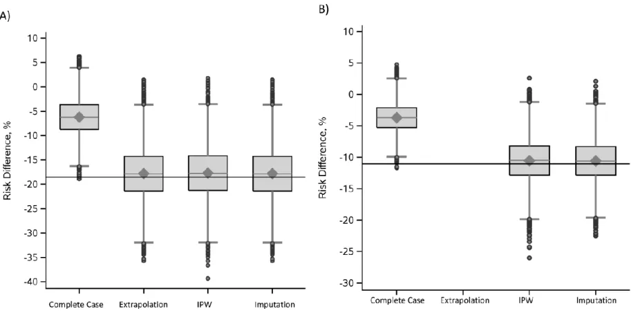
strategies in the Women's Interagency HIV Study, 1998 – 2017. ... 52 Figure 4.2. Risk of all-cause mortality under hypothetical interventions to eliminate
(Panel A) or reduce (Panel B) the prevalence of non-AIDS risk factors in the Women's
Interagency HIV Study, 1998 – 2017. ... 53 Figure 4.3. Observed versus g-computation simulated cumulative incidence of all-cause
mortality under the natural course of antiretroviral therapy initiation ... 54 Figure 5.1. Causal diagram used to generate a hypothetical cohort of 1,623 HIV-positive
women ... 69 Figure 5.2. Risk difference estimated by g-computation approach contrasting provision of
short duration versus long duration opioid prescriptions ... 70 Figure 5.3. Bias (Panel A) and standard error (Panel B) for the average treatment effect of
shortening versus lengthening opioid prescription duration ... 71 Figure 5.4. Bias (Panel A) and standard error (Panel B) for the average intervention effect
of shortening opioid prescription duration versus the status quo prescribing practice ... 72 Appendix Figure 1. Risk difference for the average treatment effect estimated by
g-computation approaches including and excluding covariate 𝑍. ... 109 Appendix Figure 2. Bias (Panel A) and standard error (Panel B) for the effect of
LIST OF ABBREVIATIONS
AIDS Acquired Immunodeficiency Syndrome ART Antiretroviral Therapy
CI Confidence Interval
IPTW Inverse Probability of Treatment Weighting IPW Inverse Probability Weighting
HCV Hepatitis C Virus
HIV Human Immunodeficiency Virus IDU Injection Drug Use
RD Risk difference
RMSE Root mean squared error RR Risk ratio
US United States
CHAPTER 1: INTRODUCTION
A. Moving Beyond Antiretroviral Therapy: Intervention Portfolios Among People with HIV Health disparities persist between people with human immunodeficiency virus (HIV) and the general population. Though acquired immunodeficiency syndrome (AIDS)-related mortality has dramatically declined in the United States (US) since the availability of highly effective combination antiretroviral therapy (ART), other causes of morbidity and mortality disproportionately affect those with HIV.1–4 Compared to the general US population, those with HIV experience a higher prevalence of comorbidities including hypertension,5 cardiovascular disease,6–9 diabetes,5,10 liver disease,11,12 and pulmonary disease.13–15 Up to 65% of people with HIV experience the co-occurrence of 2 or more chronic conditions (i.e., multimorbidity).16 In addition to this high burden of comorbidities, people with HIV experience accelerated aging with an onset of multimorbidity occurring a decade earlier than those without HIV.17–19 Consequently, the widespread adoption of ART has not closed the gap in survival for people with HIV who continue to die from non-AIDS causes 8 to 9 years earlier than those without HIV.20–22
risk of cardiovascular disease as people live longer with HIV.28–30
Cigarette smoking and alcohol are important risk factors for many chronic conditions in the general population. Both smoking and heavy alcohol use have been associated with elevated risks of hypertension,31 cardiovascular disease,31 and liver disease.32,33 Furthermore, smoking and alcohol increase inflammation, which is a known marker of early mortality.34–36 In addition to cigarette smoking being an established risk factor for pulmonary diseases,37,38 it has also been identified as a risk factor for Type 2 diabetes.39,40
While tobacco, alcohol, and inflammation are recognized as significant risk factors in the general population, their adverse effects may be more pronounced among those with HIV. Several studies have reported a higher risk of respiratory tract infections, chronic obstructive pulmonary disease, and lung cancer among smokers with HIV, suggesting a synergistic relationship between cigarette smoking and HIV infection.15,41–46 In the Veterans Aging Cohort Study, HIV status appeared to interact with alcohol consumption in increasing the risk of adverse health outcomes among men; those with HIV experienced an increased risk of physiologic injury and mortality at lower thresholds of alcohol consumption than their HIV-negative counterparts.47 With people now less likely to die of AIDS and living longer with HIV in the modern ART era, these non-AIDS risk factors are becoming important determinants of excess morbidity and mortality.
quo.46,49–51 The estimated effect of a risk factor on an outcome cannot be interpreted as the effect of intervening on that risk factor given potential unmeasured, indirect effects of the intervention on the outcome and imperfect intervention efficacy.52
While randomized controlled interventions targeting non-AIDS risk factors have demonstrated some promising results they have largely been conducted among those without HIV.
Immunocompromised health status is a common exclusion criteria in trials which has led to an existing evidence base that is more applicable to relatively healthy, non-pregnant adult populations. In a meta-analysis of smoking cessation randomized interventions, nicotine replacement therapy treatments, bupropion, varenicline, and cytisine demonstrated efficacy in quitting rates.53 However, these
interventions may have differing effects among those with HIV, or in some cases, be inadvisable. For example, in several studies varenicline has been associated with increased psychiatric symptoms among those with depression54 – a comorbidity that is extremely common among those with HIV.55 Furthermore, pharmacological based interventions may not be appropriate for women of reproductive age, particularly if pregnancy is likely. The U.S. Preventive Services Task Force has declared that there is insufficient evidence to evaluate the benefits versus harms of pharmaceutical smoking cessation aids during pregnancy.56
Most alcohol consumption interventions have also been conducted among non-generalizable study populations. Some cognitive-behavioral therapy and pharmacological-based interventions have demonstrated efficacy in short-term reductions in alcohol consumption as well as lower rates of relapse.57– 59
However, studies have been conducted primarily among those with alcohol dependence or alcohol consumption levels far beyond the national recommended safe limits.
Studies of similar interventions among people with HIV have either been absent or enrolled small, highly selective (often majority male) samples of HIV-positive individuals and evaluated only short-term effects. In behavioral smoking cessation trials,60 interventions have been highly variable and endpoints have typically been smoking cessation at 6 or 12 months, making it difficult to draw
efficacy of interventions targeting alcohol use have been conducted among high risk groups and yielded mixed results;61 no studies have evaluated the impact of lowering alcohol consumption to national recommended limits among the majority of those who consume alcohol but are not classified as heavy drinkers. Similar to the challenge of randomized controlled trials outside of HIV settings, women are often underrepresented in trials of interventions on non-AIDS-related risk factors.
Further evidence of the real-world effectiveness of existing interventions among those with HIV is necessary to guide clinical decision making. However, even in observational HIV cohorts in which collected exposure and risk factor information may enable a more accurate depiction of the experience of those with HIV in the US and improve target validity,62 women are underrepresented. Many existing studies have been restricted to men or are conducted in cohorts that include an overwhelming majority of men. The Veteran’s Aging Cohort Study is composed of 97% men which made it necessary to restrict to men while studying the interaction between HIV and alcohol consumption on physiologic injury and mortality.47 No analogous study has been conducted among women with HIV. Other large cohorts of HIV-positive individuals in the US, such as the CFAR Network of Integrated Clinical Systems, are composed of over 80% men.63 Thus, results from studies conducted in these cohorts are not necessarily generalizable to women with HIV who experience a different distribution of risk factors than men with HIV5 and may also experience differing intervention efficacy. Yet women with HIV experience far greater multimorbidity5 and have seen less improvement in life expectancy with ART than men with HIV20 which makes it imperative to study multiple interventions on non-AIDS risk factors in this group using information collected in HIV cohorts that have enrolled large samples of women.
comprehensive intervention strategies is important. It is possible that improvements in survival may require more than one intervention. For example, those who quit smoking but still engage in regular, heavy drinking may not experience a substantial delay in mortality that would otherwise be observed by intervening on both risk factors together. Synergistic relationships between interventions might also exist, with early intervention on more than one risk factor yielding a greater improvement in clinical outcomes than intervening on each risk factor separately. Comparisons of intervention combinations are critical to clinicians and policymakers in prioritizing strategies for comprehensive HIV care management.
Traditional study approaches cannot provide clinicians and policymakers with estimates of the potential improvements in outcomes among those with HIV that can be achieved by various combined interventions. Ideally, a factorial randomized trial would be conducted to evaluate sets of interventions on multiple risk factors. In light of constrained resources, the large sample size and length of follow-up period required preclude these studies from being conducted. While observational studies offer a plethora of longitudinal data on an often less selective study population, confounding is a major concern due to nonrandomized treatment. Additionally, standard approaches using multivariable regression models to address confounding fail to provide valid estimates in the presence of time-varying confounders66 and often do not give covariate marginal effects.
Recent advances in statistical software and causal inference methods offer a unique opportunity to leverage observational data to quantify the impact of potential intervention portfolios (i.e.,
combinations of interventions). Marginal structural models, most commonly estimated with inverse probability of treatment weights, can appropriately control time-varying confounding and provide
weighting in some settings.64,68 Recent illustrations of its application using available statistical software packages have now made it a viable analytic tool.46,65,68–75
B. Development and Assessment of Novel Statistical Methods: A Brief History
Causal inference methods are increasingly applied to observational data to answer pressing research questions and guide clinical decision making. For both HIV-positive populations and other vulnerable groups, there is an urgency to identify and rigorously evaluate interventions that can improve patient health outcomes. Randomized controlled trials are costly, inefficient, and infeasible in many settings. Consequently, causal inference methods play an important role in providing answers to these questions. Examples have demonstrated that under a set of “identification” assumptions, these methods can be applied to existing observational data to yield results comparable to those that would be obtained with a randomized controlled trial.66,68,75,76
The parametric g-computation estimator is one such causal inference method that is likely to become a more popular approach to assessing potential impacts of interventions. Until recently, a major barrier to the adoption of the parametric g-computation estimator was the absence of examples of its implementation using available statistical software. However, a PubMed search reveals that since Taubman et al. provided an illustration in 2009,69 there have been 75 published studies using this estimator in analyses. Given the unique flexibility of the parametric g-computation estimator and
additional guidance published in 201268 and 2014,71 it will likely become a more common analytic choice. Approaches to implement the parametric g-computation estimator in analyses assume complete exposure information; yet, missing data are extremely common in epidemiologic research.77 In previous studies using HIV observational data, this has not presented a substantial problem. This is due to the fact that in many instances to date, the research question has focused on ART based interventions.68,73,78 Because many existing observational HIV cohorts were established to study the natural and treated progression of HIV, ART information tends to be very well measured with few missing data.
Further improvements in the health outcomes and survival of people with HIV will require more
comprehensive interventions that additionally target non-AIDS risk factors; yet, sparsely collected data on non-ART exposures in existing observational data sources leaves investigators without validated
approaches to quantify such intervention effects.
In both existing HIV cohorts as well as other observational studies, exposure information may be missing by design or missing for unknown reasons. Missing data may occur by design when data
collection is expensive or was only performed on a subset of the cohort. For example, the Women’s Interagency HIV Study has additional detailed biomarker and behavioral data collected on a sample of cohort members as part of previous and ongoing substudies. (See: http://statepiaps.jhsph.edu/wihs/invest-info/dossier.pdf) Additionally, linkages to claims databases or electronic medical records can provide more detailed exposure information but may only be possible for a subset of the cohort due to cost or other barriers such as only being able to link records for people who are in regular care. To avoid loss of efficiency and potential threats to the validity of results,77,79–81 investigators need guidance regarding approaches that may be used to address missing data in the parametric g-computation framework.
findings; or 3) use ad-hoc methods to account for missing data which have not been systematically validated for g-computation.
New extensions to rigorous counterfactual-based approaches will be imperative to leverage underused observational data to evaluate and compare interventions on non-AIDS risk factors.
CHAPTER 2: STATEMENT OF SPECIFIC AIMS
A. Overview
The overall objectives of this work were to 1) leverage observational data and novel quantitative methods to estimate the impact of combined interventions to delay mortality among women with HIV and 2) refine these methods to accommodate missing exposure information that is likely to hamper crucial future studies of interventions on non-AIDS risk factors. To meet these objectives, we carried out the following specific aims using longitudinal data from HIV-positive women participating in the Women’s Interagency HIV Study (WIHS)89–91– the largest ongoing interval cohort of HIV-positive women in the United States.
B. Aim 1
We aimed to estimate the effects of alcohol consumption and smoking cessation interventions combined with prompt initiation of ART in the modern treatment era on the 8-year cumulative incidence of all-cause mortality in the WIHS between 1998 and 2017 using the parametric g-computation algorithm. Our goal was to use this approach to estimate the risks of all-cause mortality under two sets of
intervention portfolios (i.e., combined interventions) where Set A interventions were specified as the elimination of these non-AIDS risk factors and Set B interventions were specified as the reduction in the prevalence of these non-AIDS risk factors based on the expected efficacy of existing, real-world
interventions. We further aimed to estimate the impact of each intervention portfolio compared to an intervention only on prompt initiation of ART in the modern era using risk differences and ratios.
rather than reduced the prevalence of, non-AIDS risk factors would achieve the greatest improvements in survival.
Rationale: There is a high prevalence of smoking and alcohol consumption in the WIHS91–94 and other HIV-positive populations,23,24,95 both of which are known risk factors for mortality and have potentially more pronounced adverse effects among those with HIV.15,41–45,47 With ART-treated HIV-positive individuals now less likely to die from AIDS, these non-AIDS risk factors may contribute to a greater proportion of excess morbidity and mortality. Consequently, eliminating or reducing the
prevalence of smoking and alcohol consumption may improve survival in the modern ART era. Because eliminating risk factors assumes interventions with 100% efficacy and no side effects52 and existing interventions have much lower efficacy, the smaller reduction in the prevalence of smoking and alcohol consumption with real-world interventions will likely have attenuated effects on survival.
C. Aim 2
We aimed to develop, validate, and illustrate approaches to constructing two-stage g-computation estimators of the total population-level treatment and intervention effects in the presence of missing exposure information. Using a simulation study design and a hypothetical cohort simulated to represent HIV-positive women enrolled in the WIHS, our goal was to validate the following two-stage estimators. For the estimator of the average treatment effect, our goal was to construct and validate a two-stage extrapolation approach in which conditional probabilities are estimated from parametric models fit to a subset of study participants with complete exposure data; in the second stage, conditional probabilities are directly extrapolated to the full cohort. For the estimators of the average intervention effect, our goal was to construct and validate two-stage inverse probability weighted g-computation and exposure imputation g-computation approaches. We further aimed to compare the performance of each of the proposed estimators in terms of bias, standard error, 95% confidence limit coverage, and root mean squared error.
estimator will provide unbiased estimates of the absolute and relative risks for an “always treated” and “never treated” population, provided all covariates predicting both missingness and the outcome are included in models. Similarly, the two-stage inverse probability weighted and exposure imputation g-computation estimators will provide unbiased estimates of risks for an “always treated” population compared to the population under the “natural treatment course” (i.e., no imposed intervention).
Rationale: When exposure information is missing not at random, absolute and relative risks estimated from those with complete information will not necessarily equal those that would have been observed among the full cohort of interest. Two-stage g-computation approaches that leverage available covariate and outcome information from all individuals, including those with missing exposure
CHAPTER 3: METHODS
A. Overview
This chapter presents the study design, data source, assessment of measures, and statistical methods as they relate to Aims 1 and 2. The chapter is organized as follows. Section A presents a brief overview of the parametric g-computation algorithm – the approach that is used in Aim 1 analyses to estimate the effects of interventions on non-AIDS risk factors and extended in Aim 2 to accommodate missing exposure information when estimating treatment and intervention effects. In Section B, we outline the study sample, variable measurement, and analyses for Aim 1. In Section C, we outline the study design, developed estimators, and analyses for Aim 2.
A1. Parametric G-computation Estimator of the Parametric Generalized-Formula
In this document, we make the following distinction between the terminology “g-formula” and the “parametric g-computation estimator.” We use “g-formula” to refer to an equation that is used to express the observed data distribution as the distribution of the data that would have been observed under an alternative treatment plan. We use “parametric g-computation estimator” to refer to a parametric estimator of the g-formula equation. We also use “algorithm” interchangeably with “estimator.”
The parametric g-computation formula estimator67 is a recently illustrated approach68,69,71,78,97–99 to estimating the parameters of a marginal structural model. Analogous to an inverse probability of
treatment weighted (IPTW) estimator of the parameters of a marginal structural model,66,76,100 the g-computation estimator is a generalization of standardization. In longitudinal observational study settings subject to time-varying confounding, both IPTW and g-computation estimators can provide valid
Three particular advantages of the parametric g-computation estimator are its flexibility in estimating population-level effects of realistic changes to exposure distributions,46,49,51,65,74,102,103 ability to estimate effects of interventions that depend on the natural value of exposure,104,105 and efficiency in quantifying impacts of multiple interventions.69,105 Whereas the IPTW estimator has been widely used to obtain contrasts of an “always treated” versus “never treated” population, this is often not representative of the scenarios that policymakers are considering.49,51 For example, in deciding whether more resources should be allocated to smoking cessation interventions, the alternative to targeting more smokers for treatment is not “take away treatment from all smokers”; rather, it is more likely that the alternative is “maintain the status quo.” The parametric g-computation estimator can easily be specified to provide such contrasts. The extended parametric g-computation estimator can also be used to specify interventions that involve changes to exposure that depend on the natural value of exposure that would be observed if intervention were discontinued immediately before measurement.104,105 An example of an intervention that depends on the natural value of exposure is “intervene to eliminate depression with probability 66% if depression occurs without intervening immediately before this timepoint.”64 Finally, while the IPTW estimator can become inefficient when estimating multiple joint interventions, the g-computation estimator relies on more parametric models, and consequently, may maintain a higher level of efficiency.64,106
A2. Identification Conditions
Under a sufficient set of conditions, the g-computation formula re-expresses the distribution of the data under the observed treatment (i.e., the factual) as the distribution of the data that would have been observed under a potentially alternative treatment (i.e., the counterfactual). Mathematically, this can be written in a simplified, time-fixed setting as shown below where the left-hand side of the equation
∑ 𝐸(𝑌 = 𝑦|𝐴 = 𝑎, 𝑊 = 𝑤)𝑃(𝑊 = 𝑤) = 𝐸{𝑌(𝑎) = 𝑦}
𝑤
The identification conditions are as follows:
1) No measurement error of treatment, covariates, or outcome.107 More specifically, we assume that the treatment and outcome are measured without error while covariates might be mismeasured but that the observed covariate values are those that inform the treatment plan. For example, a laboratory measurement of CD4 cell count might be 220 for a patient whose true CD4 cell count is 235; however, the 220 value the clinician sees is the value that is used to determine whether or not to initiate ART.
2) Counterfactual consistency (also described as treatment version irrelevance and no
interference).108,109 If the observed treatment of patient i is equal to the treatment of interest (i.e., 𝐴𝑖 = 𝑎), then the observed outcome of patient i is equal to the outcome that would have been observed if treatment was set to the treatment of interest (i.e., 𝑌𝑖 = 𝑌𝑖(𝑎)).
3) Conditional exchangeability or no unmeasured confounding.110 The probability of treatment conditional on a set of covariates is independent of the potential outcome (i.e.,
𝑃(𝐴 = 𝑎|𝑊 = 𝑤, 𝑌(𝑎)) = 𝑃(𝐴 = 𝑎|𝑊 = 𝑤)).
4) Positivity, also described as the experimental treatment assignment assumption.111 The conditional probability of receiving treatment is nonzero within all strata of covariates (i.e.,
𝑃(𝐴 = 𝑎|𝑊 = 𝑤) > 0).
5) Correct specification of parametric models.
B. Aim 1: Interventions on Non-AIDS Risk Factors among Women with HIV
B1. Data Source and Study Population
The Women’s Interagency HIV Study (WIHS) is an ongoing, multisite prospective cohort study of HIV-positive and HIV-negative women in the US.89–91 Though the WIHS was initially established in 1993 to study the progression of HIV infection in women,89 its research focus has since expanded to other areas including aging, behavioral and social health determinants, comorbidities, and epidemiologic methods.91 As shown in Figure 3.1, the WIHS includes 10 consortia of contributing sites, 6 of which began in 1994 (Bronx/Manhattan, NY; Brooklyn, NY; Chicago, IL; Los Angeles/Southern CA/Hawaii; San Francisco/Bay Area, CA; Washington, DC) and 4 of which were added in 2013 (Atlanta, GA; Birmingham, AL/Jackson, MS; Chapel Hill, NC; Miami, FL). The Baltimore, MD site has served as the data coordinating center since 1997.
Figure 3.1. Women’s Interagency HIV Study and data coordinating center sites.
Source: https://wihs.gumc.georgetown.edu/aboutwihs/partnersites
and longest ongoing prospective cohort study of women with HIV in the US. In other large clinical cohorts of people with HIV in the US, women (especially non-White women) are a small minority, limiting generalizability among this population. Thus, the WIHS is one of the leading cohorts for studies among women with HIV in the US.
WIHS participants attend study visits every 6 months, during which they contribute extensive demographic, medical history, medication use, health service utilization, and behavioral data through in person interviews. During visits, participants also undergo clinical examination including vital sign measurements, anthropometric measurements, and a gynecological exam. Blood, urine, and
cervicovaginal swab samples are collected. Data from study visits are supplemented with medical record abstractions and linkages to cancer and death registries.
B2. Study Inclusion and Exclusion Criteria
Since 1994, the WIHS has enrolled 4982 women, 3703 of whom were HIV-positive at baseline or seroconverted over follow-up. Eligibility for Aim 1 of the proposed study was restricted to HIV-positive women with a study visit on, or after, 1 April 1998 and who had not previously initiated ART (N=1033). The analysis baseline for each woman was defined as the woman’s first HIV-positive WIHS study visit on, or after, 1 April 1998. For women enrolled in Wave 1 (1994-1995), the analysis baseline date occurred after the date at which they entered the WIHS. For women enrolled in all other waves, the analysis baseline date was equal to the WIHS entry date if they were HIV-seropositive at entry; otherwise, it occurred after their WIHS entry date if they seroconverted over follow-up.
We defined the baseline visit as occurring on, or after, 1 April 1998 because our research
questions were relevant to the calendar period in which highly effective, triple therapy combination ART was widely available. It was after the introduction of these regimens in 1997112 that AIDS-related
visits occur on 1 April and 1 October each year – hence, the inclusion of visits occurring at/after 1 April 1998. All follow-up visits after each woman’s analysis baseline date were included.
Women who had already initiated 3-drug combination ART prior to the analysis baseline date were not included. This was to accommodate a new-user design in regards to ART treatment.113 In observational study settings, new-user designs are recommended to eliminate biases that arise when prevalent users are included in analyses. Namely, new-user designs prevent survivor bias in regards to prevalent users that survive early periods of pharmacotherapy and bias resulting from confounders that are affected (i.e., mediated) by the treatment.
Among 1033 HIV-positive combination ART-naïve women with a study visit on/after 1 April 1998, we excluded 2% of the sample for missing information on key baseline variables. We excluded women with missing baseline information on depression (n=17), alcohol consumption (n=9), and smoking status (n=8). In the remaining sample of 1016 HIV-positive women, we imputed 5 (0.5%) missing baseline CD4 counts and 18 (1.8%) missing baseline viral load counts by simulation from log normal distributions with mean and standard deviation equal to that of the observed WIHS sample at baseline. The final sample for analysis included N=1016 HIV-positive, combination ART-naïve, women. B3. Exposures and Outcome
Information on ART, alcohol consumption, and smoking exposures have been collected on WIHS participants via in-depth interviews at all baseline and follow-up visits. Combination ART is determined using a definition based on Department of Health and Human Services/Kaiser Panel guidelines.114 Women are considered to be on combination ART if they report use of 3+ antiretroviral drugs, one of which is a protease inhibitor (PI), a non-nucleoside reverse transcriptase inhibitor (NNRTI), an integrase inhibitor (II), or an entry inhibitor (EI). During interviews, women also reported the number of drinks consumed on average per week and smoking status since the last visit.
data are available from 2000 until present. In both state and national death registries, data include the date and location of death as well as the International Classification Diseases (ICD) codes for the underlying and contributing causes of death. Our outcome of interest was all-cause mortality and was defined as a documented death from any cause.
B4. Interventions
Our primary objective was to estimate the risk115,116 of all cause-mortality in the WIHS under hypothetical intervention portfolios (i.e., intervention combinations) targeting prompt initiation of modern ART, alcohol, and smoking. In our base scenario (Portfolio 1), we considered an intervention solely on prompt initiation of modern ART to represent the “status quo” in regards to the current recommended healthcare guidelines among people with HIV. We defined modern ART as combination ART initiated on/after 1 October 2001. This date coincides with the period after which tenofovir had been approved and became a common drug in combination ART regimens.114 “Prompt” initiation was defined as initiation of ART by 6 months of baseline (i.e., being on ART at the first follow-up visit). This definition was
influenced by the structure of the WIHS as an interval cohort with exposure status documented at the time of each 6-month follow-up visit. Because ART initiation dates are documented as the first WIHS study visit date at which an individual reported being on ART, it was not possible to decipher the exact point at which the individual initiated ART in the period between the last ART-naïve study visit and the next follow-up.
Set A intervention portfolios were defined as follows. Portfolio 2A was an intervention to eliminate alcohol consumption of over 1 drink per week among women without an indication of hepatitis C virus (HCV) and eliminate all alcohol consumption among women with an indication of HCV. HCV status was determined based on bloodwork performed on all WIHS participants at baseline. If women were positive for HCV antibody, they received testing for HCV RNA to determine whether the infection was active. Here, we defined an indication of HCV to be a positive antibody test and a positive or missing HCV RNA test. We chose a limit of 1 drink per week instead of complete abstinence among those
without HCV due to potential protective effects of alcohol at low levels117 but did not define the intervention to increase drinking among those who were already abstainers. Because alcohol is
particularly harmful for those with hepatitis C infection,118 the intervention dictated complete abstinence from alcohol for these women. Portfolio 3A was defined as an intervention to eliminate smoking among all smokers. Finally, Portfolio 4A was an intervention that imposed both alcohol elimination and smoking cessation strategies.
Set B intervention portfolios combining prompt initiation of modern ART with realistic reductions in the prevalence of alcohol consumption and/or smoking were defined as follows. Portfolio 2B combined prompt initiation of modern ART with an intervention to reduce alcohol consumption of over 3 drinks per week to a 3 drink per week limit among those without an indication of HCV. While current guidelines classify alcohol consumption of over 7 drinks per week for women as “heavy drinking” beyond safe limits,119 they refer to the general population and are not specific to those with HIV. Thus, to account for recent evidence suggesting that those with HIV are adversely impacted by alcohol at lower thresholds of consumption than the general population,47 we considered women consuming over 3 drinks per week for this intervention.
regarding the interaction between alcohol and HCV on liver fibrosis and effects of alcohol on antiviral treatment, and advice regarding changes to consumption. Patients had a follow-up visit 4 to 8 weeks later with a psychiatric clinical nurse specialist at which they were provided cognitive-behavioral therapy techniques and motivational enhancement therapy for coping with cravings and preventing relapse. Among those who received the intervention, 36% achieved abstinence and 26% achieved >50% reduction in drinking levels after 8 months of follow-up.120 Thus, we defined our intervention among those with an indication of HCV at baseline as a 0.36 probability of quitting alcohol, 0.26 probability of reducing consumption by 50%, and 0.38 probability of no change in alcohol consumption levels.
Portfolio 3B was defined as a behavioral smoking cessation intervention described by Hoffman et al121 and tested in the WIHS. The intervention consisted of stage-based Transtheoretical model (TTM) tailored health communications on smoking cessation delivered via computer expert systems in waiting rooms at primary care clinics. The intervention was delivered at baseline, 3 months, and 6 months. Participants also received audiotapes relevant to their stage of change. At six months, 16.3% of
participants had quit smoking. Thus, we defined our intervention among smokers as a 0.16 probability of quitting smoking.
The combination of the alcohol and smoking cessation interventions described above was defined as Portfolio 4B.
B5. Covariates of Interest
confounders is shown in the figure though various elements from this set functioned as subsets of confounding variables for each exposure. Time-varying covariates included CD4 count, viral load, and depression.
We also considered a time-updated measure of visit number, interactions between time and each of the exposures (i.e., ART, alcohol, smoking) and interactions between exposures.
Figure 3.2. Causal Diagram of ART, Non-AIDS Risk Factors, and Mortality.*
B6. Treatment Decision Design
The overall analytic goal of Aim 1 was to use rich, longitudinal data collected from the WIHS to obtain estimates of the potential reductions in the cumulative incidence of mortality that could be achieved by multiple interventions on non-AIDS risk factors. A defined set of criteria was used to determine eligibility for intervention among each WIHS participant at each study visit, with analyses structured in the format of a treatment decision design.123 The treatment decision design is a
generalization of the new-user design113 which anchors a cohort’s follow-up to times at which treatment decisions are made. While all WIHS participants meeting the inclusion criteria defined in Section B2 were eligible for inclusion in the analysis sample, only WIHS participants with a specific risk factor at a given visit were considered eligible for the intervention at that visit. We used semi-annual study visits to represent the timepoints at which intervention decisions were made. At each visit, women’s risk factor information was used to determine eligibility for each intervention as described below.
ART: Because all women in the analysis sample were ART-naïve at baseline, they were all considered eligible for the intervention on prompt initiation of ART in the modern treatment era. Thus, all women were eligible to initiate ART by the first follow-up visit. Once women initiated ART, they were assumed to remain on ART and were no longer considered for ART initiation at later semi-annual visits.
Alcohol reduction: Both HCV status and alcohol consumption levels determined eligibility for the alcohol reduction intervention. Specifically, women with an indication of HCV at baseline were eligible for the alcohol intervention if they reported consumption of any alcohol at a given visit. Women without an indication of HCV at baseline were considered for the alcohol elimination intervention (Portfolio 2A) if they reported consumption of over 1 drink per week and for the alcohol reduction intervention
(Portfolio 2B) if they reported consumption of over 3 drinks per week at a given visit. Women could receive this intervention multiple times.
B7. Notation and Parameters of Interest
Let uppercase letters denote random variables and lowercase letters denote potential realizations of those variables. Let 𝑖 index 1, …, 1016 women in our study sample, 𝑗 index 1, …, 𝐽 completed visits of follow-up, and 𝑌𝑖𝑗 represent an indicator of death for woman 𝑖 at time 𝑗. The maximum number of follow-up visits is 𝐽 = 16; as WIHS visits occur every 6 months, this corresponds to 8 years of follow-up since study baseline. We use 𝐴𝑖𝑗 to represent a binary indicator of antiretroviral therapy (ART) treatment,
𝐷𝑖𝑗 to represent categorical indicators for average drinking level per week since the last study visit and 𝑆𝑖𝑗 to represent a binary indicator of smoking. We use 𝒁𝑖𝑗to represent a vector of time-varying covariates for woman 𝑖 measured at time 𝑗 (i.e., CD4 count, detectable viral load, and depression) and 𝑾𝑖𝑗 to represent a vector of time-fixed demographic and clinical characteristics for woman 𝑖 measured at baseline (i.e., 𝑗 = 0). The vector 𝑾𝑖𝑗 includes baseline age, race, level of education, history of injection drug use (IDU), prior exposure to dual therapy zidovudine (AZT), wave of WIHS enrollment, CD4 count, viral load, and smoking status. Finally, we use 𝐶𝑖𝑗 to represent a binary indicator of being censored due to being lost to follow-up which we defined as having two consecutive missed WIHS visits. All women were
administratively censored after a maximum of 8 years of completed follow-up due to sparse data at later time points. To accommodate sporadic missing data for time-varying covariates and exposures in the observed data, we used a last observation carried forward approach.
At each timepoint 𝑗, the temporal ordering of variables is: 𝑾𝑖𝑗; 𝐶𝑖𝑗;𝑌𝑖𝑗; 𝐴𝑖𝑗, 𝐷𝑖𝑗, 𝑆𝑖𝑗; 𝒁𝑖𝑗. The values of the time-fixed covariates 𝑾𝑖𝑗 remain constant for each woman throughout the study period so that for a given woman 𝑖,𝒘𝑖0 = 𝒘𝑖1=. . . = 𝒘𝑖𝐽. Among those who remained uncensored and alive by visit 𝑗 (i.e., 𝐶𝑖𝑗 = 𝑌𝑖𝑗 = 0), values of ART (i.e., 𝐴𝑖𝑗), drinking level (i.e., 𝐷𝑖𝑗), and smoking (i.e., 𝑆𝑖𝑗) were measured based on self-report corresponding to the 6-month period between 𝑗 − 1 and 𝑗.
It should be noted that while exposures to ART, drinking level, and smoking occurred between
a change in exposure status in the time period between the last follow-up visit at which they remained alive (and uncensored) and their death date. ART initiation dates are recorded as the first WIHS visit date at which individuals report having initiated ART, while death dates are recorded as actual dates of death. Therefore, we assume that those who had not initiated ART at the last visit at which they remained alive and uncensored did not do so before a death occurring before the next scheduled follow-up visit.
Similarly, we assume drinking and smoking status did not change between the last visit at which women remained alive and uncensored and their death. Or rather, in both cases, we assume that any change in ART, drinking, or smoking between the last follow-up visit and a death occurring less than 6 months later was too short of an exposure period to notably affect the risk of death.
Among those who remain alive and uncensored at time 𝑗, measured values of time-varying covariates (i.e., 𝒁𝑖𝑗) correspond to real time, or nearly real time, measures at 𝑗. Specifically, CD4 cell count and viral load were measured by laboratory tests conducted at the time of the WIHS visit. Depression was measured by a validated questionnaire124 that asked women to report symptoms experienced during the last week. In the remaining text we suppress subscript 𝑖.
The cumulative incidence of mortality in the WIHS under the observed exposure history (i.e., no intervention on ART initiation or non-AIDS risk factors) at time 𝑗 can be expressed as Equation 1:
𝐹(𝑗) = ∑ ∑ ∑ ∑ ∑ ∑
{
𝑃(𝑌𝑘+1= 1|𝐴̅𝑘= 𝑎̅𝑘, 𝐷̅𝑘= 𝑑̅𝑘, 𝑆̅𝑘= 𝑠̅𝑘, 𝒁̅𝑘= 𝒛̅𝑘, 𝑾𝑘= 𝒘𝑘, 𝐶̅𝑘= 𝑌̅𝑘= 0) ×
∏
[
𝑓(𝒁𝑚|𝐴̅𝑚−1= 𝑎̅𝑚−1, 𝐷̅𝑚−1= 𝑑̅𝑚−1, 𝑆̅𝑚−1= 𝑠̅𝑚−1, 𝒁̅𝑚−1= 𝒛̅𝑚−1, 𝑾𝑚= 𝒘𝑚, 𝐶̅𝑚= 𝑌̅𝑚= 0) ×
𝑃(𝑆𝑚= 𝑠𝑚|𝐷̅𝑚−1= 𝑑̅𝑚−1, 𝑆̅𝑚−1= 𝑠̅𝑚−1, 𝒁̅𝑚−1= 𝒛̅𝑚−1, 𝑾𝑚= 𝒘𝑚, 𝐶̅𝑚= 𝑌̅𝑚= 0) ×
𝑃(𝐷𝑚= 𝑑𝑚|𝐷̅𝑚−1= 𝑑̅𝑚−1, 𝒁̅𝑚−1= 𝒛̅𝑚−1, 𝑾𝑚= 𝒘𝑚, 𝐶̅𝑚= 𝑌̅𝑚= 0) ×
𝑃(𝐴𝑚= 𝑎𝑚|𝐴̅𝑚−1= 𝑎̅𝑚−1, 𝐷̅𝑚−1= 𝑑̅𝑚−1, 𝑆̅𝑚−1= 𝑠̅𝑚−1, 𝒁̅𝑚−1= 𝒛̅𝑚−1, 𝑾𝑚= 𝒘𝑚, 𝐶̅𝑚= 𝑌̅𝑚= 0) ×
𝑃(𝑌𝑚= 0|𝐴̅𝑚−1= 𝑎̅𝑚−1, 𝐷̅𝑚−1= 𝑑̅𝑚−1, 𝑆̅𝑚−1= 𝑠̅𝑚−1, 𝒁̅𝑚−1= 𝒛̅𝑚−1, 𝑾𝑚= 𝒘𝑚, 𝐶̅𝑚−1= 𝑌̅𝑚−1= 0) ×
𝑓(𝑾𝑚) × ]
𝑘 𝑚=0 } 𝑗 𝑘=0 𝒘𝑗 𝑎̅𝑗 𝑑̅𝑗 𝑠̅𝑗 𝒛̅𝑗
follow-up visit could not have initiated modern ART. This is based on our definition of modern ART initiation as initiation of ART on, or after, 1 October 2001 (the period after which tenofovir had been approved and became a common drug in combination ART regimens).114 However, we used observed exposure information from those in the modern treatment era to extrapolate modern ART to this earlier time period. The adapted equation is written as Equation 2:
𝐹𝑎𝑔
(𝑗) = ∑ ∑ ∑ ∑ ∑
{
𝑃(𝑌𝑘+1= 1|𝐴̅𝑘−1 𝑔
= 𝑎̅𝑘𝑔, 𝐷̅𝑘= 𝑑̅𝑘, 𝑆̅𝑘= 𝑠̅𝑘, 𝑾𝑘= 𝒘𝑘, 𝐶̅𝑘= 𝑌̅𝑘= 0) ×
∏
[
𝑓(𝒁𝑚|𝐴̅𝑚−1 𝑔
= 𝑎̅𝑚−1 𝑔
, 𝐷̅𝑚−1= 𝑑̅𝑚−1, 𝑆̅𝑚−1= 𝑠̅𝑚−1, 𝒁̅𝑚−1= 𝒛̅𝑚−1, 𝑾𝑚= 𝒘𝑚, 𝐶̅𝑚= 𝑌̅𝑚= 0) ×
𝑃(𝑆𝑚= 𝑠𝑚|𝐷̅𝑚−1= 𝑑̅𝑚−1, 𝑆̅𝑚−1= 𝑠̅𝑚−1, 𝒁̅𝑚−1= 𝒛̅𝑚−1, 𝑾𝑚= 𝒘𝑚, 𝐶̅𝑚= 𝑌̅𝑚= 0) ×
𝑃(𝐷𝑚= 𝑑𝑚|𝐷̅𝑚−1= 𝑑̅𝑚−1, 𝒁̅𝑚−1= 𝒛̅𝑚−1, 𝑾𝑚= 𝒘𝑚, 𝐶̅𝑚= 𝑌̅𝑚= 0) ×
1 × 𝑃(𝑌𝑚= 0|𝐴̅𝑚−1
𝑔
= 𝑎̅𝑚−1 𝑔
, 𝐷̅𝑚−1= 𝑑̅𝑚−1, 𝑆̅𝑚−1= 𝑠̅𝑚−1, 𝒁̅𝑚−1= 𝒛̅𝑚−1, 𝑾𝑚= 𝒘𝑚, 𝐶̅𝑚−1= 𝑌̅𝑚−1= 0) ×
𝑓(𝑾𝑚) ]
𝑘 𝑚=0 } 𝑗 𝑘=0 𝒘𝑗 𝑑̅𝑗 𝑠̅𝑗 𝒛̅𝑗
where we use superscript 𝑔 to convey that the value of 𝐴 is being set according to the intervention plan. Equation 2 can be further adapted to express the cumulative incidence of mortality in the WIHS under universal, prompt initiation of ART in the modern treatment era combined with various
interventions on alcohol consumption and/or smoking. Because these interventions depend on the natural value of alcohol consumption and smoking, this requires use of the extended version of the parametric g-computation estimator.104,105 This facilitates the expression of interventions that are implemented based on the values of alcohol and smoking that would be observed if intervention were discontinued immediately before measurement at time 𝑗. The incidence function under these additional interventions can be
expressed with the extended parametric g-formula as Equation 3: 𝐹(𝑎,𝑑,𝑠)𝑔
(𝑗)
= ∑ ∑ ∑ ∑ ∑
{
𝑃(𝑌𝑘+1= 1|𝐴̅𝑘 𝑔
= 𝑎̅𝑘 𝑔
, 𝐷̅𝑘𝑔
= 𝑑̅𝑘 𝑔
, 𝑆̅𝑘𝑔
= 𝑠̅𝑘 𝑔
, 𝒁̅𝑘= 𝒛̅𝑘, 𝑾𝑘= 𝒘𝑘, 𝐶̅𝑘= 𝑌̅𝑘= 0) ×
∏
[
𝑓(𝒁𝑚|𝐴̅𝑚−1 𝑔
= 𝑎̅𝑚−1 𝑔
, 𝐷̅𝑚−1𝑔
= 𝑑̅𝑚−1 𝑔
, 𝑆̅𝑚−1 𝑔
= 𝑠̅𝑚−1 𝑔
, 𝒁̅𝑚−1= 𝒛̅𝑚−1, 𝑾𝑚−1= 𝒘𝑚−1, 𝐶̅𝑚= 𝑌̅𝑚= 0) ×
𝑃𝑔(𝑆 𝑚
𝑔
= 𝑠𝑚 𝑔
|𝑆𝑚∗ = 𝑠𝑚∗, 𝐷̅𝑚−1 𝑔
= 𝑑̅𝑚−1 𝑔
, 𝑆̅𝑚𝑔
= 𝑠̅𝑚 𝑔
, 𝒁̅𝑚−1= 𝒛̅𝑚−1, 𝑾𝑚−1= 𝒘𝑚−1, 𝐶̅𝑚= 𝑌̅𝑚= 0) ×
𝑃𝑜𝑏𝑠(𝑆
𝑚∗ = 𝑠𝑚∗|𝐷̅𝑚−1 𝑔
= 𝑑̅𝑚−1 𝑔
, 𝑆̅𝑚−1 𝑔
= 𝑠̅𝑚−1 𝑔
, 𝒁̅𝑚−1= 𝒛̅𝑚−1, 𝑾𝑚−1= 𝒘𝑚−1, 𝐶̅𝑚= 𝑌̅𝑚= 0) ×
𝑃𝑔(𝐷 𝑚 𝑔
= 𝑑𝑚 𝑔
|𝐷𝑚∗ = 𝑑𝑚∗, 𝐷̅𝑚−1 𝑔
= 𝑑̅𝑚−1 𝑔
, 𝒁̅𝑚−1= 𝒛̅𝑚−1, 𝑾𝑚−1= 𝒘𝑚−1, 𝐶̅𝑚= 𝑌̅𝑚= 0) ×
𝑃𝑜𝑏𝑠(𝐷
𝑚∗ = 𝑑𝑚∗|𝐷̅𝑚−1 𝑔
= 𝑑̅𝑚−1 𝑔
, 𝒁̅𝑚−1= 𝒛̅𝑚−1, 𝑾𝑚−1= 𝒘𝑚−1, 𝐶̅𝑚= 𝑌̅𝑚= 0) ×
1 × 𝑃(𝑌𝑚= 0|𝐴̅𝑚−1
𝑔
= 𝑎̅𝑚−1 𝑔
, 𝐷̅𝑚−1 𝑔
= 𝑑̅𝑚−1 𝑔
, 𝑆̅𝑚−1 𝑔
= 𝑠̅𝑚−1 𝑔
, 𝒁̅𝑚−1= 𝒛̅𝑚−1, 𝑾𝑚−1= 𝒘𝑚−1, 𝐶̅𝑚−1= 𝑌̅𝑚−1= 0) ×
𝑓(𝑾𝑚) ]
𝑘 𝑚=0 } 𝑗 𝑘=0 𝒘𝑗 𝑑̅𝑗 𝑠̅𝑗 𝒛̅𝑗
these variables. The value 𝑎̅𝑗𝑔 is set to 1 across all 𝑗 ≥ 1 for each set of intervention portfolios while the values of 𝑑̅𝑗𝑔 and 𝑠̅𝑗𝑔 are set according to the plans described in Section B4.
B8. Implementation of Parametric G-computation
We used the parametric g-computation estimator67–69,71,72,78,99,105 to estimate the equations in Section B7. Namely, we estimated the 8-year cumulative incidence of all-cause mortality under the natural course, the 8-year cumulative incidence of all-cause mortality under prompt initiation of modern ART, and the 8-year cumulative incidences of all-cause mortality under each set of intervention
portfolios. Furthermore, we estimated the 8-year risk differences and ratios contrasting each intervention portfolio to an intervention solely on prompt initiation of modern ART. The steps to using the
g-computation estimator to parametrically estimate the g-g-computation formula have been previously described.68,69,71 Briefly, we implemented g-computation in our setting as follows.
Steps 1 – 3: First, we fit pooled person-visit logistic and linear models to the observed data
across all visits 𝑗 ≥ 1 to estimate the conditional probability or density of each exposure, time-varying covariate, and outcome. Specifically, we fit models for ART initiation, alcohol consumption, smoking, CD4 cell count, viral load, depression, and death. Second, we estimated conditional probabilities or densities from these models. Third, we drew a large Monte Carlo sample of 𝑁 = 100,000 women at baseline (i.e., 𝑗 = 0) with replacement.
outcome distribution under the natural course (Equation 1 in Section B7). By natural course, we mean no intervention (i.e., no manipulation of treatment status).
To achieve this, we first fit intercept only models to the pooled person-visit data for each time-varying covariate, exposure, and outcome with indicator variables for visit number as the only predictor. We then compared the distribution of each variable at each visit in the Monte Carlo dataset with the distribution of each variable at each visit in the original WIHS dataset. Further complexity was then incorporated into each of the models by adding relevant covariates (e.g., hypothesized confounders, predictors of the dependent variable) and interactions and adapting functional forms. After each specification of the set of models, conditional probabilities or densities were estimated and saved from each model, a Monte Carlo sample of size 100,000 was drawn from the baseline data with replacement, follow-up data were generated at each follow-up visit from the saved conditional probabilities or
densities, and the distribution of variables in the Monte Carlo dataset were compared with the distribution in the WIHS dataset using figures and summary statistics (e.g., frequencies, mean/median/standard deviation). We also assessed interaction terms using Likelihood Ratio Tests for interaction.
We estimated the cumulative incidence of mortality at each time point using the complement of the Kaplan-Meier125 (product-limit) estimator of the survival function. The estimator can be expressed as:
𝑆̂(𝑗) = ∏ (1 −𝑑𝑘 𝑛𝑘
)
𝑗
𝑘=1
where 𝑑𝑘 denotes the number of deaths at discrete time 𝑘, 𝑛𝑘 denotes the number at risk at discrete time
𝑘, and 𝑆̂(𝑗) denotes the estimated survival at time 𝑗.
in the observed WIHS data. Discrepancies can arise from improper model specification as well as finite sample bias resulting from sparse data.
Thus, to improve model fit, we repeated the above Steps 1 – 4 using flexible specifications of continuous and categorical variables, interaction terms, and various sets of covariates for each model until we 1) had included all hypothesized confounders relevant to each exposure, and 2) were able to replicate distributions observed in the WIHS sample in the Monte Carlo sample. The variables and models that were selected for final analyses are described in Appendix A of the Supplemental Text.
Step 5: Once we were able to replicate the empirical distribution of covariates and outcome in the Monte Carlo sample, we used the finalized models to simulate outcomes under the interventions of interest. We repeated Steps 1 – 4, altering exposure values according to the defined interventions and simulated follow-up data using the saved conditional probabilities or densities.
Step 6: We estimated the cumulative risk of all-cause mortality at each follow-up visit in each dataset using the complement of the Kaplan-Meier125 (product-limit) estimator of the survival function. We censored all women at a maximum of 16 follow-up visits (i.e., 8 years of follow-up) due to sparse data at later time points. We output the cumulative risks at each timepoint and concatenated datasets. To quantify the impact of scaling up interventions on non-AIDS risk factors, we contrasted the estimated risk of all-cause mortality under each intervention portfolio with the estimated risk under intervening on prompt initiation of ART in the modern treatment era alone using risk differences and risk ratios.
Step 7: We repeated the above steps on 1000 nonparametric bootstrap126 samples to obtain standard errors calculated as the standard deviation of point estimates across bootstraps. We used standard errors to calculate 95% confidence intervals.
C1. Motivating Example
The primary example for our development and assessment of two-stage g-computation estimators focused on a simplified time-fixed scenario. In the first part of the scenario, interest was in obtaining unbiased estimates of the covariate vector 𝑾 standardized risk of an outcome 𝑌 in an HIV cohort under scenarios in which the entire cohort did not receive versus did receive a harmful treatment 𝐴. This parameter is known as the average treatment effect.46,49,88,103 In the second part of the scenario, interest was in obtaining unbiased estimates of the covariate vector 𝑾 standardized risk of an outcome 𝑌 in the HIV cohort under a scenario in which an intervention removed treatment 𝐴 versus treatment practices remained the same (i.e., the natural course or status quo). This parameter is known as the average
intervention effect.46,49,51,88,103 More specifically, it represents a special case of an generalized intervention effect in which the intervention is 100% efficacious.51
While it is straightforward to implement the parametric g-computation estimator to obtain estimates of these parameters when data are complete, this is no longer the case when faced with partially missing exposure information. If estimates are desired for the total study population but treatment status is only observed on a subset (i.e., where 𝑅 = 1) complications arise, especially if there are other variables associated with the outcome that additionally influence whether or not treatment status is observed; in other words, if there exists a variable 𝑍 associated with both 𝑅 and 𝑌.