BAYESIAN INFLUENCE DIAGNOSTIC
METHODS FOR PARAMETRIC REGRESSION
MODELS
Hyunsoon Cho
A dissertation submitted to the faculty of the University of North Carolina at Chapel Hill in partial fulfillment of the requirements for the degree of Doctor of Philosophy in the Department of Biostatistics, Gillings School of Global Public Health.
Chapel Hill 2009
Approved by:
Dr. Joseph G. Ibrahim, Advisor Dr. Hongtu Zhu, Co-advisor Dr. Gary G. Koch, Reader Dr. Haitao Chu, Reader
c
° 2009
ABSTRACT
HYUNSOON CHO: BAYESIAN INFLUENCE DIAGNOSTIC METHODS FOR PARAMETRIC REGRESSION MODELS. (Under the direction of Dr. Joseph G. Ibrahim and Dr. Hongtu Zhu.)
The goals of assessing the influence of individual observations in statistical analy-sis are not only to identify influential observations such as outliers and high leverage points, but also to determine the importance of each observation in the analysis for a better model fit. Thus, assessing the influence of individual observations on a model, choosing an appropriate dimensionality of a model and selecting the best model for a given dataset are very important and highly relevant problems in any formal statistical analysis.
Recently, Bayesian methodologies have been getting enormous attention in biomed-ical research due to the potential advantages of fitting a vast array of complex models posed by modern data. As the demand for Bayesian data analysis and modeling in-creases, we need good diagnostic methods for model assessment and selection. In this dissertation, we develop Bayesian diagnostic measures based on case-deletion to assess the influence of each observation to model fit and model complexity. First, we propose Bayesian case influence diagnostics for complex survival models. In detail, we develop case deletion influence diagnostics for both the joint and marginal posterior distri-butions based on the Kullback-Leibler divergence. Second, we introduce three types of Bayesian case influence measures based on case deletion, namely the φ-divergence,
their applications to identification of influential sets and model complexity.
ACKNOWLEDGMENTS
I have been very fortunate to have great mentors and friends during my journey of graduate studies. I would especially like to thank my advisor, Dr. Joseph Ibrahim, for his mentorship, advice and financial support during the completion of this dissertation. His genuine advice and leadership as a mentor guided me to a successful completion of my graduate studies. Also, I would like to thank Dr. Hongtu Zhu, who also served as my advisor, for his important contributions and guidance. He helped me to get through the difficult problems. I would like to express my deepest appreciation to Dr. Gary Koch for his generosity with time, advice and financial support. His advice and help for my consulting work at Biometric Consulting Laboratory (BCL) as well as for my life as a biostatistician were priceless. In addition, I would like to give special thanks to my other committee members, Dr. Haitao Chu and Dr. Karen Graham, for their time and comments. I am grateful for all of my friends in BCL for their friendship and encouragement. They have been wonderful to be around and are indispensable to my graduate studies in Chapel Hill.
TABLE OF CONTENTS
LIST OF TABLES ix
LIST OF FIGURES x
LIST OF ABBREVIATIONS xi
1 INTRODUCTION AND LITERATURE REVIEW 1
1.1 Introduction . . . 1
1.2 Literature Review . . . 3
1.2.1 Case Influence Measures . . . 3
1.2.2 Criterion-Based Model Assessment . . . 6
2 BAYESIAN CASE INFLUENCE DIAGNOSTICS FOR SURVIVAL MODELS 9 2.1 Introduction . . . 9
2.2 The Proposed Method . . . 11
2.2.1 General Development . . . 11
2.2.2 Independence Model . . . 13
2.3 Cox Model with Gamma Process Prior . . . 14
2.3.1 Model . . . 14
2.3.2 Diagnostic Measures . . . 16
2.3.3 Relationship to Partial Likelihood . . . 19
2.4 Frailty Model with Gamma Process Prior . . . 21
2.4.2 Diagnostic Measures . . . 23
2.4.3 Relationship to Partial Likelihood . . . 24
2.5 Cox Model with Beta Process Prior . . . 25
2.5.1 Model . . . 25
2.5.2 Diagnostic Measures . . . 28
2.6 Illustrative Examples . . . 29
2.6.1 Simulated Data . . . 29
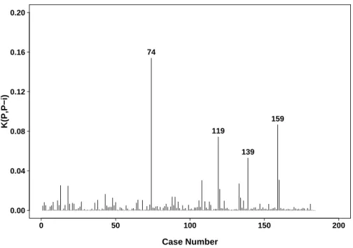
2.6.2 Stanford Heart Transplant Data . . . 35
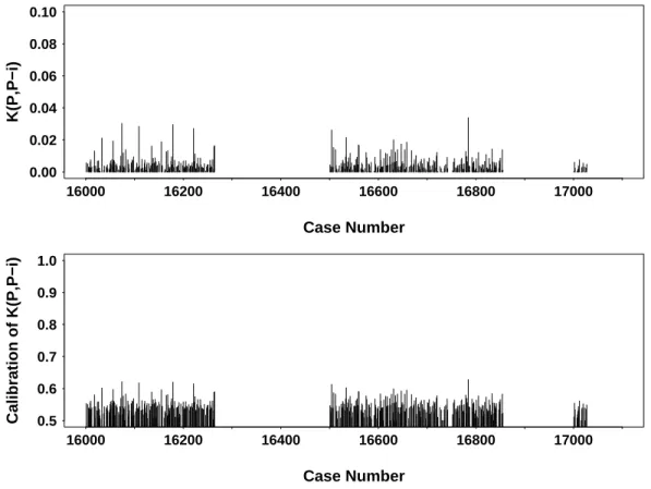
2.6.3 Melanoma Data . . . 37
2.7 Discussion . . . 40
3 BAYESIAN CASE INFLUENCE MEASURES AND THEIR APPLI-CATIONS 41 3.1 Introduction . . . 41
3.2 Bayesian Case Influence Measures . . . 43
3.2.1 Preliminaries . . . 43
3.2.2 Computation, Approximation and Calibration . . . 45
3.2.3 Deleting Large Numbers of Observations . . . 49
3.3 Applications to Model Assessment . . . 51
3.3.1 Model Complexity and Cross Validation . . . 51
3.3.2 Model Comparison Criterion . . . 55
3.4 Theoretical Examples . . . 56
3.4.1 Normal Linear Models . . . 57
3.4.2 Linear Mixed Models . . . 59
3.4.3 Generalized Linear Models . . . 61
3.4.4 Generalized Linear Mixed Models . . . 64
3.5.1 Generalized Linear Models: Binary Data . . . 66
3.5.2 Generalized Linear Mixed Models: Longitudinal Data . . . 72
3.6 Discussion . . . 75
4 SCALED COOK’S DISTANCE 77 4.1 Introduction . . . 77
4.2 Scaled Cook’s Distance . . . 79
4.2.1 Cook’s Distance . . . 79
4.2.2 Size Matters . . . 82
4.2.3 Scaled Cook’s Distance . . . 87
4.2.4 Conditional Scaled Cook’s Distance . . . 91
4.3 Illustrative Examples . . . 96
4.3.1 Finney Data . . . 96
4.3.2 Yale Infant Growth Data . . . 100
4.4 Discussion . . . 105
5 DISCUSSION 106
APPENDIX 108
A Proofs in Chap. 2 108
B Assumptions and Proofs in Chap. 3 111
C Assumptions in Chap. 4 121
LIST OF TABLES
2.1 Posterior means and standard deviations for the simulated data with
c=0.01 . . . 31
2.2 Case influence diagnostics for the simulated data . . . 33
2.3 Case influence diagnostics for the heart transplant data . . . 36
2.4 Case influence diagnostics for the E1690 data with c=0.01 . . . . 39
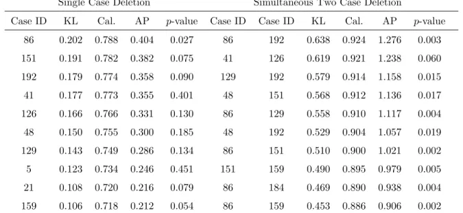
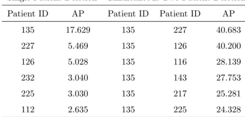
3.1 Case influence diagnostics based on the uniform improper prior forβ for Chapman data . . . 67
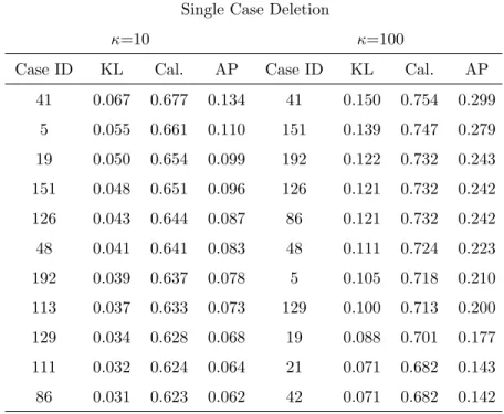
3.2 Case influence diagnostics based on the normal prior for βfor Chapman data . . . 68
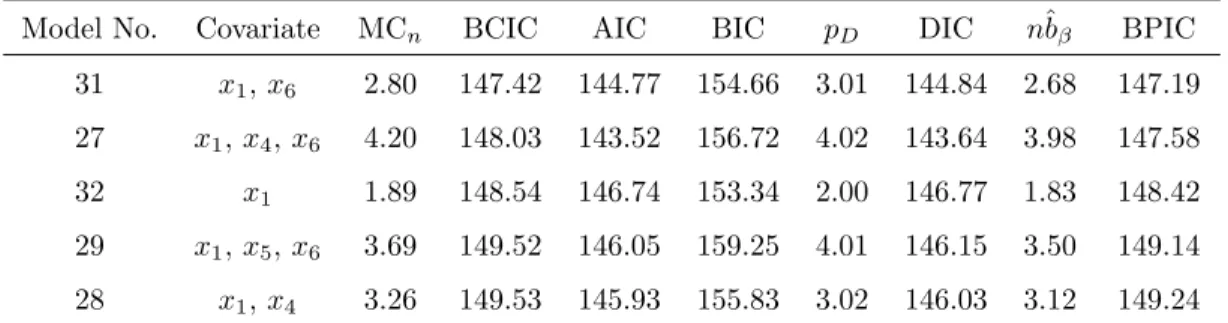
3.3 Information criteria for the top five models selected by BCIC based on the uniform improper prior for β for Chapman data . . . 70
3.4 Case influence diagnostics for the epileptic data . . . 73
LIST OF FIGURES
2.1 K(P, P−i) for the simulated data with c=0.01 . . . . 34
2.2 K(P, P−i) for the heart transplant data with c=0.01 . . . . 37
2.3 K(P, P−i) and calibration for the E1690 data with c=0.01 . . . 38
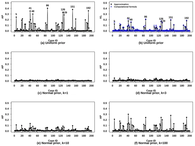
3.1 Case influence diagnostics, single case deletion for Chapman data . . . 69 3.2 Case influence diagnostics based on the uniform improper prior, two case
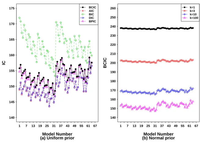
deletion for Chapman data . . . 70 3.3 Information criteria for Chapman data . . . 71 3.4 Index plot of case influence diagnostics for deleting a single patient at a
time for the epileptic data . . . 74 3.5 2-D scatter plot of case influence diagnostics for deleting two patients
simultaneously for the epileptic data . . . 76 4.1 Yale infant growth data: (a) the index plot of Cook’s distance; (b) cluster
size versus Cook’s distance. . . 81 4.2 Index plots for single case deletion for Finney data . . . 97 4.3 2-D scatter plots for simultaneous two case deletion for Finney data . . 98 4.4 3-D scatter plots for simultaneous three case deletion for Finney data . 99 4.5 Density plots in log10-scale for Finney data . . . 100 4.6 Index plots for single subject deletion with compound symmetry model
for Yale infant growth data . . . 102 4.7 Cluster size versus Cook’s distance for single subject deletion with
com-pound symmetry model for Yale infant growth data . . . 103 4.8 2-D scatter plots for simultaneous two subjects deletion with compound
LIST OF ABBREVIATIONS
AIC Akaike Information Criterion
ARMS Adaptive Rejection Metropolis Sampling BCIC Bayesian Case-influence Information Criterion BIC Bayesian Information Criterion
BPIC Bayesian Predictive Information Criterion CD Cook’s Distance
CPO Conditional Predictive Ordinate DIC Deviance Information Criterion K-L Kullback-Leibler
CHAPTER 1
INTRODUCTION AND
LITERATURE REVIEW
1.1
Introduction
Recently, Bayesian methodologies have been getting enormous attention in biomed-ical research due to the potential advantages of fitting a vast array of complex models posed by modern data. As the demand for Bayesian data analysis and modeling in-creases, we need good diagnostic methods for model assessment and selection. However, development of Bayesian influence diagnostic methods for parametric regression models pose both theoretical and computational challenges. Motivated by this, the first paper proposes Bayesian case influence diagnostics for complex survival models. We develop case deletion influence diagnostics for both the joint and marginal posterior distribu-tions based on the Kullback-Leibler divergence (K-L divergence) (Kullback and Leibler, 1951). We present a simplified expression for computing the K-L divergence between the posterior with the full data and the posterior based on single case deletion. In ad-dition, we investigate a theoretical connection between the proposed diagnostics based on the K-L divergence and Conditional Predictive Ordinate (CPO) (Gelfand et al., 1992; Geisser, 1993), as well as a connection between diagnostics based on Cox’s par-tial likelihood (Cox, 1975). The second paper introduces three types of Bayesian case influence measures based on case deletion, namely the φ-divergence, Cook’s posterior mode distance and Cook’s posterior mean distance to evaluate the effects of deleting a set of observations in general Bayesian parametric models. We examine the statis-tical properties of these three Bayesian case influence measures and their applications to identification of influential sets and model complexity. This complexity measure is related to the complexity terms in other information criteria such as the Akaike Infor-mation Criterion (AIC) (Akaike, 1973) and the Deviance InforInfor-mation Criterion (DIC) (Spiegelhalter et al., 2002), and the leave-k-out cross validation method (Stone, 1974, 1977, 2002; Geisser and Eddy, 1979).
longitudinal data) no rigorous approach has been developed to address a fundamental issue of Cook’s distance: “size matters”, that is Cook’s distance is a monotonic function of the size of the perturbation. This issue has been largely neglected in the literature. The size matters issue persists in any deletion diagnostic, because the size of the deletion diagnostic is associated with the size of the perturbation. The third paper develops a scaled version of Cook’s distance to address the size issue for deletion diagnostics in general parametric models. We use stochastic ordering to quantify the relationship between the size of perturbation and the amount of the perturbation on Cook’s distance. Our scaled Cook’s distance properly accounts for the size of a perturbation and the fitted model to the data.
The rest of this dissertation is organized as follows. The next section presents literature reviews of case influence measures and model assessment tools based on the criterion-based methods. Then we proceed to present each of the three papers: The first paper is presented in Chapter 2, and it develops Bayesian case influence diagnostics for survival models for both continuous survival time data and grouped survival data. The second paper is discussed in Chapter 3, and it proposes methods to evaluate the effects of deleting a set of observations in Bayesian regression models. These models include linear models, mixed models, generalized linear models and generalized linear mixed models. The third paper is discussed in Chapter 4, and it is dedicated to resolving the size issues for Cook’s distance in general parametric model.
1.2
Literature Review
1.2.1
Case Influence Measures
and local influence measures (Cook, 1977; Belsley et al., 1980; Cook and Weisberg, 1982; Cook, 1986). A general approach to influence analysis is studying the changes in the outcome or other aspects of an analysis caused by a small perturbations in the model. The most popular perturbation scheme is based on case deletion. In fact, case deletion is also a special case of perturbations in local influence analysis (Cook, 1986), which utilize the concept of normal curvature in differential geometry in assessing the local behavior of the likelihood displacement.
Two widely used case deletion measures for assessing case influence are Cook’s dis-tance (Cook, 1977) and likelihood displacement (Cook and Weisberg, 1982; Cook, 1986). Likelihood displacement and Cook’s distance have been used to detect influential ob-servations in various parametric and semiparametric models from the frequentist point of view (Cook and Weisberg, 1982; Thomas and Cook, 1989; Pettitt and Daud, 1989; Weissfeld, 1990; Escobar and Meeker, 1992). The likelihood displacement measures the effect of deleting one observation on overall model fit using the log-likelihood. Let β
be p×1 vector of the parameter of interest, ˆβ and ˆβ(i) be the parameter estimates, usually maximum likelihood estimates (MLE), with full data and with the ith case deleted data, respectively, and L(β) be the likelihood function for β. The likelihood displacement is defined by
LD(i) = 2{logL(ˆβ)−logL(ˆβ(i))}. (1.1)
For more about likelihood displacement, see Cook and Weisberg (1982), p182-183. Cook’s distance measures the effect of deleting one observation on a parameter estimate or a fitted value. The generalized Cook distance for β is defined by
where M is a positive definite weight matrix and M is often set as the Fisher infor-mation matrix. Since the seminal work of Cook (1977) on Cook’s distance in linear regression, considerable research has been devoted to developing deletion diagnostics including Cook’s distance for detecting influential observations (or clusters) in vari-ous statistical models including generalized linear models and the general linear model with correlated error (Cook, 1977; Cook and Weisberg, 1982; Chatterjee and Hadi, 1988; Andersen, 1992; Davison and Tsai, 1992; Wei, 1998; Haslett, 1999; Zhu et al., 2001; Fung et al., 2002). For instance, Preisser and Qaqish (1996) developed Cook’s distance for generalized estimating equations. Christensen et al. (1992) and Banerjee and Frees (1997) considered case deletion and subject deletion diagnostics, respectively. Zhu et al. (2001) developed deletion diagnostics for models with missing data.
In Bayesian analysis, considerable research has been devoted to developing single case influence measures for various specific statistical models including generalized lin-ear models, time series models, and survival models (Johnson and Geisser, 1983; John-son, 1985; Pettit, 1986; Kass et al., 1989; Carlin and PolJohn-son, 1991; Gelfand et al., 1992; Weiss and Cook, 1992; Geisser, 1993; Blyth, 1994; Peng and Dey, 1995; Weiss, 1996; Christensen, 1997; Bradlow and Zaslavsky, 1997). There are two distinct approaches in assessing influence of individual observations. One is assessing the influence on the posterior distribution and other is assessing the influence with regard to the predictive distribution. For those two approaches, a common way of assessing the influence of an observation on model fit is through case deletion.
discrepancy between the posterior distributions with and without a particular case. Various forms of φ(·) have been considered in the literature (Weiss, 1996; Weiss and Cook, 1992; Kass et al., 1989; Blyth, 1994), which includeL1−distance,χ2−divergence
and Kullback-Leibler divergence (K-L divergence). A large value of the φ−divergence for the ith case implies more influence of the ith case on estimation, hypothesis test-ing, and model fit. Many researchers have been interested in developing case influence diagnostics using theφ−divergence, especially K-L divergence, under various paramet-ric models (Johnson and Geisser, 1985; Pettit, 1986; Carlin and Polson, 1991; Weiss and Cook, 1992; Peng and Dey, 1995; Weiss, 1996; Christensen, 1997; Weiss and Cho, 1998). Pettit (1986) suggested the use of the K-L divergence in detecting influential observations in his review of Bayesian diagnostics. Carlin and Polson (1991) proposed an expected utility approach using the K-L divergence as a utility function to define the influence of a set of observations in a parametric modeling framework, considering the normal linear model and mixed models. Weiss and Cook (1992) introduced the K-L divergence to assess the divergence between posteriors in the context of case deletion in generalized linear models. Peng and Dey (1995) also developed a Bayesian diag-nostic measure using general divergence measures including the K-L divergence on the posterior distribution and applied this measure to several regression models, such as a nonlinear model. Weiss (1996) and Weiss and Cho (1998) proposed assessing the influ-ence of case deletion using model perturbations as well as establishing its relationship to the K-L divergence and CPO. Bayesian influence measures for assessing marginal posterior distributions have also been developed for the multivariate linear model and normal random effects models (Johnson and Geisser, 1985; Weiss and Cho, 1998).
1.2.2
Criterion-Based Model Assessment
framework, information criteria (IC) are fundamental criteria for model comparisons, which incorporate measures of fit and complexity for model choice. Typically, deviance statistics are used for the measure of fit, and the number of parameters or degrees of freedom of estimators are used for the complexity of a model.
Considerable research has been devoted to model comparison and evaluation using the concepts of information criteria in both the frequentist and Bayesian point of views (Akaike, 1973; Takeuchi, 1976; Schwarz, 1978; Murata et al., 1994; Konishi and Kita-gawa, 1996; Spiegelhalter et al., 2002; Ando, 2007), in which they incorporate different complexity terms for model choice. Akaike (1973) proposed the Akaike Information Criterion (AIC) which is defined by AIC = −2 log{p(y|θˆ)}+ 2p, where p is the num-ber of parameters and ˆθ is the MLE of θ. The Takeuchi Information Criterion (TIC) (Takeuchi, 1976) and Generalized Information Criterion (GIC) (Konishi and Kitagawa, 1996) are generalizations of AIC which relax the following assumptions: (i) a specified parametric family of distributions include the true model; and (ii) a model is “esti-mated” by its MLE. TIC relaxed assumption (i) and GIC relaxed both (i) and (ii). Murata et al. (1994) proposed the Network Information Criterion (NIC) as a general-ization of AIC for determining the optimal number of parameters in neural networks. Schwarz (1978) adopted Bayesian argument in the development of the Bayesian Infor-mation Criterion (BIC), which is defined by BIC = −2 log{p(y|θˆ)}+plog(n), where n is the number of observations in the dataset. The Deviance Information Criterion (DIC) (Spiegelhalter et al., 2002) is defined by the posterior mean of the deviance as a Bayesian measure of fit and the effective number of parameters as the complexity component. DIC is given by DIC = −2Eθ|Y[log{p(y|θ)}] + pD, where Eθ|Y[·] is the
expectation with respect to the posterior distribution,p(θ|y). The effective number of parameters, pD is defined by pD = Eθ|Y[−2 log{p(y|θ)}] + 2 log{p(y|θ˜)}, where ˜θ is
Predictive Information Criterion (BPIC) was proposed by Ando (2007) as an estima-tor of the posterior mean of the expected log-likelihood of the predictive distribution. BPIC is defined as BPIC = −2Eθ|Y[log{p(y|θ)}] + 2nˆbθ, where ˆbθ is the estimated
asymptotic bias of the predictive discrepancy measures. For more details about ˆbθ, see
CHAPTER 2
BAYESIAN CASE INFLUENCE
DIAGNOSTICS FOR SURVIVAL
MODELS
2.1
Introduction
In Bayesian analysis, considerable research has been done for developing case influence diagnostics using the K-L divergence under various parametric models (Johnson and Geisser, 1985; Pettit, 1986; Carlin and Polson, 1991; Weiss and Cook, 1992; Weiss, 1996; Weiss and Cho, 1998). Despite the extensive literature on Bayesian diagnostic methods for parametric models, very little has been developed for semiparametric mod-els, including survival models. Due to the potential advantages of fitting a vast array of complex survival models posed by modern survival data, semiparametirc Bayesian methodologies in survival analysis have been getting enormous attention in biomedical research. Bayesian case influence diagnostics for survival models pose both theoretical and computational challenges, which are discussed here.
2.6.1 and 2.6.3, respectively.
The rest of this paper is organized as follows. In Section 2.2, we introduce Bayesian case influence diagnostics based on the K-L divergence. In Sections 2.3 and 2.4, we derive case influence diagnostics for the Cox model and Cox frailty model with a gamma process prior. In Section 2.5, we present case influence diagnostics for the Cox model with a beta process prior. In Section 2.6, we examine the performance of the influence diagnostics using simulated data, the Stanford Heart Transplant data and the E1690 trial. We conclude the paper with some discussion in Section 2.7.
2.2
The Proposed Method
2.2.1
General Development
Let D be full data and D−i be the data with the ith case deleted. Let L(β|D)
denotes the likelihood based on the full data and L(β|D−i) denotes the likelihood
based on the data without the ith case. The posterior distributions for the the full data and the ith case deleted can be defined as p(β|D) ∝ L(β|D)π(β) and p(β|D−i) ∝ L(β|D−i)π(β), respectively, where π(β) is the prior distribution of β.
A typical choice of π(β) is a Np(µ0,Σ0) distribution or a uniform improper prior.
LetK(P, P−i) denote the K-L divergence between P and P−i, where P denotes the
posterior distribution of β for the full data, and P−i denotes the posterior distribution
of β without the ith case. Specifically,
K(P, P−i) =
Z
p(β|D) log
½
p(β|D) p(β|D−i)
¾
dβ. (2.1)
K(P, P−i) thus measures the effect of deleting the ith case from the full data on the
joint posterior distribution of β. Note that K(P, P−i) 6= K(P−i, P) in general. After
K(P, P−i) as follows:
K(P, P−i) = logEβ
·
L(β|D−i)
L(β|D)
¯ ¯ ¯ ¯D
¸
+Eβ
·
log
½
L(β|D) L(β|D−i)
¾¯¯ ¯ ¯D
¸
, (2.2)
whereEβ[·|D] represents the expectation with respect to the joint posterior distribution
of β given D. Equation (2.2) enables us to compute K(P, P−i) for i= 1,· · · , n, using
only samples from the full data joint posterior distribution ofβ. Therefore, (2.2) implies that we completely avoid sampling from p(β|D−i) for the computation of K(P, P−i),
and this saves us enormous computational time and effort.
Now suppose that interest lies in assessing the influence of theith case on the subset
β1 of the parameter vector β = (β1,β2). Weiss and Cho (1998), Weiss (1996), and
Weiss and Cook (1992) pointed out that if the goal of an analysis is to assess the influence of the ith case on the marginal posterior distribution of β1, then using the
joint posterior of (β1,β2) to assess this influence may overstate the influence. Hence, in
these settings, we need to consider the influence of a case using the marginal posterior distribution ofβ1.
We can express the marginal influence diagnostics of Weiss and Cho (1998) based on directed the K-L divergence as
K(P1, P1,−i) =
Z
p1(β1|D) log
½
p1(β1|D)
p1(β1|D−i)
¾
dβ1, (2.3)
where p1(β1|D) =
R
p(β1,β2|D)dβ2. The marginal K-L divergence, K(P1, P1,−i), in
(2.3) measures the effect of deleting the ith case from the full data on the marginal posterior distribution of β1. Using similar derivations as in (2.2), we can obtain a
simplified expression forK(P1, P1,−i) as follows:
K(P1, P1,−i) = logEβ
·
L(β|D−i)
L(β|D)
¯ ¯ ¯ ¯D
¸
−Eβ1
·
log
Z
L(β|D−i)
L(β|D) p(β2|β1, D)dβ2
where p(β2|β1, D)=p(β1,β2|D)/
R
p(β1,β2|D)dβ2 and
Z
L(β|D−i)
L(β|D) p(β2|β1, D)dβ2 can be evaluated as Eβ2
·
L(β|D−i)
L(β|D)
¯ ¯ ¯ ¯β1, D
¸
.
Following McCulloch (1989), calibration of K(P, P−i) can be done by solving forpi
such that K(P, P−i)=K(B(0.5), B(pi))=−log{4pi(1−pi)}/2, where B(p) denotes the
Bernuolli distribution with success probabilityp. This implies that describing outcomes usingp(β|D−i) instead ofp(β|D) is compatible with describing an unobserved event as
having probability pi when the correct probability is 0.5. After calculating K(P, P−i)
from (2.2), we can compute pi using pi = 0.5
h
1 +p1−exp{−2K(P, P−i)}
i
. This equation implies that 0.5 ≤ pi ≤ 1. pi À 0.5 implies that the ith case is influential,
because deleting the ith case changes the posterior distribution as much as describing an observed event as having probability pi when the correct probability is 0.5. In this
paper, we use pi as the calibration ofK(P, P−i) in all of the examples.
2.2.2
Independence Model
As an illustration, we consider the proposed diagnostic for the independence model. Suppose that given β, yi, i = 1,2,· · · , n are independent response variables, not
subject to censoring. Then the full data likelihood is L(β|D) = Qnk=1f(yk|β),
where f(yk|β) is the density of yk and the likelihood without the ith observation is
L(β|D−i) =
Qn
k=1,k6=if(yk|β). Therefore, L(β|D)/L(β|D−i)=f(yi|β) and the CPO is
given by CP Oi = [Eβ[{f(yi|β)}−1|D]]−1 (Gelfand et al., 1992).
Using (2.2) and the above results, we can therefore show that
K(P, P−i) = logEβ[{f(yi|β)}−1|D] +Eβ[log{f(yi|β)}|D]
= −log(CP Oi) +Eβ[log{f(yi|β)}|D]. (2.5)
ith case on the marginal posterior distribution of β1 and its connection with CPO
as follows:
K(P1, P1,−i) = logEβ[{f(yi|β)}−1|D]
− Z
p(β1|D) log[
Z
{f(yi|β)}−1p(β2|β1, D)dβ2]dβ1
= −log(CP Oi)−Eβ1[log
Z
{f(yi|β)}−1p(β2|β1, D)dβ2|D], (2.6)
wherep(β2|β1, D) =p(β1,β2|D)/
R
p(β1,β2|D)dβ2 and
R
{f(yi|β)}−1p(β2|β1, D)dβ2
can be evaluated as Eβ2[{f(yi|β)}−1|β1, D]. Since (2.2), (2.4), (2.5) and (2.6) are
expressed as posterior expectations with respect to the full data posterior distribution, they can be easily calculated using only MCMC samples from the full data posterior distribution ofβ.
2.3
Cox Model with Gamma Process Prior
2.3.1
Model
In the Cox proportional hazards model (Cox, 1972), the gamma process is a very com-monly used nonparametric prior process for the cumulative baseline hazard (Kalbfleisch, 1978). The full data is denoted as D = {y,δ,X}, where y = (y1, y2,· · · , yn)0
de-notes the observed survival times, where yi may be right censored. We assume that
the survival times are all distinct and ordered, i.e., 0 < y1 < y2 < · · · < yn < ∞.
δ = (δ1, δ2,· · · , δn)0 is an indicator vector with δi = 1 if the ith subject failed, and
δi = 0 if the ith subject was right censored. Also, X is an n×p matrix of covariates
withith rowx0
i, andD−i ={y−i,δ−i,X−i}denotes the data with theith subject, (i.e.,
(yi, δi,x0i)) deleted fromD. The hazard function is given byh(yi|xi) =h0(yi) exp(x0iβ),
baseline hazard function.
Under the Cox model, the joint probability of the survival of n subjects is given by
P(Y >y|β,X, H0) = exp (
−
n
X
k=1
H0(yk) exp(x0kβ)
)
, (2.7)
where H0(y) is the cumulative baseline hazard (Ibrahim et al., 2001a). We take H0 ∼
GP(cH∗(·), c), where GP denotes gamma process, H∗(y) is a known differentiable parametric function which represents a parametric guess for the cumulative baseline hazard H0(y), and c ≥ 0 is a confidence parameter. H∗(y) is thus the mean of the
process. Letting hk = H0(yk)−H0(yk−1), we take hk ∼ Gamma(ch0k, c), the hk’s are
independent, where h0k = H∗(yk)−H∗(yk−1) and Gamma(α, λ) denotes the gamma
distribution with meanα/λ (α >0 and λ >0).
The marginal likelihood function ofβcan now be written as follows (Ibrahim et al., 2001a; Sinha et al., 2003) :
L(β|D) =
n
Y
k=1
Lk(β|D) (2.8)
=
n
Y
k=1
exp
·
cH∗(yk) log
½
1− exp(x
0
kβ)
c+Ak
¾¸ ·
−ch∗(yk) log
½
1− exp(x
0
kβ)
c+Ak
¾¸δk
,
where h∗(y) = d
dyH∗(y), Ak =
P
l∈R(yk)exp(x
0
lβ), and R(yk) = {l : yl ≥yk} is the set
of subjects at risk at timeyk.
We now derive the likelihood function without the ith subject. If yk < yi then
the risk set at time yk involves the ith subject, otherwise, the risk set at yk does not
involve the ith subject. Therefore, after deleting the ith subject, the risk set changes toR(yk) ={l :yl ≥yk, l 6=i} for k < i. As the risk set changes, the corresponding Ak
in the denominators of (2.8) changes toAk−exp(x0iβ) for k < i, whereas fork > i, the
function without theith subject is given by
L(β|D−i) = i−1 Y
k=1
Lk,−i(β|D) n
Y
k=i+1
Lk(β|D), (2.9)
where
Lk,−i(β|D) = exp
·
cH∗(y
k) log
½
1− exp(x0kβ)
c+Ak−exp(x0iβ)
¾¸
× ·
−ch∗(yk) log
½
1− exp(x
0
kβ)
c+Ak−exp(x0iβ)
¾¸δk
,
Lk(β|D) = exp
·
cH∗(y
k) log
½
1−exp(x0kβ)
c+Ak
¾¸ ·
−ch∗(y
k) log
½
1− exp(x0kβ)
c+Ak
¾¸δk
.
The posterior distributions based on the full data and the data without theith subject are thus given by p(β|D)∝L(β|D)π(β) and p(β|D−i)∝L(β|D−i)π(β), respectively.
2.3.2
Diagnostic Measures
For the Cox model in general, the likelihood function cannot be written as a product of n independent terms because the risk set for the kth subject involves observations other than thekth subject. Because of this dependency, we use (2.8) for the likelihood function. Another advantage of (2.8) is its computational feasibility. Since the hazard, hk, has been integrated out from (2.8), (2.8) is only a function ofβ. Therefore, sampling
the hk’s is not necessary for Bayesian inference and diagnostics, and thus only samples
from the posterior distribution of β are needed.
After some algebra, the ratio of likelihoods for the full data and the data without theith subject can be written asL(β|D)/L(β|D−i)=gi(β)Li(β|D). Thus, we can get a
simplified expression for computing the influence of theith subject on the joint posterior distribution ofβ as follows:
K(P, P−i) = logEβ[{gi(β)Li(β|D)}−1|D] +Eβ[log{gi(β)Li(β|D)}|D] (2.10)
where
Li(β|D) = exp
·
cH∗(y
i) log
½
1− exp(x0iβ)
c+Ai
¾¸ ·
−ch∗(y
i) log
½
1− exp(x0iβ)
c+Ai
¾¸δi
, (2.11) gi(β) =
Qi−1
k=1Lk(β|D)/
Qi−1
k=1Lk,−i(β|D), which can be simplified as
gi(β) =
i−1 Y
k=1 ·
1− exp(x
0
kβ)
c+Ak
¸cH∗(y
k)·
−log
½
1−exp(x
0
kβ)
c+Ak
¾¸δk
i−1 Y
k=1 ·
1− exp(x0kβ)
c+Ak−exp(x0iβ)
¸cH∗(y
k)·
−log
½
1− exp(x0kβ)
c+Ak−exp(x0iβ)
¾¸δk .
(2.12) In addition, CP Oi can be written as,
CP Oi =
Eβ[{gi(β)}−1|D]
Eβ[{gi(β)Li(β|D)}−1|D]
. (2.13)
Since (2.10) is expressed as a posterior expectation with respect to the full data, computation of (2.10) can be done using MCMC samples from the full data posterior p(β|D). The samples from p(β|D) can be easily obtained using Adaptive Rejection Metropolis Sampling (ARMS, Gilks et al. (1995)) within Gibbs. Specifically, we have
K(P, P−i) = log
" 1 J J X j=1
{gi(β(j))Li(β(j)|D)}−1
# + 1 J J X j=1
log{gi(β(j))Li(β(j)|D)} ,
(2.14) and
CP Oi =
1 J
J
X
j=1
{gi(β(j))}−1
1 J
J
X
j=1
{gi(β(j))Li(β(j)|D)}−1
, (2.15)
jth Gibbs sample, j = 1,· · · , J. Similarly, we obtain
K(P1, P1,−i)
= logEβ[{gi(β)Li(β|D)}−1|D]−Eβ1[log
Z
{gi(β)Li(β|D)}−1p(β2|β1, D)dβ2|D] (2.16)
=−log(CP Oi) + logEβ[{gi(β)}−1|D]−Eβ1[log
Z
{gi(β)Li(β|D)}−1p(β2|β1, D)dβ2|D].
Monte Carlo evaluation ofEβ1[log
R
{gi(β)Li(β|D)}−1p(β2|β1, D)dβ2|D] in (2.16) can
be obtained using the following steps:
Step 1. We use Gibbs sampling to obtain the samples β(j) = (β
1(j),β2(j)) for j =
1,· · · , J from p(β|D) and record (β1(1),· · · ,β1(J)) as J Gibbs samples from the
marginal posterior of β1, p(β1|D).
Step 2. We use Gibbs sampling to obtain the samples β(r) = (β1(r),β2(r)) for r =
1,· · · , R fromp(β|D) and record (β2(1),· · · ,β2(R)) as RGibbs samples from the
marginal posterior of β2 given β1, p(β2|β1, D).
Step 3. For each β1(j), use β2(r) as nested Gibbs samples from p(β2|β1(j), D) to get
the Monte Carlo approximation ofEβ1[log
R
{gi(β)Li(β|D)}−1p(β2|β1, D)dβ2|D]
as 1
J
PJ
j=1log[R1
PR
r=1{gi(β1(j),β2(r)), Li(β1(j),β2(r)|D)}−1].
Note that the Gibbs samples in the first and second steps need to be sampled indepen-dently. Now, we can get the MCMC approximation of (2.16) as
K(P1, P1,−i) = log
"
1 J
J
X
j=1 n
gi(β1(j),β2(j))Li(β1(j),β2(j)|D)
o−1#
(2.17)
−1
J
J
X
j=1
log
"
1 R
R
X
r=1 n
gi(β1(j),β2(r))Li(β1(j),β2(r)|D)
o−1#
.
orK(P1, P1,−i) across subjects to identify influential cases.
Since K(P, P−i) measures the effect of deleting the ith case on the joint posterior
distribution ofβ, it can be viewed as a Bayesian analogue of the likelihood displacement (LD), as discussed in Cook (1986). Specifically, for the Cox model, K(P, P−i) is
com-parable to the likelihood displacement based on partial likelihood, which is available in Statistical Analysis Systems (SAS) version 9.1.3. For more on likelihood displacement for the Cox model, see Pettitt and Daud (1989). In addition, a limiting expression forK(P, P−i) based on model (2.8) provides a method for computing K(P, P−i) under
Cox’s partial likelihood.
2.3.3
Relationship to Partial Likelihood
In this subsection, we derive a limiting expression for K(P, P−i) based on model (2.8)
in Section 2.3. This result provides a method for computing K(P, P−i) under Cox’s
partial likelihood. Kalbfleisch (1978) and Sinha et al. (2003) showed that the partial likelihood defined by Cox (1975) can be obtained as a limiting case of the marginal posterior for β in the Cox model with continuous time survival data under a gamma process prior for the cumulative baseline hazard. The partial likelihood can be written as (Sinha et al., 2003)
lim
c→0
L(β|D) cPnk=1δk(−logc)δnQn
k=1{h∗(yk)}δk
=
n
Y
k=1 ½
exp(x0
kβ)
Ak
¾δk
. (2.18)
Therefore,
lim
c→0
Li(β|D)
cδi{h∗(yi)}δi = ½
exp(x0
iβ)
Ai
¾δi
, for i= 1,· · · , n−1, (2.19)
and
lim
c→0
Ln(β|D)
cδn(−logc)δn{h∗(y
n)}δn
=
½
exp(x0
nβ)
An
¾δn
Using similar ideas and extensions of the proofs of (2.18), we can derive the limiting expression ofgi(β) as c→0. Since An−1−exp(x0nβ) = exp(x0n−1β), we have
lim
c→0gi(β) =
i−1 Y
k=1 ½
exp(x0
kβ)
Ak
¾δk
i−1 Y
k=1 ½
exp(x0
kβ)
Ak−exp(x0iβ)
¾δk, for i= 1,· · ·, n−1, (2.21)
and
lim
c→0(−logc)
δn−1g
i(β) = i−1 Y
k=1 ½
exp(x0
kβ)
Ak
¾δk
i−1 Y
k=1 ½
exp(x0
kβ)
Ak−exp(x0iβ)
¾δk, for i=n. (2.22)
Using the above results, it follows that
lim
c→0K(P, P−i) = limc→0 £
logEβ[{gi(β)Li(β|D)}−1|D] +Eβ[log{gi(β)Li(β|D)}|D]
¤
(2.23) = logEβ[lim
c→0{αigi(β)Li(β|D)}
−1|D] +E
β[log{lim
c→0αigi(β)Li(β|D)}|D],
where
αi =
1
cδi{h∗(yi)}δi for i= 1,· · · , n−1,
(−logc)δn−1
cδn{h∗(yn)}δn(−logc)δn for i=n.
(2.24)
Hence, we can obtain
K∗(P, P−i)≡lim
c→0K(P, P−i) = logEβ[{Mi(β)}
−1|D] +E
β[log{Mi(β)}|D], (2.25)
where
Mi(β) = i−1 Y
k=1 ½
exp(x0
kβ)
Ak
¾δk½
exp(x0
iβ)
Ai
¾δi
i−1 Y
k=1 ½
exp(x0
kβ)
Ak−exp(x0iβ)
¾δk . (2.26)
Thus, we can computeK∗(P, P
(2.8) in Section 2.3.
2.4
Frailty Model with Gamma Process Prior
2.4.1
Model
In survival analysis, the hazard function for each individual may depend on a set of frailties representing unobservable risk factors. In this section, we extend the results of Sinha et al. (2003) to the proportional hazards frailty model and develop Bayesian case deletion diagnostic measures.
Let yij denote the survival times and xij denotes the p×1 covariate vector for the
jth subject in theith cluster fori= 1,2,· · · , nandj = 1,2,· · · , mi. The total number
of subjects isN =Pni=1mi and δij is an indicator withδij = 1 if thejth subject in the
ith cluster failed andδij = 0 otherwise. The hazard function is given byh(yij|wi,xij) =
h0(yij)wiexp(x0ijβ), whereβis thep×1 vector of unknown regression coefficients,h0(.)
is an unknown baseline hazard function, and wi is the frailty term for the ith cluster.
To extend the results of Sinha et al. (2003), we first rearrange the data as follows. Let D = {X,y,δ,w} denote the complete data. We assume that the survival times,
y = (y1, y2,· · · , yN)0, are all distinct and ordered as 0 < y1 < y2 < · · · < yN < ∞,
X is an N ×p matrix of covariates with kth rowx0
k, δ = (δ1, δ2,· · · , δN)0 is the right
censoring indicator vector, andw= (w(1), w(2),· · · , w(N))0 is the frailty vector according
to (y1, y2,· · · , yN). Thus, h(yk|w(k),xk) = h0(yk)w(k)exp(x0kβ), k = 1,2,· · · , N, and
assuming a gamma process prior for H0(y) as in Section 2.3.1, the likelihood function
can be obtained as
L(β|D) =
N
Y
k=1
Lk(β|D) (2.27)
=
N
Y
k=1
exp
·
cH∗(y
k) log
½
1−w(k)exp(x
0
kβ)
c+Awk
¾¸ ·
−ch∗(y
k) log
½
1−w(k)exp(x
0
kβ)
c+Awk
¾¸δk
where h∗(y) = d
dyH∗(y),Awk =
P
l∈R(yk)w(l)exp(x
0
lβ) and R(yk) ={l :yl ≥yk} is the
set of subjects at risk at time yk.
Now, we consider the data with the ith subject deleted. If the ith subject is the only observation in a cluster (mi = 1), the frailty term for that cluster is deleted along
with the deletion of theith subject. Otherwise, the frailty term for the cluster remains. Therefore, we denote the data with theith subject deleted asD−i = (y−i,δ−i,X−i,w)
for mi ≥ 2 and D−i = (y−i,δ−i,X−i,w(−i)) for mi = 1. Furthermore, let Dobs =
{X,y,δ} denote the observed data and Dobs,−i ={X−i,y−i,δ−i} denote the observed
data with theith subject deleted. Because of the change in the risk set with the deletion of the ith subject, Awk in the denominators of (2.27) becomes Awk −wiexp(x0iβ) for
k < i and remains as Awk for k > i. Thus,
L(β|D−i) = i−1 Y
k=1
Lk,−i(β|D) N
Y
k=i+1
Lk(β|D)
=
i−1 Y
k=1
exp
·
cH∗(yk) log
½
1− w(k)exp(x
0
kβ)
c+Awk−w(i)exp(x0iβ)
¾¸
× ·
−ch∗(y
k) log
½
1− w(k)exp(x
0
kβ)
c+Awk−w(i)exp(x0iβ)
¾¸δk
(2.28)
×
N
Y
k=i+1
exp
·
cH∗(yk) log
½
1− w(k)exp(x
0
kβ)
c+Awk
¾¸ ·
−ch∗(yk) log
½
1− w(k)exp(x
0
kβ)
c+Awk
¾¸δk
.
We assume that β and w are independent a priori and π(w) =Qnj=1π(wj), where
the wj’s are i.i.d. gamma random variables with mean 1. The posterior distribution
for the observed data is p(β,w|Dobs) ∝ L(β|D)π(w)π(β). The posterior distribution
for the observed data with theith subject deleted is given by
p(β,w|Dobs,−i)∝
L(β|D−i)π(w)π(β) for mi ≥2,
L(β|D−i)
Qn
j=1,j6=iπ(wj)π(β) for mi = 1.
2.4.2
Diagnostic Measures
For the computation ofK(P, P−i), we assume that there are at least two subjects in each
cluster (mi ≥2). The influence of the ith subject on the joint posterior distribution of
β is given by
K(P, P−i) =
Z Z
p(β,w|Dobs) log
½
p(β,w|Dobs)
p(β,w|Dobs,−i)
¾
dβdw. (2.30)
If we denote the ratio of likelihoods with full data and data without theith subject as L(β|D)/L(β|D−i) = gi(β,w)Li(β|D), K(P, P−i) can be computed as follows:
K(P, P−i) = log[Eβ,w[{gi(β,w)Li(β|D)}−1|Dobs]] +Eβ,w[log{gi(β,w)Li(β|D)}|Dobs]
= −log(CP Oi) +Eβ,w[logLi(β|D)|Dobs]
+ log[Eβ,w[{gi(β,w)}−1|Dobs]] +Eβ,w[loggi(β,w)|Dobs], (2.31)
where Eβ,w[ · |Dobs] is the expectation with respect to the joint posterior of (β,w)
given Dobs. The corresponding Li(β|D), gi(β,w) and CP Oi can be written as
Li(β|D) = (2.32)
exp
·
cH∗(y
k) log
½
1− w(k)exp(x
0
kβ)
c+Awk
¾¸ ·
−ch∗(y
k) log
½
1− w(k)exp(x
0
kβ)
c+Awk
¾¸δk
,
gi(β,w) = (2.33)
i−1 Y
k=1 ·
1− w(k)exp(x
0
kβ)
c+Awk
¸cH∗(y
k)·
−log
½
1− w(k)exp(x
0
kβ)
c+Awk
¾¸δk
i−1 Y
k=1 ·
1− w(k)exp(x
0
kβ)
c+Awk−w(i)exp(x0iβ)
¸cH∗(y
k)·
−log
½
1− w(k)exp(x
0
kβ)
c+Awk−w(i)exp(x0iβ)
and
CP Oi =
Eβ,w[{gi(β,w)}−1|Dobs]
Eβ,w[{gi(β,w)Li(β|D)}−1|Dobs]
. (2.34)
The computation of (2.31) can be accomplished using MCMC samples from p(β,w|Dobs). To obtain samples from p(β,w|Dobs), we perform ARMS within Gibbs
using the full conditional distributions (i)p(β|w, Dobs) and (ii) p(w|β, Dobs).
In assessing the influence of case deletion on β1 of β= (β1,β2), we define
K(P1, P1,−i) =
Z Z
p1(β1,w|Dobs) log
½
p1(β1,w|Dobs)
p1(β1,w|Dobs,−i)
¾
dβ1dw, (2.35)
where
p1(β1,w|Dobs) =
Z
p(β1,β2,w|Dobs)dβ2
p1(β1,w|Dobs,−i) =
Z
p(β1,β2,w|Dobs,−i)dβ2.
A computational formula for K(P1, P1,−i) is therefore given by
K(P1, P1,−i) = log[Eβ,w[{gi(β,w)Li(β|D)}−1|Dobs]] (2.36)
−Eβ1,w[log
Z
{gi(β,w)Li(β|D)}−1p(β2|β1,w, Dobs)dβ2|Dobs]
= −log(CP Oi) + log[Eβ,w[{gi(β,w)}−1|Dobs]]
−Eβ1,w[log
Z
{gi(β,w)Li(β|D)}−1p(β2|β1,w, Dobs)dβ2|Dobs],
where p(β2|β1,w, Dobs) = p(β1,β2,w|Dobs)/
R
p(β1,β2,w|Dobs)dβ2. The
computa-tion of (2.36) can also be carried using MCMC samples from p(β,w|Dobs).
2.4.3
Relationship to Partial Likelihood
distribution ofβbased on the frailty model discussed in Section 2.4.1. For the likelihood given by (2.27), we can show that
lim
c→0
L(β,w|D) cPNk=1δk(−logc)δNQN
k=1{h∗(yk)}δk '
N
Y
k=1 ½
w(k)exp(x0kβ)
Awk
¾δk
. (2.37)
We see that the right-hand side of (2.37) is equal to the frailty model based on Cox’s partial likelihood (Sargent, 1998).
Using a similar method as for proving (2.25), it can be shown that
lim
c→0K(P, P−i) = logEβ,w[{Mi(β,w)}
−1|D
obs] +Eβ,w[logMi(β,w)|Dobs], (2.38)
where
Mi(β,w) = i−1 Y
k=1 ½
w(k)exp(x0kβ)
Awk
¾δk½
w(i)exp(x0iβ)
Awi
¾δi
i−1 Y
k=1 ½
w(k)exp(x0kβ)
Awk−w(i)exp(x0iβ)
¾δk . (2.39)
Therefore, we can compute K(P, P−i) for the frailty model based on partial likelihood
using MCMC samples from thep(β,w|Dobs) implied by (2.27).
2.5
Cox Model with Beta Process Prior
2.5.1
Model
The actual survival time is often unknown in medical studies. However, we can obtain the information whether the subject is failed or censored in a given interval. In this case, the data is available as grouped within the intervals and called grouped survival data. We construct a finite partition of the time axis, 0 < s1 < s2 < · · · < sJ, with
sJ > yi for i = 1,2,· · · , n. Thus, we have J disjoint intervals and let Ij = (sj−1, sj].
(X,Rj,Dj :j = 1,2,· · · , J) as full data, where Rj is the risk set andDj is the failure
set of thejth interval Ij. To define the data with theith subject deleted from the full
data, we assume that the ith subject is in the ath interval, Ia = (sa−1, sa]. And we
denoteD−i = (X,R−ai,D−ai,Rj,Dj :j = 1,· · · , a−1, a+ 1,· · · , J) as the data without
the ith subject, where R−i
a is the risk set and D−ai is the failure set of the ath interval
without the ith subject. We also assume that the censoring indicator for the deleted subject is known.
To model the grouped survival data, we consider the discretized beta process (Hjort, 1990; Sinha, 1997) with a grouped data likelihood (Ibrahim et al., 2001a). Let hj be
the discretized baseline hazard rate in the interval Ij = (sj−1, sj], j = 1,2,· · · , J
and we specify independent beta priors for the hj’s. Specifically, we take hj ∼
Beta(c0kα0k, c0k(1−α0k)), and hj are independent for j = 1,2,· · · , J. The likelihood
is given by (Ibrahim et al., 2001a)
L(β,h|D) =
J
Y
j=1
Lj(β,h|D)
=
J
Y
j=1
Y
k∈Rj−Dj
(1−hj)exp(x
0
kβ) Y
l∈Dj n
1−(1−hj)exp(x
0
lβ) o
, (2.40)
whereh= (h1, h2,· · · , hJ)0.
After deleting theith subject, the risk set and failure set of theath interval change. Since the risk set of the ath interval always contains theith subject, it becomes Ra−
{ith subject} after deleting the ith subject. On the other hand, the failure set of the ath interval contains the ith subject only if the survival time is observed from the failure (event). Therefore, the failure set becomesDa− {ith subject}, if theith subject
without theith subject (ith subject∈ Ia) is given by
L(β,h|D−i) = J
Y
j=1,j6=a
Lj(β,h|D)La(β,h|D−i) (2.41)
=
J
Y
j=1
Lj(β,h|D)
h
(1−δi)(1−ha)exp(x
0
iβ)+δ
i
n
1−(1−ha)exp(x
0
iβ) oi−1
,
where δi is the indicator for the ith subject having 1 for failure and 0 for censoring.
La(β,h|D−i) is the likelihood for the ath interval without theith subject and given by
La(β,h|D−i) = La(β,h|D)
h
(1−δi)(1−ha)exp(x
0
iβ)+δ
i
n
1−(1−ha)exp(x
0
iβ) oi−1
. (2.42) A typical prior distribution for β is a Np(µ0,Σ0), which is independent of h. The
posterior distributions for full data and data without theith subject are given by
p(β,h|D) =L(β,h|D)π(h)π(β)/
Z Z
L(β,h|D)π(h)π(β)dhdβ ,
and
p(β,h|D−i) =L(β,h|D−i)π(h)π(β)/
Z Z
L(β,h|D−i)π(h)π(β)dhdβ. (2.43)
Sampling from the joint posterior distribution of (β,h), p(β,h|D), can be done by using transformation qj = −log(1 −hj), j = 1,2,· · · , J and exponential auxiliary
2.5.2
Diagnostic Measures
We define CPO statistics for the ith subject in the ath interval with the grouped data likelihood as
CP Oi =p(zi|D−i)|zi∈Ia , i= 1,2,· · · , n, (2.44)
where p(zi|D−i) is the predictive density of the ith subject given D−i. We
de-note the ratio of likelihoods with full data and data with the ith subject deleted as L(β,h|D)/L(β,h|D−i) = gi(β, ha). Specifically, gi(β, ha) = (1−δi)(1−ha)exp(x
0
iβ)+
δi
©
1−(1−ha)exp(x
0
iβ)ª. We can show that the CPO statistics for the beta process
model can be computed by
CP Oi =
£
Eβ,h{gi(β, ha)−1|D}
¤−1
, for i= 1,2,· · ·, n. (2.45)
For the beta process model, K-L divergence is defined by
K(P, P−i) =
Z Z
p(β,h|D) log
½
p(β,h|D) p(β,h|D−i)
¾
dhdβ. (2.46)
We can obtain computational formula for K(P, P−i) assessing the influence of the
ith subject on the joint posterior distribution and establish its connection to CPO as follows:
K(P, P−i) = logEβ,h
£
gi(β, ha)−1|D
¤
+Eβ,h[loggi(β, ha)|D]
= −log(CP Oi) +Eβ,h[loggi(β, ha)|D]. (2.47)
connection to CPO as follows:
K(P1, P1,−i) = logEβ,h
£
gi(β, ha)−1|D
¤
(2.48)
− Eβ1,h
·
log
½Z
gi(β, ha)−1p(β2|β1,h, D)dβ2
¾¯¯ ¯ ¯D
¸
= −log(CP Oi)−Eβ1,h
·
log
½Z
gi(β, ha)−1p(β2|β1,h, D)dβ2
¾¯¯ ¯ ¯D
¸
,
wherep(β2|β1,h, D) =p(β1,β2,h|D)/
R
p(β1,β2,h|D)dβ2.
The actual computation of equations (2.45), (2.47) and (2.48) can be done using MCMC samples from p(β,h|D).
2.6
Illustrative Examples
In this section, we illustrate our methodology with simulated data and two real data sets.
2.6.1
Simulated Data
To examine the performance of the proposed diagnostics measures, we considered sim-ulated datasets with one or more of the generated cases perturbed. The covariate
xi1, i = 1,· · · , n, was generated from a N(30,4) distribution and standardized for
numerical stability. An additional covariate, xi2, was independently generated from a
Bernoulli(0.5) distribution. The failure timeTi was generated from an exponential
dis-tribution with hazard rateλi, whereλi = exp(β0+β1xi1+β2xi2) withβ0 = 1, β1 =−0.5
and β2 = 2, and the censoring time Ci was generated from an exponential distribution
with λc = 2.56, where Ti and Ci were assumed independent. The survival times yi,
i= 1,· · · ,150, were taken asyi = min(Ti, Ci),δi was the censoring indicator equal to 1,
if Ti ≤Ci, and 0, if Ti > Ci. In the simulated data, yi ranged from 0.000008 to 0.8269
from 1.11 to 58.79 with median=5.97, mean=12.89 and standard deviation=13.28. The observed censoring rate was 32%.
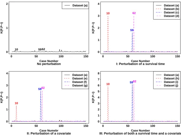
We selected cases 10, 59 and 62 for perturbation. To create influential observations in the dataset, we choose one or two of those selected cases and perturbed the survival time (yi), the covariate (xi1), or both the survival time and the covariate of the chosen
case(s). For the above perturbations, the survival time for theith case was perturbed as ˜yi = yi + 5ˆσy, where ˆσy is the standard deviation of the yi’s. And the covariate x1
for theith case was perturbed as ˜xi1 =xi1−5ˆσx1, where ˆσx1 is the standard deviation
of the xi1’s. After perturbing the survival time, the survival time of cases 10, 59, and
62 were changed from 0.01820 to 0.67849, 0.06854 to 0.72883, and 0.06765 to 0.72795, respectively. After perturbingx1, the value of this covariate for cases 10, 59 and 62 was
then changed from -1.39632 to -6.39632, -0.60912 to -5.60912, and -1.31305 to -6.31305, respectively. Specifically, we considered 6 different types of perturbation schemes: (I) perturbation of a survival time for a case; (II) perturbation of a covariate for a case; (III) perturbation of both a survival time and a covariate for a case; (IV) perturbation of a survival time for two cases; (V) perturbation of a covariate for two cases; (VI) perturbation of a survival time for one case and a covariate for another case. Detailed descriptions regarding the perturbations are given in Table 2.1. In Table 2.1, dataset (a) denotes the original simulated dataset with no perturbation and datasets (b)-(o) denote datasets with perturbed case(s) added by the perturbation schemes (I)-(VI).
We fit the gamma process model of Section 2.3 with an exponential H∗(y) = 2.7y. We chose a noninformative prior distribution for β as N2(0,106I). We used ARMS
within Gibbs to obtain posterior samples. After burn-in, 40,000 MCMC posterior sam-ples were used in the analysis. The proposed joint and marginal K-L divergences, K(P, P−i) in (2.10), K(P1, P1,−i), K(P2, P2,−i) in (2.16), and calibrations of those
andK(P2, P2,−i). We monitored convergence of the Gibbs chain using the method
pro-posed by Geweke (1992), as well as trace plots. We conducted sensitivity analyses using c=0.01, 0.1, 1, 10 and 100. For brevity, we present results for only the low confidence value of c=0.01. For the computation of K(P1, P1,−i) and K(P2, P2,−i), we used every
5th sample from the 40,000 MCMC posterior samples to reduce the autocorrelations and yield better convergence results.
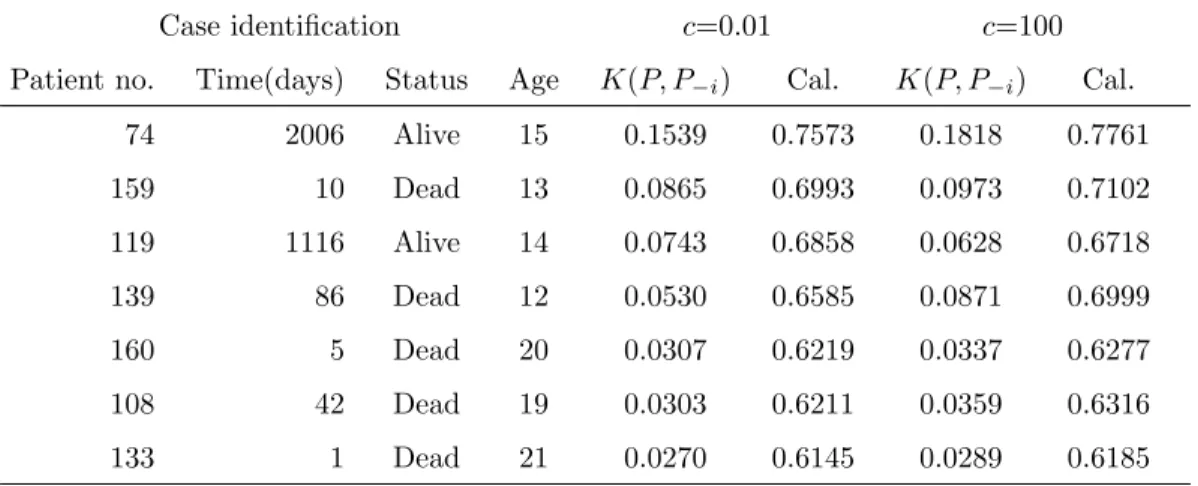
Table 2.1 shows that the posterior inferences are sensitive to the perturbation of the selected case(s). Overall, the inferences are most sensitive to the perturbation of both the survival time and the covariate. Since we used noninformative priors onβand c=0.01, the posterior estimates were similar to the maximum likelihood estimates based on partial likelihood. The results regarding the diagnostics showed that K(P, P−i), as
well as K(P1, P1,−i) and K(P2, P2,−i), changed very little for the non-perturbed cases,
while they changed a lot for the perturbed case(s).
The results in Table 2.2 show that before perturbation (dataset (a)), all of the selected cases are not influential, each providing a small K(P, P−i) with its calibration
close to 0.5. However, after perturbation (datasets (b) through (o)),K(P, P−i) for those
perturbed cases increased a lot and the corresponding calibrations become much larger than 0.5, indicating those cases are influential. Specifically, perturbing both the survival time and the covariate of a case increasesK(P, P−i) a lot. For example,K(P, P−i) (and
its calibration) for case 10 in dataset (h) is increased from 0.0006 (0.5168) to 5.8040 (1). We also note that the perturbed cases are similarly identified as influential using the likelihood displacement (LD) based on partial likelihood. Moreover, Figure 2.1 clearly shows that K(P, P−i) performed well for identifying influential case(s) in each dataset
providing larger K(P, P−i) for the perturbed case(s) compared to the other cases.
Moreover, in Table 2.1, we observe that perturbing the survival time of a case had influence on the posterior estimates of both β1 and β2, while perturbing the