Mace_thesis_final.pdf

(1)

Simulating the Thermal Evolution of Dark

Matter During an Early Matter-Dominated Era

By Charlie Mace

Senior Honors Thesis

Department of Physics and Astronomy University of North Carolina at Chapel Hill

May 1st_{, 2020}

Approved:

Dr. Adrienne Erickcek, Thesis Advisor

Dr. Lu-Chang Qin, Reader

(2)

Acknowledgements

(3)

Abstract

The period between inflation and the onset of Big Bang nucleosynthesis is, in many ways, poorly understood and poorly constrained. In particular, the ramifications of including an early

matter-dominated era (EMDE) in this period have not been fully explored. One possible probe of this era is the evolution of dark matter. The precise way in which WIMP dark matter

decouples from the relativistic bath has a profound effect on the smallest scale (kcut) of structure

formation, which then influences annihilation signatures that can be observed by Fermi-LAT. There has already been work connecting kcut to the annihilation signatures, but there is a missing

link between fundamental particle physics and kcut itself. The goal of this work is to begin to

close that gap, by connecting dark matter microphysics to kcut. The thermal evolution of dark

matter during radiation domination can be solved analytically, but the inclusion of an EMDE violates key assumptions made in the analytical solution. To understand the effect of an EMDE on the velocity distribution of dark matter, we model the collisions between individual dark matter particles and relativistic leptons. In this work, we use UNC’s Longleaf Cluster to evolve an ensemble of 15,000 dark matter particles through both the EMDE and the subsequent transition to radiation domination. We find that the shape of the velocity distribution deviates significantly from the analytical solution and that the new distribution is not well described by the dark matter temperature. This represents a breakdown of the analytical solution for the momentum distribution when decoupling deep in an EMDE, making this numerical simulation necessary in order to calculate kcut and connect a particular dark matter candidate to observable

(4)

1. Introduction

1.1. Motivation and Outline

While much of the Universe’s history is well constrained, there is a significant gap in our knowledge during the first second after inflation. Observational astronomy cannot see beyond recombination because the Universe is opaque at earlier times, and constraints from the relative abundances of light nuclei can only tell us about the state of the Universe at the end of this one second gap. In particular, this gap is typically assumed to be dominated by radiation, but may very well be dominated by something that behaves like matter. We refer to this scenario as an early matter-dominated era (EMDE). If dark matter is weakly interacting, its interactions with leptons in this time may give some clue of what is happening in this era, and whether or not an EMDE exists.

The dark matter - lepton interactions are well understood in the typical case of radiation domination, but including an EMDE invalidates some key assumptions that led to this

understanding. In this work, we develop a simulation that models individual collisions between dark matter and leptons. This more fundamental approach avoids the assumptions used in the radiation dominated case which are now faulty, and shows us how inclusion of an EMDE changes the evolution of dark matter.

Section 1 lays the groundwork for this thesis, giving an introduction to the principles and

terminology of cosmology required to understand the questions being asked. Section 2 uses these principles to approach the dark matter - lepton interactions happening in the era of question, and explores the failure of the traditional approach in the case of an EMDE. Section 3 outlines our approach to solving this problem. This includes an outline of the simulation, as well as the calculation of all the parameters needed to execute the simulation and interpret the results. Section 4 give the results of our simulation, and section 5 assesses these results and outlines plans for future work.

1.2. An Expanding Universe

One of the fundamental facts of cosmology is that the Universe is expanding; two points in space move further apart over time. This concept can be quantified by defining two different types of distances: physical distance and comoving distance, denoteddand xrespectively. The comoving distance is thought of as the distance on some grid that expands along with space. As space expands, the grid expands as well. The comoving distance between two objects remains the same, and we can consider objects as being stuck to this grid (barring any motion that is not attributable to cosmic expansion). The physical distance refers to the actual distance between two points as we could measure, which is increasing over time. These two distances are related by the scale factor, denoted a, asd=ax. The scale factor is a dimensionless value that quantifies cosmic expansion. The actual value of ais not meaningful; all that matters is the change ina over time. For example, if at time t1 a1= 1, and at timet2 a2= 3, then the physical distances separating objects has increased three-fold. The exact same would be true if we saida1= 2 and a2= 6,a2= 3a1, so space has expanded by a factor of three. The point in time wherea= 1 is defined is totally arbitrary, and is chosen to be whatever is convenient for the work being done.

(6)

H≡ da

dt

1

a. (1.1)

IfH is very large the Universe is expanding quickly, and if H is very small it is expanding slowly. IfH were negative, then the Universe would not expanding, but shrinking. This expansion rate is directly tied to the contents of the Universe, as dictated by the first Friedmann equation:

H2= 8π 3m2

pl

ρtotal, (1.2)

wherempl is the Planck mass (a constant), andρtotal is the total energy density of the Universe.

The actual evolution ofρtotal can be quite complicated, since it accounts for all types of energy in

the Universe, each of which can have a different relationship witha. In practice, nearly all of the Universe’s history can be well understood by identifying what species of energy constitutes the majority of the Universe at a given time, and neglecting the rest in the calculation of H. We say that the species constituting the vast majority of the Universe’s energy density dominates the Universe, and studying these distinct eras can give a remarkably complete understanding of the Universe’s history. The transition between the eras must be treated with more care, but physics deep within an era can be greatly simplified by neglecting the non-dominant species.

To understand these eras, we must analyze each major component of the Universe, relating its energy density to the scale factor. We will begin with matter, as it is relatively straightforward. ConsiderN particles, each of mass m, in a box with sides of length d. Assuming the particles are evenly distributed, the mass density is given by by the total mass divided by the physical

volume, ρm=mN/d3=ρm=mN/(ax)3∝a−3. The number of particles in the box stays the same,

since the particles are stuck to the comoving grid, but the physical volume of the box has

increased. As the Universe expands, the amount of matter in each comoving box stays the same, but the amount in a physical box is proportional toa−3_{. Therefore, matter density scales as} _a−3_.

Next we consider radiation, by which we mean any relativistic particle. We will explicitly consider a photon, and by the end of this section we will see that this solution applies to all relativistic particles. By the same argument as above, the expanding physical volume of the Universe will contribute a factor of a−3 to the scaling of the radiation energy density ρr. In this

case however, the energy contained in a comoving box will not be constant. In the matter

example, the massm of each particle was invariant as space expands. In the case of a photon, we need to consider the relation between wavelength and energy. A photon with wavelengthλhas an energyE= hc_λ, wherehis Planck’s constant, and c is the speed of light. Sincehand c are constant, we haveE∝λ−1_{. As space expands, the physical separation between peaks of a wave} increases, which increases the wavelength, an effect called cosmological redshift. Since λis a physical distance, we have λ∝a, giving E∝a−1_{. From this argument we see that in addition to} the physical volume of a comoving box increasing asa3_{, the energy contained in that box is also} decreasing asa−1_{. Since the energy density is defined as the energy per physical volume, we can} combine these factors and find thatρr∝a−4.

The evolution of a generic species of energy can be understood by introducing the second Friedmann equation:

d2a

dt2

1

a=−

4π

3m2

pl

(7)

where we have introducedP as the total pressure of the Universe. By combining the two Friedmann equations, we get:

dρ

dt + 3H(ρ+P) = 0. (1.4)

This represents the conservation of energy in general relativity. Energy can be exchanged

between the local energy density ρand the spacetime geometry, and that exchange is governed by the rate of expansionH. IfH = 0, there is no expansion, and energy conservation takes the well-known form of d_dρ_t = 0. To get the evolution of ρfrom this equation, we must characterize the relationship between energy and pressure. This relationship is given by the equation of state parameter, denoted w, asP =wρ. Plugging this into equation (1.4), we get:

dρ

dt + 3(1 +w)Hρ= 0. (1.5)

Changing from a time derivative to a scale factor derivative allows this equation to be quickly solved, finding:

ρ∝a−3(1+w). (1.6)

Matter is pressureless, so w= 0. Equation (1.6) then gives ρm∝a−3, as we argued previously.

Similarly, w= 1/3 for radiation, givingρr∝a−4.

The final piece of information we need before moving forward is how momentum evolves in an expanding spacetime. As any particle travels through spacetime unperturbed, the evolution of its four-momentum is governed by the geodesic equation. In the case of expanding spacetime, this results in a redshifting of momentum,p∝a−1_{. This effect is referred to as Hubble friction, as it} has the result of particles “sticking” to the comoving grid, with any peculiar velocity dissipating as the Universe expands. This momentum evolution generalizes the arguments for ρr∝a−4

above. The energy and momentum of a relativistic particle are approximately equal, so the energy density picks up an additional factor of a−1 _{leading to} _a−4 _{scaling, just as we saw with} photons.

1.3. A Brief History of the Universe

Armed with our understanding of energy density evolution, we can categorize the history of the Universe into four major eras (see figure (1)). This will inform the growth of structure

-inhomogeneities in the distribution of dark matter - that eventually lead to the formation of the stars, galaxies, and clusters that we see today. The first era is inflation; a period of accelerating expansion, proposed in order to correct for the flatness and horizon problems in cosmology [2]. The dominant form of energy in the Universe during inflation is a scalar field called the inflaton [3], which is destined to eventually decay into other forms of energy.

(8)

Figure 1: The four major eras of the universe: inflation, radiation domination, matter domination, and dark energy domination [1].

nucleosynthesis (BBN), and recombination. BBN occurs at a temperature on the order of 0.1 MeV, when neutrons and protons form stable nuclei (primarily helium). This process establishes the relative abundances of light nuclei in the Universe, allowing measurements of these

abundances today to provide a detailed look into the state of the Universe at this time. Once the radiation has cooled even further, to a temperature on the order of 0.1 eV, free electrons can be bound to free protons without being immediately ionized by the radiation bath, forming neutral hydrogen. This is called recombination, and marks the earliest time that the Universe is

transparent to photons [1].

As the Universe expands, radiation energy density decreases faster than matter disperses, eventually causingρr to drop below ρm, leading to a matter dominated era. Once matter is the

dominant form of energy, it begins to form structure as matter is drawn to gravitational potential wells, forming larger structure that will lead to galaxies and clusters [1].

After matter domination comes dark energy domination, the current era. This change occurs when, much like the shift from radiation domination to matter domination, the energy density of matter falls below the density of some other energy, dubbed dark energy. The exact nature of the dark energy dominating the Universe is unknown, but this era is characterized by the empirically determined accelerating expansion of the Universe [5]. Whatever the source of dark energy, the accelerating expansion suppresses the formation of larger structure [1]. This means whatever structure we see today was likely formed long ago, during earlier eras.

1.4. The Case for an Early Matter Dominated Era

(9)

growth. The Universe before recombination is opaque to light, but detailed information about its state at the time of BBN can be inferred from observations of the relative abundances of

hydrogen, helium, and other light nuclei. Prior to BBN, however, is much more difficult to constrain. Some theories of inflation promise inflationary gravitational waves that could carry information about the earliest moments of the Universe, but at the moment these are out of reach of current gravitational wave detectors [6]. This leaves a large unconstrained era in the Universe’s history: between the end of inflation and BBN. Planck gives an upper bound on the energy scale of inflation on the order of1016 _{GeV [7], and BBN occurred at the MeV scale. If the} entire period were radiation dominated, the Universe expanded by a factor of1019 between inflation and BBN. In the standard model of the Universe described above, this period is

considered to be radiation dominated. This is simply chosen because it is the simplest model. We know that BBN must occur during radiation domination, so why add another era between

inflation and radiation domination without evidence? There are, however, many theories which would suggest an early matter-dominated era (EMDE) between inflation and BBN.

One model that produces an EMDE is the case of a long-lived inflaton. Inflation ends when the inflaton begins oscillation around the minimum of its potential before decaying. If this oscillation is in a quadratic potential (which becomes a valid approximation for very small oscillations, even if the potential is not quadratic globally), the inflaton evolves as a pressureless (w=0) fluid does. This produces the same energy scaling as matter, so while the oscillating inflaton dominates, the Universe is in an effective matter dominated era [8]. In this scenario, dark matter itself is not the dominant energy density, but rather the oscillating inflaton which behaves like another species of matter.

The second case is motivated by string theory. String theory predicts many gravitationally coupled heavy scalar fields [9], producing them as dimensions are folded up via compactification. Any or all of these scalar fields could come to dominate the Universe, before decaying away. Similar to the inflaton case, this oscillation could produce an EMDE. The string theory

proposition for an EMDE leads to other complications however. The abundance of scalar fields can interfere with the tightly constrained BBN, leading to the Cosmological Moduli Problem [9].

(10)

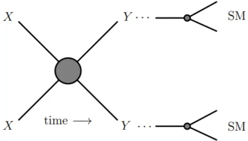
Figure 2: A diagram of hidden sector interactions. The stableX annihilates into the unstable Y, which then couples to the Standard Model. Once X annihilations are rare, it is effectively decoupled from the Standard Model [11].

Figure 3: Left: A subhorizon perturbation. Since k−1 _< ₍_aH₎−1_{, the perturbation can grow.} Right: A superhorizon perturbation. In this case, k−1 > (aH)−1, and the power of the modek is frozen until the horizon expands and it re-enters.

extension, from the visible sector.

Now that we have changed the timeline of the Universe, we need to slightly adjust our terminology. Previously, reheating referred to the end of inflation and beginning of radiation domination. Now that we have inserted an era between these two events, we need to decide which reheating corresponds to. When discussing an EMDE, reheating refers to the decay of the dominant energy species into radiation. This marks the end of the EMDE, not the end of inflation.

1.5. Structure Growth

(11)

understand how such perturbations evolve.

Analyzing structure as a function of space, constructing a function that describes over-dense and under-dense regions, is possible. It is much easier, however, to analyze inhomogeneity in Fourier space. The distribution of matter in space can be expressed as an infinite sum of periodic functions, each with a different comoving wavenumberk. These wavenumbers are the spatial frequency of the oscillation; a large kis a very small scale perturbation, and a smaller k is a larger scale perturbation. Since each perturbation of scalek will evolve independently from perturbations of other scales [1], we can study them individually, greatly simplifying the work.

To get a frame of reference for the size of the mode, we can compare it to thecomoving horizon

(aH)−1. This is approximately the size of the observable Universe; it is the farthest apart that two causally connected points can be. If the distance separating two objects is larger than the comoving horizon, they are not causally connected and cannot communicate. We can consider two cases fork: k−1(aH)−1 and k−1(aH)−1. If the former is true, then the scale of the perturbation is much larger than the size of the Universe, and we say that the mode is superhorizon. In the latter case, then the reverse is true, and we say the mode is subhorizon. Both cases can be seen in figure (3). The comoving horizon is plotted in figure (4), and here we see that many modes exit the horizon during inflation and re-enter it afterwards. Since the peaks of superhorizon modes are outside of the observable Universe and thus causually disconnected, we find thatperturbation growth is frozen for superhorizon modes. In contrast, subhorizon modes grow with time, as the gravitational potential draws in more matter. An example of a mode entering the horizon and beginning growth is shown in figure (5).

We can more quantitatively understand the growth of structure by introducing thepower spectrum P(k, a), which is the Fourier transform of the matter density. The primordial power spectrum is seeded by quantum fluctuations in the very early Universe, but after this point not all perturbations evolve equally. Through the evolution of the Universe different scales are suppressed and boosted through various mechanisms. The rate at which perturbations grow depends on the dominant species of energy. During matter domination P ∝a, and during

radiation dominationP ∝ln(a)[1]. This means growth is faster in matter domination, and slower in radiation domination.

Since modes are frozen until they enter the horizon, this adds another layer of complexity onto the power spectrum. While all subhorizon modes grow at the same rate at any given time, modes that enter earlier have a head-start, and will be boosted in the power spectrum. Thisk

dependence is given by the transfer function T(k), which contains thek dependence ofP(k, a). The transfer function will also account for the random thermal motions of dark matter particles, referred to as free streaming, which washes out small-scale structure. This creates a maximum valuekcut that gives the smallest scale where free streaming doesnot prevent structure

formation. This free streaming cutoff is discussed more quantitatively in the following section.

1.6. Connecting Annihilation Signatures to the Early Universe

(12)

Figure 4: The comoving horizon(aH)−1_{, compared to a comoving length scale}_k−1_{. The mode} k exits the horizon during inflation atak, and its power is frozen. During radiation

domination the comoving horizon becomes large enough fork to re-enter, become a subhorizon perturbation again. After this point it can resume growth. Ifk were larger, corresponding to a smaller scale perturbation and smaller k−1_{, then this mode would} have re-entered the horizon earlier, and had a longer growth period. Figure adapted from [16].

Figure 5: The growth of a single perturbation through an EMDE. δdm is the fractional

overdensity(ρdm −ρdm)/ρdm, and the perturbation here is normalized to the initial

(13)

discussed previously, an annihilation process is expected to exist. These annihilation signatures will be coming from dark matter halos, overdense regions of dark matter where interactions are more likely. Halos that form in the early Universe form in a higher density environment, making the halos themselves denser. The annihilation rate scales with density squared (it takes two particles to annihilate), so denser halos have stronger annihilation signatures [17, 18].

Next we need to understand the connection between when these halos form, and how much stronger the annihilation signature is. The boost factor to the annihilation rate B= Γ/Γ0 (where

Γ is the annihilation rate with microhalos andΓ0 is the annihilation rate without microhalos) is proportional to the dark matter density at the redshift of structure formationzf, which is

proportional to(1 +zf)3, since redshift and the scale factor are related bya= (1 +z)−1. The

boost factor is also proportional tof(zf), where f(zf)is the fraction of dark matter bound in

halos at zf. A small change inzf has a major effect on B, and B must be understood before

interpreting observed annihilation rates. The effect of kcut on the bound dark matter fraction

(through a changingzf) can be seen in figure (6). This then causes a boosted annihilation

signature.

To predict the redshift of formationzf, we need to understand the power spectrum. In particular

we need to understand the effect of an EMDE on the free streaming cutoff kcut. In cosmological

models without an EMDE, the value of kcut has little effect on when microhalos form. This is

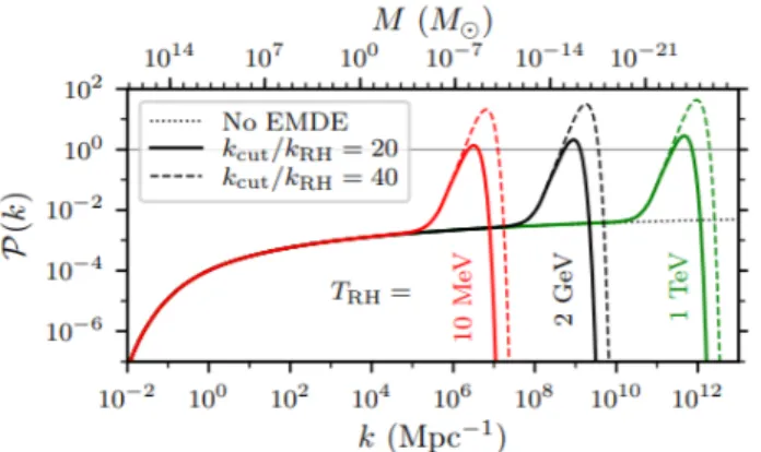
because the power spectrum is nearly flat for largek (as seen in figure (7)), since they all entered the horizon during radiation domination when perturbations only experience logarithmic growth. In an EMDE however, kcut is crucial to the understanding of microhalo formation. The modes

that are within the horizon during the EMDE get a large boost as they experience linear growth, while the larger scale perturbations are frozen outside. This sharply boosts the power spectrum on small scales. This boosted part of the power spectrum reaches the threshold for structure formation before the lower portions, allowing microhalos to form before other structure formation occurs [18]. Now the importance of kcut is clear; since the power spectrum is linear on the

boosted end, a small change in kcut significantly alters the redshiftzf where formation begins.

To predict kcut, we need to understand how the dark matter momentum distribution function

evolves during an EMDE. This is because the momentum distribution gives us the thermal velocities, which determines how much structure can be wiped out by free streaming [17]. A higher dark matter velocity means there is more free-streaming, hindering the formation of small-scale structure. This suppression of small-scale structure gives uskcut, above which there is

no structure formation [15].

The effect ofkcut on the power spectrum enhancement is very strong, as seen in figure (7). This

translates to a very delicate relationship between kcut and the bounds annihilation signatures

places on dark matter candidates. Figure (8) shows that a factor of two difference in kcut

significantly changes how much dark matter parameter space is ruled out by Fermi-LAT observations of microhalo annihilation signatures. This tight relationship between the dark matter parameter space and the cutoff scale means thatkcut must be known very precisely if we

are to confidently translate it to bounds on dark matter candidates and the evolution of the early Universe.

(14)

Figure 6: The effect ofkcut on the bound fraction of dark matter in small halos. A larger value of

kcut leads to more bound dark matter, because structure formation begins at an earlier

zf [18].

parameter. In order to predict this final momentum distribution, we must understand the interaction between the dark matter population and the leptons during an EMDE. This interaction is the topic of the next section.

2. Understanding Decoupling

As seen above, the evolution of the dark matter velocity distribution is essential in the

connection between dark matter physics and observable annihilation signatures. To understand this evolution, we must understand how it interacts with the relativistic lepton bath in the early Universe. At early times when the Universe was very dense, weak interactions between WIMPs and the relativistic lepton bath were frequent. This constant scattering allowed a free transfer of momentum between the two populations, causing them to thermalize to the same temperature. At later times these interactions became rarer, and eventually nonexistent, as the space between the leptons and the WIMPs expanded faster than these scatterings could happen. Once there are no scatterings, we expect the temperatures of the radiation and the WIMPs to diverge, following the expected evolution for radiation and massive particles respectively. We say at this point that the two populations have decoupled. To predict the final temperature - and thus the final

(15)

Figure 7: The power spectrum for various values ofkcut and TRH, the temperature of reheating.

The value ofkcut is where the transfer function sharply drops, and kRH is the wave

entering the horizon at reheating. The upwards bump is the enhancement in the power spectrum due to an EMDE, where scales in the boosted range are inside the horizon and thus grow linearly. We see that for everyTRH, a factor of 2 change in kcut increases

the size of the enhancement by roughly an order of magnitude. In contrast to the EMDE cases, the scenario where there is no EMDE produces a flat power spectrum [19].

Figure 8: The effect ofkcut on the dark matter parameter space for two different TRH values:

10 MeV (left) and 2 GeV (right). The y-axis is the annihilation cross section, and thex-axis is the dark matter mass. The red region on the left is the requirement that the Universe is not closed, and the grey region on the right is where the dark matter coupling constant exceeds unity. The green and blue regions are the Fermi-LAT bounds forkcut/kRH of 20 and 40 respectively. In order to get the observed dark matter relic

(16)

2.1. The Standard Approach to Dark Matter Temperature Evolution

An analytical solution can be found in the case where the typical momentum transferred in a collision is very small relative to the total momentum of the dark matter particle. This scenario can be understood with the analogy of a bowling ball (the dark matter particle) moving through a sea of feathers (the leptons). While each individual collision has little effect on the bowling ball, the influence of many collisions add up, and appreciably change the bowling ball’s motion.

The typical momentum transferred in a dark matter - lepton collision in this scenario will be on the order of the lepton momentum kSince the leptons are relativistic we have that the lepton momentum is approximately the lepton temperature TL for a typical lepton. The typical

momentum pof a dark matter particle can be found from the definition of temperature: Tχ≡ 2₃hKEi=2₃hp

2_i

2mχ, giving a typical momentum ofp'

p

3mχTχ. We now have ∆p/p'TL/

p

3mχTχ. If we consider a very massive dark matter species, it may seem

straightforward to convince ourselves that the conditionmχ TL is sufficient to ensure∆p/p1,

but this is not quite the case. In reality, the required condition is exactly what we solved for, namely thatTL

p

3mχTχ, which we will refer to as the Boltzmann approximation. It turns out

that while the Boltzmann approximation does not hold in general, in radiation domination (which is the standard scenario), it only breaks down after collisions have stopped significantly affecting the dark matter momentum. TL and Tχ are approximately equal prior to decoupling,

and while Tχ eventually cools to the point where this approximation breaks, by the time this

happens collisions are negligible.

To see this, we have to introduce three quantities: the Hubble expansion rateH, the momentum transfer rateγ, and the collision rateΓ. γ is the rate at which momentum is transferred between the relativistic bath and the dark matter population, andΓ is the rate at which collisions occur. The ratio γ/H is most easily understood by writing it as (1/H)/(1/γ). We interpret1/γ, which has units of time, as the typical time taken to transfer an amount of momentum appreciable to the dark matter momentum, i.e. the amount of time for collisions to significantly affect the dark matter particle. 1/H is approximately the age of the Universe, which means our fraction

(1/H)/(1/γ)is indicative of whether or not collisions have a meaningful impact on the dark matter momentum once we consider the redshift ofpχ caused by the expanding Universe. If 1/H 1/γ, then the age of the Universe is much longer than it takes for collisions to significantly affect the dark matter momentum on small timescales, so there is a significant transfer of

momentum between the populations. If 1/H1/γ, then the time taken to transfer momentum is much longer than the age of the Universe, and the effect of collisions onpχ is overpowered by the

redshifting due to the expansion of the Universe. Through similar reasoning,Γ/H is the comparison between the time between collisions and the age of the Universe. IfΓ/H1, then collisions happen very frequently. If Γ/H1, then collisions are rare.

If we take the Boltzmann approximation to be valid, we can obtain an analytical solution to the dark matter temperature evolution. Before any approximation, the evolution of the dark matter distribution function is described by the Boltzmann equation [1]:

df

dt =C[f], (2.1)

(17)

and the total derivative of f is 0. This means that the number of particles within a given volume inphase space, a six-dimensional space that includes a particle’s momentum in addition to physical location, is constant. The complication arises when we considering expanding and otherwise changing spacetime. Expanding the total derivative gives:

df

dt = ∂f

∂t + ∂f ∂x

dx

dt + ∂f ∂p

dp

dt. (2.2)

While the number of particles in a phase space element may be constant, that element itself can change through time. In a homogeneous and isotropic Universe, the only effect of this

consideration is the final term of equation 2.2. This accounts for the fact that momentum redshifts asa−1_.

The next complication is inC itself. The effect of collisions is accounted for with the Boltzmann collision integral. This integral is given in full in equation 3.6, and discussed in greater deal there. For our current purposes, it is sufficient to recognize that if the Boltzmann approximation is made, then the Boltzmann equation can be simplified as shown in [20], producing a new form of the collision term:

_df 0 dt

c

=γh3f0+

*

p·*∇pf0+mχTL∇2pf0 i

. (2.3)

Here we recall that γ is the momentum transfer rate, giving the rate at which momentum

transfers between the lepton and dark matter populations, and we now have f0 as the momentum distribution function in the absence of perturbations. The matrix element|M|2_{, which gives the} scattering amplitude and hence the scattering likelihood, is proportional to γ [20]. This is the term of the Boltzmann equation that accounts for momentum change due to collisions, hence the subscriptc. As detailed in [20] and appendix A, these simplifications show that a

Maxwell-Boltzmann distribution is a solution to this equation. Once the dark matter has decoupled from the leptons, the momentum distribution maintains its shape as it redshifts away asa−1, meaning our dark matter population should be eternally Maxwell-Boltzmann. The temperature of this distribution is found to obey the differential equation:

adTχ

da + 2Tχ=−2 γ

H(Tχ−TL). (2.4)

Explicitly considering radiation domination, we can make some quantitative observations from equation (2.4). Whileγ/H 1, the right side of the equation dominates the evolution of Tχ,

forcingTχ'TL. This is consistent with the intuition developed above: the collisions are

imparting a significant amount of momentum, the two populations thermalize, and the dark matter temperature is bound to the lepton temperature. In the limit ofγ/H 1 it is often assumed that the right side of equation (2.4) is negligible. It is clear that the (γ/H)Tχ term is

much less than the left side in this case, but the reasoning behind discarding the(γ/H)TL term is

less obvious. In radiation domination, we haveH ∝T2_∝_a−2_{. This gives}₍_γ/H₎_T _∝_a−5_{, once we} use the typical case whereγ∝T_L6 [20]. The homogeneous solution to the differential solution givesTχ∝a−2, so thea−5 scaling quickly makes the contribution of this term negligible. We are

therefore safe in neglecting the right side. Considering the left side to be dominant, we can take the homogeneous solutionTχ∝a−2 when γ/H 1. As our intuition suggested, this is simply the

(18)

10-7 10-6 10-5 10-4 10-3 10-2 10-1 100 101 102 103

100 101 102 103 104 105 106 107 108 109

Temperature (GeV)

scale factor (a) T ~ T a-3/8

= H

Quasi-Decoupled

T a-9/8

Reheating T a-1

T a-2 T

T

Figure 9: The quasi-decoupling solution for dark matter temperature evolution. Whenγ/H = 1, Tχ diverges from the lepton temperature, but it does not fully decouple until reheating

[17].

2.2. Decoupling in an EMDE

The analysis of decoupling given above changes significantly when considering an EMDE. The source of the EMDE (whether an oscillating scalar field or hidden sector particle) is decaying into radiation, which injects entropy into the relativistic bath and causes the radiation energy density to scale asρR∝a−3/2 rather than the typicalρR∝a−4. This entropy injection supports the

lepton temperature, causingTL∝a−3/8 [21, 22].

To understand the evolution ofTχ in an EMDE, we have to revisit equation (2.4). The case

whereγ/H 1 still forces the right side to dominate, tightly couplingTL and Tχ as expected.

The γ/H1case, however, is not as simple as before. In an EMDE, TL is supported by the

entropy injection from the decaying scalar field. In addition, our dominant energy density evolves as matter, which givesH ∝√ρm∝a−3/2 (equation 1.2)). This causes(γ/H)TL∝TL3∝a−9/8. This,

unlike thea−5 _{scaling in the radiation dominated case, is not steeper than the homogeneous} solution, so this term can not be neglected as easily. Including this term we can solve for the new Tχ evolution, and findTχ∝a−9/8. This is faster than the tightly coupled a−3/8 scaling, but slower

than thea−2 _{scaling seen when fully decoupled in radiation domination. This represents an} intermediate stage in dark matter decoupling between the fully coupled and totally decoupled state, which we call quasi-decoupled [17, 21]. TheTL and Tχ evolution we argued above can be

seen when solving equation (2.4) numerically, and is shown in figure (9).

There is a major issue with the above analysis. If the solution to equation (2.4) is to be believed, then the dark matter is quasi-decoupled for the entire period between kinetic decoupling and reheating. There are, however, scenarios where this result is nonsensical. We consider a dark matter candidate that kinetically decouples well before reheating if we choose the kinetic decoupling temperatureTkd to be much larger thanTRH. After kinetic decoupling, specifically

(19)

away withp∝a−1 _and _T

χ∝a−2. If this occurs before reheating however, our above solution

predicts quasi-decoupling, andTχ ∝a−9/8. Since there are no collisions occurring, this result is

clearly impossible. In fact, equation (2.4) does not includeΓ/H at all, meaning that whether or not collisions are actually occurring plays no role in this prescription for kinetic decoupling. This indicates that our analytical solution is no longer valid.

The source of the error is the Boltzmann approximation, which was used to derive the collision operator in equation (2.3). While we previously argued that the approximation held as long as collisions were significantly affecting the dark matter momentum, this argument was for radiation domination. In an EMDE, due to the comparatively shallow γ/H∝a−4/3 _{evolution, collisions are} relevant beyond the range of validity of the Boltzmann approximation. The invalidity of the Boltzmann approximation while collisions still affect the evolution of the dark matter momentum means that the collision operator in equation (2.3) is no longer valid, so we have no reason to believe that the differential equation derived from it accurately describes the evolution ofTχ.

Furthermore, the expectation that the dark matter momenta follow a Maxwell-Boltzmann distribution with temperature Tχ followed from this derivation [20], so the distribution function

may deviate significantly from Maxwell-Boltzmann. Since no analytical solution is available, we must turn to more fundamental physics for a solution.

3. Monte Carlo Simulation

To solve the problem without relying on the Boltzmann approximation made in deriving equation (2.4), we will return to the initial form of the Boltzmann collision integral and simulate the evolution of dark matter particles by calculating the outcomes of individual dark matter - lepton collisions. This will be done for relativistic leptons (kmL) and non-relativistic dark matter

(pmχ), but without the faulty assumption thatTLp3mχTχ.

3.1. Outline of Procedure

The below process will be performed for a single dark matter particle, simulating the Weak collisions between that particle and the relativistic lepton bath. This assumes the dark matter is not self interacting, or that self interactions are negligible compared to the lepton interaction. We also assume that the dominant species of the EMDE (which will hereafter be referred to as the scalar field for ease, although there were other possibilities discussed in 1.4) is only transferring energy into radiation; our dark matter population is sourced from pair production well before reheating, and is not gaining or losing particles.

The simulation runs from a very early time (largeγ/H) whereTL'Tχ, and ends after reheating,

when the dark matter and leptons are totally decoupled and no collisions are occurring. To get the initial dark matter momentum p, we use use a Metropolis Hastings algorithm [23], which is a Monte Carlo Markov Chain (MCMC) method to sample distribution functions. This method samples from a Maxwell Boltzmann distribution atT =Tχ=TL. The details of the Metropolis

Hastings MCMC algorithm will be discussed in section 3.5.

Once the initial momentum has been sampled, the simulation proceeds in a series of timesteps, stopping once the endpoint has been reached. In each timestep, the following steps take place:

(20)

the timestep. Generate a random numberQ∈[0,1]; ifQ < P, then a collision occurs. Otherwise, no collision occurs, and the algorithm skips to the redshift (step #4).

2. Sample collision parameters: Once it has been determined that a collision is occurring, there are four free parameters of that collision that must be chosen in order to fully

determine the final momenta. These parameters are:

a) The initial lepton momentum*k, which can be described by its i. magnitudek

ii. angleθi with respect to the initial dark matter momentump.

b) The scattering angles in the center of momentum (COM) frame

i. θCM, with respect to the line of collision formed by the initial dark matter and

lepton momenta in the COM frame

ii. ϕCM, with respect to the collision plane formed by the initial dark matter and

lepton momenta in the comoving frame

3. Calculate the outcome of the collision: Once we have all the collision parameters, we can calculate the new dark matter momentum, and update paccordingly.

4. Apply redshift: Once the possible collision has been taken care of, we must calculate how much the dark matter redshifts due to the expansion of the Universe. This is simple, as momentum always redshifts asa−1_.

Now that we have laid out the structure of the simulation, we have a list of things that must be calculated before we can proceed. First we need the evolution of both the background parameters (such asH and TL) and the collision rateΓ. TheTL and H evolution is shown in 3.2, and

sections 3.3, and 3.4 lead to Γ. Next we need to sample for the collision parameters. This will involve the calculation of the non-trivial Boltzmann collision integral, and the implementation of a multi-dimensional Metropolis Hastings algorithm. These are done in sections 3.3 and 3.5 respectively. Finally, the relativistic kinematics for the collision must be calculated. This is lengthy, and is done in appendix C.

3.2. Background Evolution

We are considering the scenario of a scalar field decaying into only radiation. DefiningTRH to be

the temperature at which the scalar decay rateΓϕ is equal to the Hubble expansion rate, we find:

Γϕ=H(TRH) =

r

8π2_g

∗(TRH)

90

T_RH2 mpl

(3.1)

whereg∗ is the number of relativistic degrees of freedom, andmpl is the Planck mass. With this

decay rate, we can write the coupled differential equations describing the evolution of the scalar field and radiation energy densities:

d

dtρϕ=−3Hρϕ−Γϕρϕ

d

dtρr=−4Hρr+ Γϕρϕ.

(3.2)

(21)

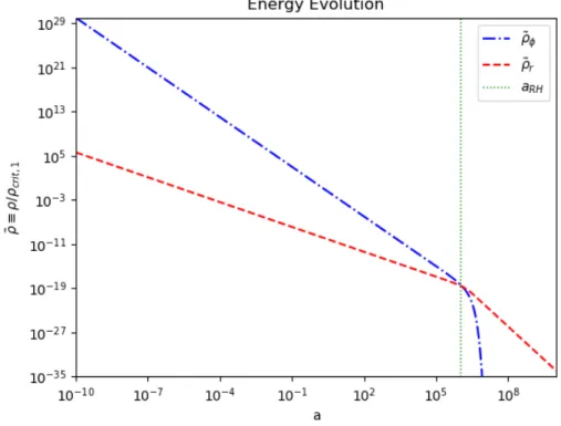
Figure 10: Numerical solution for the coupled energy density equations in equation 3.2. This solution is forTRH = 0.01MeV and aRH = 106, the parameters used in the MCMC.

the scalar field to the radiation bath; it is positive in the radiation equation because energy is being added to the radiation, and negative in the scalar field equation because energy is being lost from the scalar field. H can be related to the energy densities via the first Friedmann equation (equation (1.2)). In this case we must account for both ρϕ and ρr in the total energy

density, since we are investigating the transition between them. In order to solve the coupled equations numerically, we need initial conditions onρϕ and ρr. We also defineaRH as the scale

factor at which Γϕ=H1(a1/aRH)3/2. Since reheating is not instantaneous and the EMDE scaling

breaks down approaching radiation domination, this does not imply a(TRH) =aRH. To find these,

we chooseaRH= 106, and calculate all needed parameters ata= 1. The pointa1 is far enough from reheating that it is firmly in an EMDE, and we can use simple scaling arguments to get any initial condition from there.

To simplify the equations, we will recast them in terms of the dimensionless energy densities defined asρ_ei≡ρi/ρcrit,1 for a species i. ρcrit,1 is the critical density whena= 1, which is defined asρcrit,1=

3H₁2m2_pl

8π . The significance of the critical density is that it is the average density

required for the the Universe to be flat. Since we are considering a flat Universe, we require e

ρϕ,1+ρ_er,1= 1, assuming that the dark matter abundance is negligible in very early times. We can relateρ_eϕ,1 and ρer,1 with [18]:

e ρr,1=

2

5Γϕe ρeϕ,1, (3.3)

defining eΓϕ asΓϕ/ρcrit,1. This equation, combined with the condition that the densities must add

to 1, can be solved for ρeϕ,1 and ρer,1. These values can then be scaled bya

−3

i and a

−3/2

(22)

respectively, to find the initial conditions at some initialai that is also within the EMDE. Once

the initial conditions are found, numerically solving the equations can be easily done in Python using SciPy, and an example solution is shown in figure (10).

These solutions for ρr andρϕ lead directly toTL and H evolution. We get H from the first

Friedmann equation, as introduced in the introduction. Here we include both ρr and ρϕ, as we

are considering a transition between the two:

H =

s

8π

3m2

pl

(ρr+ρϕ). (3.4)

The temperature of the relativistic bath can be related to the energy density by [24]:

ρr=

π2

30g∗T

4

L, (3.5)

whereg∗ is a factor that accounts for the differing degrees of freedom for each type of relativistic

particle.

3.3. Collision Term Derivation

The dark matter is interacting via elastic scattering, causing the distribution f of dark matter momentapto evolve according to the Boltzmann equation [20]:

C ≡pµ∂µf(p) =

Z _d3_k ω

Z _d3 e p

e E

Z _d3 e k e ω M 8π 2

×δ4(p+k−p_e−ek)

× "

2f(p_e) (2π_~)3

2g(ek)

(2π_~)3[1−g(k)]−

2f(p) (2π_~)3

2g(k)

(2π_~)3[1−g(ek)] #

.

(3.6)

C is known as the collision term. We will need the analytical form of this integral in the form R

dkd cos (θi) dθCMdϕCMf(k,cos (θi), θCM, ϕCM), wheref(k, θi,cos (θCM), ϕCM) is the target

distribution we will use for the MCMC algorithm in section 3.5. Note that the initial dark matter momentum pis not being integrated over in this expression. In this expression we denote the dark matter and lepton momenta as pand krespectively. E and ω are the energies of the dark matter particle and the lepton respectively, and final quantities are distinguished from initial quantities with a tilde. The two terms in the final line correspond to forward (the second term) and backward (the first term) scattering. In equilibrium these two contributions are equal once integrated overp, causing the total collision rate to sum to zero as forward and backwards collisions cancel. In our calculation we must use the second term, since we are considering the process that takes particlespand kand produces p_eand ek. M is the matrix element, given by [20]:

|M|2₌_Cp∗ 2 m2 χ 3 2 − 1

2cos (θCM)

, (3.7)

wherep∗ is the momentum in the center of momentum frame, and C is a constant that can be related to the momentum transfer rate:

γ=155π

3_CT

L 6048m5

χ

(23)

We will make three basic assumptions. First, we assume there are no perturbations - we are working in an isotropic Universe. Second we assume that the dark matter is non-relativistic both before and after the collision (p,p_emχ). Third, we assume that the lepton is relativistic both

before and after the collision (k,ekmL). The first assumption causes the spatial derivatives of

f(p) to vanish, simplifying the left side of the equation top0_∂

0f(p) =E

df(p)

dt . The second and third

assumptions allow the approximationsE,Ee'mχ,ω'k, and eω'ek. Performing these substitutions, and simplifying slightly, gives:

C= 1 210_π8

Z _d3_k k

Z _d3 e p mχ

Z _d3 e k

e k |M|

2

×δ4(p+k−_ep−ek) ×f(p)g(k)[1−g(ek)].

(3.9)

To recast this integral in terms of the relevant collision parameters, we must first use the delta function to strategically eliminate variables. The four dimensional delta function represents the conservation of four-momentum, and can be written as:

δ4(p_e+ek−p−k) =δ(Ee+ω_e−E−ω)δ3(

*

e p+

*

e

k−*p−*k) =δ

mχ+ e

p2

2mχ

+ek−mχ−

p2

2mχ

−k

δ3( *

e p+

*

e

k−*p−*k)

=δ

e p2−p2

2mχ

+ek−k

δ3( *

e p+

*

e

k−*p−*k),

(3.10)

where in the second line, the same approximations as above were made. Note that for the dark matter energy, an additional term of the expansion was used. Approximating E'Ee'mχ would

cause the dark matter energy terms to cancel, restricting the integration space to collisions that have no effect on the dark matter particle at all. This is too strong an approximation, so we include the lowest order term in momentum. This calculation will use the same coordinate system as appendix C; the initial dark matter momentum is pointing along the negativez-axis, and the initial lepton momentum lies in the y−z plane. The angleϕCM determines to what

extent the particles scatter out of the collision plane.

First, we will eliminate the final lepton momentum (

*

e

k) integral by using the three-momentum conservation delta functions. Since the delta functions are linear in the integration variables (ekx,

e

ky, and ekz), we can simply integrate these variables out by imposing the conditions given by the

delta functions:

e

kx=px+kx−pex e

ky =py+ky−pey e

kz=pz+kz−p_ez.

(3.11)

The effect of this substitution is that the final lepton momentum

*

e

k is entirely determined by*p_e and*k (*pis also needed, but at this stage of the calculation it is assumed to be a given constant, and is not a variable of integration). To denote this fully determined value, we will use the subscript 0:

*

e

(24)

C= 1 210_π8

Z _d3_k k

Z _d3 e p mχ 1 e k0

|M|2

×δ

e p2−p2

2mχ

+ek0−k

×f(p)g(k)[1−g(ek0)].

(3.12)

The next step is to use the energy delta function to eliminate a variable. We will choose epx, because as a final momentum value that is out of the collision plane it has relatively little

presence in the integral, minimizing the complexity introduced by the energy delta function. This step requires care, however. Since the energy delta function is not linear in p_ex we must change

variable of integration top_e2_x. In doing this we must be careful to not over or under count points in our integration space. Each point in our space must correspond to one and only one viable collision, and every viable collision must correspond to a point in our integration space. With this note in mind, recall that we are considering an isotropic Universe. This, since the collision occurs in the y−z plane, means that our integral must be even in p_ex; whether the particle

scatters above or below the incident plane can make no difference to the physics. This allows us to multiply by two and change our range of integration for _epx:

C= 1 29_π8_m

χ

Z _d3_k k

Z ∞

0 dp_ex

Z ∞

−∞

dp_ey

Z ∞

−∞

dp_ez 1

e k0

|M|2

×δ

e p2−p2

2mχ

+ek0−k

×f(p)g(k)[1−g(ek0)].

(3.13)

Next we change integration variables fromp_ex tope 2

x, to match the delta function argument:

C= 1 29_π8_m

χ

Z _d3_k k

Z ∞

0

d(p_e2_x) 2pp_e2

x

Z ∞

−∞

dp_ey

Z ∞

−∞

dp_ez 1

e k0

|M|2

×δ

e p2₋_p2

2mχ

+ek0−k

×f(p)g(k)[1−g(ek0)].

(3.14)

To eliminatep_e2

xwe use the delta function identity:

δ[f(x)] = δ(x−x0)

|f0₍_x

0)| ,

wheref0(x0) = _dxdf(x0), andx0 is the value of x0 that satisfies f(x0) = 0. The derivative is:

d d(p_e2

x)

e p2₋_p2

2mχ

+ek0−k

= d

d(_ep2

x)

" e p2x+pe

2

y+pe 2

z−p2 2mχ

+

q e p2

x+ (ky−p_ey)2+ (pz+kz−_epz)2−

q k2

y+k2z

#

= 1

2mχ +1

2

e

p2_x+ (ky−pey) 2_{+ (}_p

z+kz−pez) 2−1/2

≡h(p_e2_x).

(25)

The _ep2

x value that makes the delta function argument zero can be found by solving the expression

algebraically, and will be denotedp_ex20 (since it is determined by the other collision parameters). Integrating out this variable leaves only five remaining integrals:

C= 1 210_π8_m

χ

Z _d3_k k

Z ∞

−∞

dp_ey

Z ∞

−∞

d_epz

1 e k0 p e p2

xh(pe 2

x,0) |M|2

×f(p)g(k)[1−g(ek0)].

(3.16)

This integral has 5 variables, while we know our collision is completely determined by only 4 parameters. This final variable will vanish when we again recognize that the physics cannot depend on the initial azimuthal angle ϕi, since changing this angle simply rotates the collision

plane in an isotropic Universe. To recast the integral in the desired collision parameters, we make the coordinate transformation:

dp_eydpezdk 3

→dk d(cos (θi))dϕidθCMdϕCM. (3.17)

This requires the calculation of a 5x5 Jacobian. Fortunately, the initial momenta cannot depend on the center of momentum angles, which causes the determinant of the Jacobian to split into two determinants of smaller matrices. To perform this calculation, we must use the formula for the final momenta derived in appendix C. Calculating the two Jacobians give the coordinate transformations:

dk3=k2d(cos (θi))dϕidk

dp_eydp_ez=m2χ[γ

∗

χ

2

−1] sin (ϕCM) sin2(θCM)dθCMdϕCM

p

γ2₋₁q_γ∗

χ2−1 cos (θi)−γγ

∗

χ

, (3.18)

Whereγ is the Lorentz factor for the initial dark matter particle, and γ∗

χ is the Lorentz factor for

that same particle in the center of momentum frame. The initial lepton angleϕi can be

integrated out, yielding a factor of 2π. Performing this change of variables, integrating outϕi,

and plugging in equation 3.7 for |M|2 _gives:

C= C 29_π7_m3

χ Z dPkp ∗4 e k 3 2− 1

2cos (θCM)

sin (ϕCM) sin2(θCM)

pp∗

m2_χ cos (θi)−γγ

∗

χ

|p_exh(pe 2₎_| ×[1−g(ek)]g(k)f(p),

(3.19)

withdP being an element of the parameter space,dkd(cos (θi)) dθCMdϕCM. With equation 3.19

we now have a probability distribution function for the collision parameters, which can be sampled using the MCMC method detailed in section 3.5.

3.4. Collision Rate Derivation

The collision rate is known to an order of magnitude to be γmχ

TL, but an order of magnitude is not

(26)

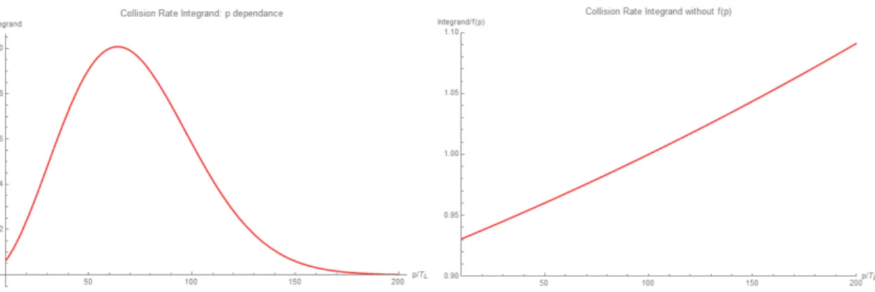
Figure 11:Left: The dimensionless integrand in equation 3.20. The integrand is heavily suppressed by f(p0) atp0 < 10 andp0 > 150, which will guide our choice of p0 when evaluating the integral to verify our approximations. The integral has been scaled to be between 0 and 1. Right: The dimensionless integral in equation 3.23, afterf(p) has been integrated out. We see that without f(p), the integrand only varies by about a few percent in the relevant range. Recall from the figure on the left that for p0 outside of the interval (10,150), the integrand is heavily suppressed. The integrand has been scaled so that it equals one at p0 = 100.

Γ = 1

nχ

Z _d3_p

2mχ

C

= C

210_π7_m4

χnχ

Z

d3p dP kp

∗4 e k 3 2− 1

2cos (θCM)

pp∗

∗

χ

|p_exh0(pe 2₎_| ×[1−g(ek)]g(k)f(p).

(3.20)

We found numerically that thef(p)contains the only significant pdependence in the integrand (see figures (11) and (12)). This means we can pull the rest of the integrand out of the pintegral, and just integrate the distribution functionf(p). The number density is defined as:

nχ≡

Z _d3_p

(2π)3f = 4π Z _dp

(2π)3p

2_{f ,} _(3.21)

so we can integrate pout and cancel then−χ1. We then make the following substitutions to make

the remaining integral dimensionless:

p0≡ p TL

k0≡ k

TL e

p0≡ ep TL

e k0≡ ek

TL

p∗0≡ p

∗

TL

(3.22)

Γ = CT

5

L 210_π7_m4

χ

Z

dk0d(cos (θi))dθCMdϕCM

k0(p∗0)4 e k0

3 2−

1

2cos (θCM)

pp∗

∗

χ

|p_exh0(pe 2₎_| ×[1−g(ek)]g(k).

(27)

0 1 2 3 4 n 10-5

10-4

0.001 0.010

Tn/T0

Relative Contribution of Terms ofpχ/mχTaylor Series

0 1 2 3 4 n

10-5

10-4

0.001 0.010

Tn/T0

Relative Contribution of Terms ofTL/mχTaylor Series

Figure 12: The Taylor series expansion of the integrand in equation 3.23. The left plot is an expansion in p0, and the right plot is an expansion inTL/mχ. Each termTn is

divided by the 0th order term T0, giving the fractional correction to the constant approximation we make in section 3.4. The first order terms of both expansions are corrections of 5-10%, and the following terms quickly vanish. These terms were calculated numerically, for fixed values of the other parameters, chosen from the typical ranges encountered in the simulation. Varying these parameter choices through the range of typical values has little effect on the magnitude of the expansion terms shown in this figure.

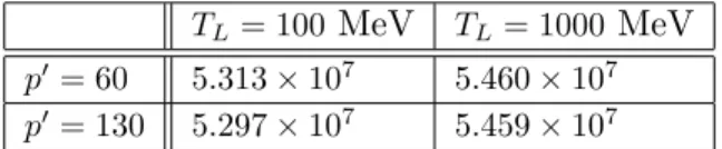
TL = 100MeV TL = 1000MeV

p0 = 60 5.313×107 ₅_.₄₆₀_×₁₀7 p0 = 130 5.297×107 ₅_.₄₅₉_×₁₀7

Table 1: The numerical solution for the dimensionless integral in equation (3.23) for several values of p/TL andTL. The two p/TL values are chosen from the lower and higher

ends off(p) shown in figure (11), and theTL values are chosen from the range of

(28)

It was found numerically that the remaining dimensionless integralI is not sensitive toTL. This,

along with the independence of the integral to the chosen value ofp0, is demonstrated in figure (12) and table (1). While there is small variation in the value of I, the deviation is less than 5%, and this effect will be neglected. The independence of I onTL means that it can be calculated

once, and the result is valid at all relevant times. Numerical integration givesI '5.3×107_{. We} can substitute in C as a function of the momentum transfer rate γ as given in equation 3.8 to compare to our order of magnitude estimate:

C=6048m

5

χ 155π3

γ T6

L

Γ = 6048mχγ 155×210_π10_T

L

I '21.57mχ

TL

γ.

(3.24)

We see that the order of magnitude approximation is correct to a constant correction of 21.57. While 21.57 is the number found here, the constant correction is in the next section empirically determined to be approximately 0.25. This discrepancy may be due to mistakes regarding constant factors in the above calculation, or possibly similar mistakes in the calculation of the matrix element by reference [25]. Such a mistake would not be unlikely. While γ has been used extensively, very few works have needed the absolute value of Γ before this, so any misplaced constant factors could likely go unnoticed.

Finally, we must findγ. We defineγ/H = 1 to be the kinetic decoupling temperature,Tkd. This is

whereγ drops belowH, meaning collisions stop having a significant impact on the dark matter momentum. We define one more temperature, the standard kinetic decoupling temperature, Tkds,

to be the decoupling temperature if we were in radiation domination. This gives γ(Tkds) =H(Tkds)RD. The energy density of relativistic particles is given by [24]:

ρr=

π2

30g∗T

4

L. (3.25)

Now that we have ρr, we can getH in radiation domination:

H =

s

8π

3m2

pl

ρr=

r

4π3

45 g∗

T2

L

mpl

. (3.26)

Evaluating this atTkds givesγ(Tkds). Since γ scales asTL6, we now have:

γ=

r

4π3

45 g∗

T2 kds mpl _T L Tkds 6 . (3.27)

Now we can use this in equation 3.24 to getΓ as a function of TL:

Γ = 21.57× r

4π3

45 g∗

mχ

mpl

T_L5 T4

kds

. (3.28)

Since TL is known from the numerical work in section 3.2, we now have the collision rate we need

(29)

2.4. Additionally, the simulation does not actually calculate the collision probability for a

timestep∆t, but rather the timestep required for a desired collision probability Pcoll. This results

in an adaptive step size; the simulation takes very small steps when there are frequent collisions, and larger steps when there are fewer collisions. Pcoll must be a very small number (chosen to be

0.0005 in this simulation) so that the probabilityP2

coll of two collisions occurring in a single

timestep is small.

3.5. Sampling Collision Parameters

To sample the collision parameters that determine the outcome of a dark matter - lepton collision (k,cos (θi),θCM, and ϕCM) we will use a Metropolis Hastings MCMC algorithm, with the target

distribution being the integrand of equation 3.19. The Metropolis Hastings algorithm samples distributions through a random walk process. Starting with an initial guess for the desired parameter, the algorithm takes many random steps, dictated by the target distribution. The sequence of steps is called a Markov chain. A simplified form of this algorithm in one dimension is shown in algorithm (1).

In a typical case, a distribution would be modeled by creating a very long Markov chain, and saving every step. The target distribution can then be sampled by selecting a step of the Markov chain randomly, with an equal chance of selecting any step. For our purposes, this is unnecessary and unrealistic. Every collision only needs a single sample from the parameter space, so

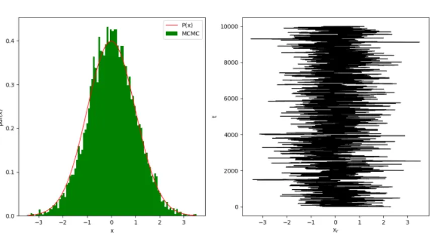
producing a full distribution that can be repeatedly sampled is far more work than is necessary. Furthermore, this process must be done in a four dimensional parameter space, and repeated for every collision, of which there are thousands. To make it even more unrealistic, that entire process is then repeated for thousands, even tens of thousands of particles. An example 1,000 step Markov chain of a normal distribution is shown in figure (13). This is a fairly well behaved distribution, and it still has visible accuracy issues at 1,000 steps. Additionally, the parameter space is four dimensional, so not only will each step take longer, but it will also need more steps for the random walk to accurately sample the space. This approach would clearly produce computational challenges that would significantly hinder the work. Fortunately, there is an alternative approach.

To sample a single point from the parameter space, we construct a relatively short Markov chain, and select the final point as our sample. The difficulty is that this chain must be long enough that the final point is entirely independent of the initial guess, otherwise the distribution from which the initial guess is drawn will be convolved with the target. On the other hand, the chain must be as short as possible in order to keep computation times reasonable. The minimum number of steps was determined empirically. To do this, we ran thousands of independent Markov chains, taking the final point of each. These final points were then plotted in a histogram, and compared to the analytical target distribution. Since the distribution is four dimensional, multiple two dimensional projections were examined to ensure accurate sampling. After adjusting the chain length and looking at the results for various values ofTL and p, it was

(30)

Algorithm 1:Producing a 1D Markov chain

Result: Create a 1D Markov chain with R entries for target function f tar. f tar is the probability density we are sampling values from. δ is a pre-chosen step

parameter based on f tar that can be optimized quantatively, but in our case is found through trial and error as the value that gives fastest convergence. x0 is the initial guess for the parameter. normal(mean,stdev) is a function that samples a normal distribution, and uniform(a,b) samples a uniform distribution from a to b.

n = 0 xnow =x0

whilen < R do

xtry =xnow + normal(mean=0, stdev=δ)

P1 = f tar(xnow) (sample target at current and proposed point)

P2 = f tar(xtry)

Q=P2/P1 (a measure of how much more or less probable the new point is than the last)

if Q >1 then

xnow =xtry (if the new step moves to a higher point in f tar, accept the step) else

N = uniform(0,1) (if the new step moves to a lower, point in f tar, there is a probability that it will still be accepted)

if N < Q then

xnow =xtry end

end

n+=1 (the Markov Chain advances whether the new point is accepted or not)

(31)

Figure 13: An example of a 1000 step Metropolis Hastings MCMC algorithm, used to sample a normal distribution with mean 0 and standard deviation 1. Left: a histogram of the Markov chain, with the target distribution superimposed on it. There are clear deviations from the target, namely an oversampling in the center and an undersampling on the left side. This is due to a small sample size - the errors are random and change between trials, and running 10,000 or more steps tends to give a more accurate realization of the target. Right: a plot of the Markov chain entriesxr

as a function of step number t. The algorithm clearly spends more time in the center of the distribution than out towards the edges, and when it does move far from 0 it is quickly reflected back.

4. Results

4.1. Single Particle Evolution

The simulated evolution of a single particle is shown in figure (14). We can see that at early times, beforeγ/H = 1, the momentum appears to be going as a−3/16. This corresponds to tight coupling between Tχ and TL: ifTχ∝TL∝a−3/8 and Tχ= 2₃h

p2i

2mχ, thenp∝a

−3/16_{. This is expected,} since at these early times there are enough collisions that the two populations should be tightly coupled. This is reflected in the bottom panel, where we see very dense collisions at the

beginning of the simulation. Betweenγ/H = 1 andΓ/H= 1 we see the frequency of collisions decreasing greatly, with the final collision occurring right around Γ/H= 1. While these results are promising, we must remember that the collision history of a single particle is random. To truly test this simulation we will need to run many more particles, and observe the ensemble behavior.

We can also test the prediction of appendix B, that in the limit of constantg∗ the Boltzmann

(32)

Figure 14: The evolution of a single dark matter particle. This simulation is for mχ = 125 TeV,

Tkds= 21.3 MeV, andTRH = 0.01 MeV.Top: the evolution ofp. Two lines are provided

as reference: p ∝ a−3/16_{, corresponding to tight coupling with}_T

χ 'TL, and p ∝ a−1,

corresponding to no collisions and only redshifting. Bottom: the individual collisions. Each vertical green line corresponds to one collision, and the vertical red line is the final scattering.

Figure 15: The fractional momentum change for each collision, withγ/H and Γ/H for reference. While there is significant scatter in dp/p, there is a clear trend that rises above 1 as