A functional dynamic factor model

(1)

A Functional Dynamic Factor Model

by

Spencer Eric Hays

A dissertation submitted to the faculty of the University of North Carolina at Chapel Hill in partial fulfillment of the requirements for the degree of Doctor of Philosophy in the Department of Statistics and Operations Research.

Chapel Hill 2011

Approved by:

Haipeng Shen, Advisor

Chuanshu Ji, Committee Member

Young K. Truong, Committee Member

Jianhua Huang, Committee Member

(2)

c

(3)

ABSTRACT

SPENCER ERIC HAYS: A Functional Dynamic Factor Model. (Under the direction of Haipeng Shen.)

(4)

func-tional dynamic factor model and areas of future research are described.

(5)

ACKNOWLEDGMENTS

I would like to acknowledge the contributions of, and my gratitude to, my advisor Professor Haipeng Shen. It is an understatement to say I could not have done this without his help. Of course the research content itself stemmed from his own research interests. Yet in addition, the fulfillment of this dissertation not only required his expertise in the subject matter but also his ability to serve as an exemplary mentor; and having done so amidst a myriad other responsibilities. It has been a true honor to work with him, I am proud to have done so, and I only hope I represent him well in my own research going forward.

I would also like to thank my committee members: Professors Chuanshu Ji, Young Truong, Jianhua Huang and Harry Hurd. I was fortunate to have a committee with members of such varied research interests; and with each a command of knowledge in both breadth and depth of subject matter area. This dissertation greatly benefitted from the confluence of their input, and of course their support. Their approval of the research proposal and subsequent recom-mendations set the foundation for this dissertation. I am grateful for their assistance in the completion thereof.

I thank my employers at the Department of Psychiatry: first and foremost Professor Hongbin Gu and Professor Bob Hamer. I learned my own research area from my dissertation, but from them I learned what it is to be a collaborative researcher and a career statistician: for this I am in their debt, and I can not thank them enough for the opportunity to have worked with them. I would also like to thank Janet Spear for her help and support; both with my work in Psychiatry, and for her support in all other regards. Finally I thank Ann VonHolle, Sandra Woolson, Jackie Johnson, Abby Scheer and Junghee Choi: their knowledge, support and camaraderie is unmatched; and I hope we can work together again in the future.

(6)

parents, John Hays and Patricia Hays, have been constant inspiration and support. For this I thank them. Likewise to my brothers Justin Hays and Zachary Hays, I have appreciated all of their help and guidance. Also with special thanks to Zachary’s wife and children; Brie Hays; Fletcher Hays and Kate Hays, respectively.

(7)

List of Tables

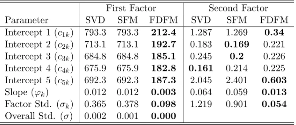
5.1 Parameter Bias and (Std. Dev.) for the case where σ = 2. Smallest bias (in magnitude) and standard deviation are indicated in bold. Despite comparable performance of SFM and FDFM on factor loading curves, FDFM estimation results in nearly uniform lower bias and standard deviation for first factor pa-rameters. For second factor estimates, FDFM produces lowest bias while for the majority of parameters SFM displays lower standard deviation. See Table 5.2 for reconciliation. . . 100

5.2 MSE for the case where σ = 2. Smallest MSE indicated in bold. FDFM esti-mates result in uniformly lower MSE for factor one parameters. Despite lower standard deviation of SFM factor two estimates (Table 5.1), the majority of FDFM estimates achieve lower MSE. . . 100

7.1 MFE and RMSFE: 1, 6, and 12 month ahead Yield Curve Forecast Results. The better result between the two models is highlighted in bold. For 1 month ahead forecasts, the FDFM results in lower (magnitude) MFE for most maturities but results are mixed for 6 and 12 months ahead. RMSFE is typically lower with the FDFM for 1, 6 and 12 months ahead. . . 140

7.2 Average RMSFE; FDFM as a fraction of DNS: (a) with Extrapolation (b) With-out Extrapolation . . . 142

7.3 Algorithm 1: Weighted Pairs. Use of the FDFM model results in nearly twice the cumulative profit produced from the DNS model. . . 144

7.4 Algorithm 2: Optimal Pairs Portfolio. . . 145

8.1 RMSE and APE For Call Data From SVD Model, FDFM Sequential (EM-Q), and FDFM Simultaneous (EM-S). The simulataneous method has the lowest mean and median RMSE and APE. Variability of forecasts are comparable be-tween the three methods. . . 152

(12)

List of Figures

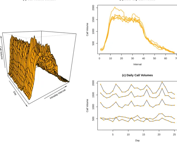
1.1 Example of Dynamic Functional Data. Three views of a functional time series. Panel (a) illustrates the surface created by plotting intraday call volumes by day. Panel (b) depicts cross sections of the data at five time points (days), resulting in a view of five intraday call volume profiles. These are hypothesized to consist of a smooth underlying curve and an error component that accounts for departures from smoothness. Panel (c) shows the daily time series of call volumes within a sample of five different 15 minute intervals. . . 3

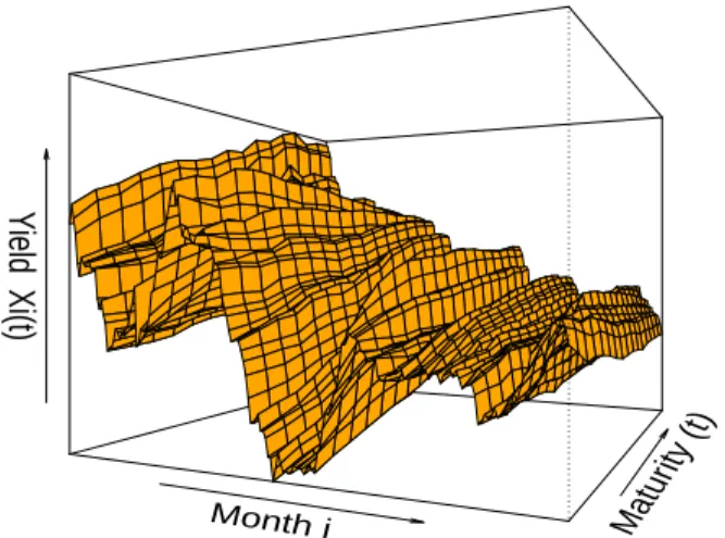
2.1 Example of Dynamic Functional Data. Data for yields xij on all observed

ma-turities tj at all datesiis plotted. . . 10

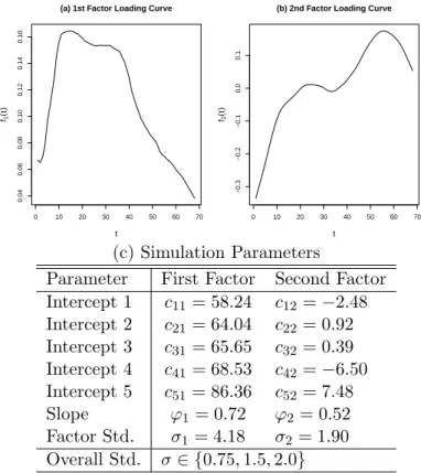
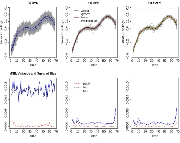
5.1 (a)-(b) Factor Loading Curves. Factor loading curves used to simulate the data are based on SFM estimates from the actual call center data. (c) Simulation Parameters. Parameter values are based on FDFM estimates of call center data. 97 5.2 Factor Loading Curve Estimates forf2(t) from the SVD, SFM, and FDFM

mod-els where σ = 2. The top row shows the estimated factor loading curves with mean and quartile bands. The second row shows the MSE, squared bias and variance. The FDFM produces much less variable estimates than SVD, while FDFM and SFM estimates are quite comparable. . . 98

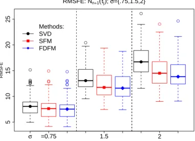
5.3 Forecast Performance. RMSFE based on Nij from Section 5.2.3 for the SVD,

SFM and FDFM models by the three values of σ. Asσ increases, the SFM and FDFM outperform SVD by a greater margin. . . 102

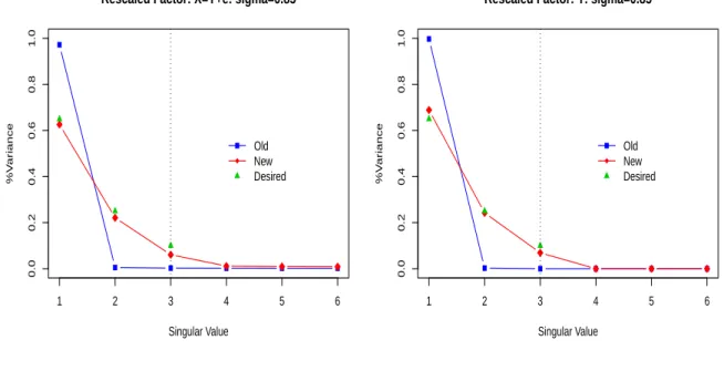
6.1 Example of Factor Re-scaling. We simulate data based on estimated parameters from the true yield curve data in Chapter 7 for 3 factors. Using the method described in Section 6.1, we re-weight the data by scaling the original singular values (blue) to form a new dataset. Those singular values (red) resemble the desired weighting (green). . . 106

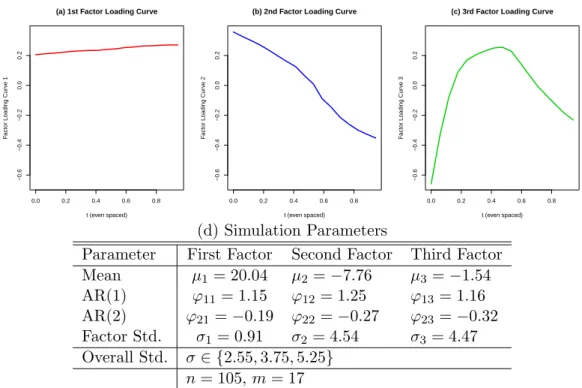
6.2 (a)-(c) Factor Loading Curves. Factor loading curves used to simulate the data are based on FDFM estimate actual yield curve data from Chapter 7. (d) Sim-ulation Parameters. Parameter values are also based on FDFM estimates of the yield curve data. . . 107

6.3 Example simulated data set according to the design in Figure 6.2. In grey are

(13)

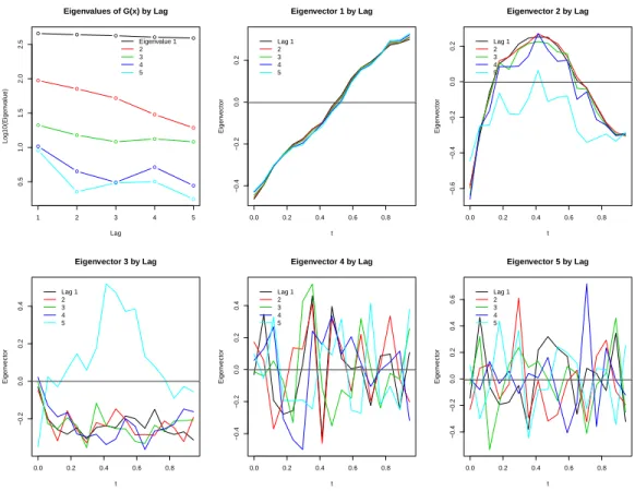
6.4 Eigenvalues and eigenvectors by lag l = 1, . . . ,5 for Gx(l), based on Pena and Box (1987). For simulated data consisting of 3 factors, the first 3 eigenvalues of the sample autocovariance matrix are large consistently across lags. For the 5 lags shown, the first 3 eigenvectors noticeably deviate from zero, indicating 3 factors. . . 111

6.5 True and estimated factors. For K=3 simulated data, the 3rd dynamic factor is plotted with AR(2) estimates (red points/line). The factor is then re-sampled and plotted (green points) with its AR(2) estimates. The re-sample destroys the dynamic dependence, thus resulting AR(2) estimates are close to zero. . . 113

6.6 Example “scree” plots for bootstrap approach. For a single simulated data set we examine singular values in terms of % of variance explained for the true data (red), the (K+ 1)st left singular vector and value replaced with AR(2) estimate (green), and mean over 200 bootstraps of resampled (K+ 1)st left singular vector and value replaced with AR(2) estimate (blue). For trueK = 3 factors, resample of second and third left singular vector and value affects singular values. . . 116

6.7 P-values and %Variance for Hypothesis Tests for the simulated data of 3 dynamic factors. Top: We reject the hypotheses of fewer than 2 and 3 factors, but are unable to reject fewer than 4 (and thus 5) factors. Bottom: Boxplots of ι(·)

corresponding to each test over all simulations for each choice ofσ. In blue, the average over 200 bootstraps forX∗; in green the values for ˆX. The first two plots confirm the result of zero p-values for tests of fewer than 2 and 3 factors (ι(2)

andι(3)_{,respectively); the third and fourth illustrate the large overlap in}_ι(4) _and ι(5) for testing fewer than 4 and 5 factors. . . 118

6.8 Canonical correlations for increasing number of series considered, by lag. Yield simulation design: K = 3 factors. As m increases – equivalent to a denser sampling – the decay in squared canonical correlations is more persistent. This inflates the test statistic of Pena and Poncela (2006), making rejection rare even when the number of factors being tested well exceeds the true numberK. . . 121

6.9 Canonical correlations for increasing number of series considered, by lag. Bathia et al. (2010) simulation design: K = 4 factors. We see the same pattern of slow decay in SCCs when m, the rate of sampling of a functional time series, grows large. . . 122

(14)

7.1 Example of factor loading curves: FDFM curves (solid, left axis) estimated from the period May 1985 to April 1994; pre-specified DNS curves (dashed, right axis). FDFM estimates closely resemble the shape of the DNS curves for the second and third factors, whilef₁F DF M resembles a typical yield curve shape. Dual axes have been utilized to account for difference in scale. . . 137

7.2 Example of Curve Synthesis: Entire time series of yields are omitted from esti-mation, then “filled in” using the imputation described in Section 4.3.3. Here, 3 consecutive maturities have been omitted, resulting in 3 missing time series corresponding to these maturities. . . 140

7.3 Algorithm 3: All combinations of portfolios for t2 > t1. The model with the

largest cumulative profit is displayed by the first initial of its acronym with “+” or “-” indicating positive or negative profit. . . 147

8.1 Day of Week Effect: intra-day and inter-day mean call volumes. In the top panel, mean call volume throughout the day shows a clear day-of-week effect. In the lower panel, the mean daily call volumes show a marked periodic effect. . . 150

8.2 Estimated Factor Loadings. EM methods result in smoother estimates due to the presence of a smoothing parameter. The first factor dominates. The greatest variability in estimates for the loading curves is exhibited in the simultaneous method, for which the reason may be slow convergence. . . 153

8.3 Forecasts by Day of Week. All methods are able to capture the day of the week effect. However all models also underpredict call volumes on Mondays, on average.154

8.4 Temperature and Pressure Data for El Nino Region . . . 155

8.5 Forecasts for the years 1986 (EN) and 1987 (SO) . In the top panel, the FDFM on the EN data closely resembles the ARIMA fit though is slightly closer to the actual data. The other functional models closely follow the pattern of the true data. In the lower panel are SO forecasts for the year 1987. All models produce similar forecasts and overestimate atmospheric pressure for the period April through October. Besides February, the FDFM performs at least as well as the other functional methods. . . 160

8.6 FDFM Forecast Performance on EN data. Panel (a) shows mean actual and mean forecast for the EN data 1987 through 1996. The model appears to fit quite well, however panel (b) shows the actual data is much more variable over the period than the FDFM forecasts. . . 161

(15)

Chapter 1 Introduction

Consider the problem of properly staffing a call center for, say, a major East coast credit card company. Call volumes fluctuate week to week, day to day, and even hour to hour. The danger of over-staffing is obvious: an overstaffed call center loses as much money as the idle employees are paid in hourly wages to (not) answer phones. The costs of an understaffed call center are more subtle but perhaps even more expensive in terms of customer affinity and attrition. By under-staffing, wait times for customers in queue are increased. In fact, call times are increased as representatives must take additional time to explain and apologize for the wait. As a result, customers can become dissatisfied with their product and cancel. Further increased demand on the fewer representatives leads to poor quality control. It is clear then, that non-optimal staffing is rather costly in either case. The solution is a forecast model that meets the specific needs of the call center environment.

An optimal staffing forecast model must take into account not only weekly call volume fluc-tuations, but also how volumes vary throughout the course of any given business day. The most mechanical way to develop a forecast model is to use the standard univariate auto-regressive, moving-average framework (ARMA). Supposing the data consist of quarter hourly volume mea-surements over dozens of weeks, an ARMA model could then forecast future call volumes by the hour, week, month, etc.

(16)

also exhibit a day of the week effect. Exceptionally long time series like this might also display the multiple seasonal components. In fact this is typical with this type of data (Taylor, 2008). Further, with the smallest data unit being a quarter hourly call volume, an ARMA model may be expected to forecast tomorrow’s volumes reasonably well. But for ”longer“ forecast horizons like even a few days ahead, the ARMA forecast would exhibit the usual mean-reversion seen in these models. Resulting in either over or under-staffing and the aforementioned costs associated with each of these. A better method to account for multiple periodicity would be to consider periodic auto-regressive models (PAR) (Hurd and Miamee, 2007). A connection to those types of models will be made in Chapter 6, however here, the method proposed is of a functional nature. It is a method capable of forecasting both within day (intra-day) call volumes and inter-day call volumes. A method that, similar to a PAR model, accounts for the multiple periodic components evident in the data. Consider the following proposed model, beginning with the actual data that motivated it.

Call volumes are recorded every fifteen minutes throughout the business day, resulting in 68 intra-day intervals. This data is collected over the course of 210 days. Because of the high frequency of the intra day call volumes, it is of interest to model these as a discrete sampling of a continuous process. That is, to picture a functional relationship for intra day call volumes on a given day as some smooth underlying curve plus a noise or error component (to account for departures from smoothness). Figure 1.1, panel (a) displays a portion of the actual call volume data to illustrate the idea of modeling the data as a time series of curves. Panel (b) illustrates an example of the functional view of the data. However, for a given time interval on each day it is also rather plausible that the volumes from that interval are related from one day to the next, as depicted in panel (c) of 1.1.

(17)

cor-Da y Intrada y Inter val Call V olume

(a) Call Volume Surface

0 10 20 30 40 50 60 70

500

1000

1500

2000

(b) Intra−day Call Profiles

Interval

Call V

olume

5 10 15 20 25

500

1000

1500

2000

(c) Daily Call Volumes

Day Call V olume ● ● ● ● ● ● ● ● ● ● ● ● ● ● ● ● ● ● ● ● ● ● ● ● ● ● ● ● ● ● ● ● ● ● ● ● ● ● ● ● ● ● ● ● ● ● ● ● ● ● ● ● ● ● ● ● ● ● ● ● ● ● ● ● ● ● ● ● ● ● ● ● ● ● ● ● ● ● ● ● ● ● ● ● ● ● ● ● ● ● ● ● ● ● ● ● ● ● ● ● ● ● ● ● ● ● ● ● ● ● ● ● ● ● ● ● ● ● ● ● ● ● ● ● ●

(18)

relational structure inherent in data that occurs over time. An alternative is to simply treat the data as multivariate time series.

FDA provides a framework to work with the functional observations of curves. However, for each intraday interval there is also a daily time series of call volumes for that interval. This is essentially a multivariate time series, and a very large one: the motivating data set contains 210 days of data with 68 intervals each day. Modeling all 68 intervals jointly is intractable; even an order one unrestricted vector auto regression (VAR(1)) for 68 series would require a 68×68 coefficient matrix. In terms of a restricted VAR model, developing meaningful linear

restrictions on 68 series may make a restricted VAR just as unwieldy. Aggregating the data into coarser intraday intervals would allow a method like vector auto-regressions directly, though at the expense of a loss of granularity in the intra day call volume profile. Further, the finer fifteen minute intervals are industry practice.

Therefore, consider an alternative approach. In the interest of dimension reduction, it would be helpful if the behavior of the 68 related time series could be explained via a smaller set of variables. Then that smaller set of variables could be modeled as a more manageable multivariate time series. This aspect of the problem lends itself to the realm of dynamic factor analysis (DFA) where the observed multivariate time series data can be explained via a smaller multivariate set of unobserved or latent factors, also following a time series process and related to the observed data through coefficients known asfactor loadings (Basilevsky, 1994). So-called dynamic factor models (DFMs) first appeared in the literature independently by Geweke and Singleton (1981), Engle and Watson (1981) and Molenaar (1985), and have enjoyed some success in problems involving either economics or psychology.

(19)

approach with natural cubic splines (NCS) to capture the functional behavior of the yield curve. The method was computationally intensive in that selection of the appropriate knot locations for the NCS’s used a goodness-of-fit measure on every possible combination of 3 to 4 internal knots out of 34 possible choices to determine the best model. In the latter case of four knots this requires fitting of 46,376 candidate models.

Ideally, a model to estimate and forecast functional time series like the call data should be both elegant in specification and estimation, and should further capture both the functional behavior and the time series behavior of the data. Therefore, what is proposed here is a synthesis of ideas stemming from both FDA and DFA to create a new model for the purpose of forecasting time series of curves. Presented in this dissertation is the specification of aFunctional Dynamic Factor Model (FDFM). The FDFM retains the idea of dimension reduction of the observed data into a more manageable set of unobserved time series factors, but further specifies that the factor loadings for each factor form a smooth curve. The hypothesis is that the observed data on a given day is the sum of a smooth underlying curve plus noise. The former component is then the sum of unobserved factors and their corresponding smooth factor loadingcurves.

Outside of the call volume setting, another application of the FDFM model is in reference to yield curve forecasting from Diebold and Li (2006) and Bowsher and Meeks (2008). Specifically, given a time series of zero coupon bond yields of multiple maturities (3, 6, 12 months etc.), it is of interest to forecast yields not only for bonds of the observed maturities but also for the entire curve or spectrum of maturities. This type of data lends itself exactly to the FDFM formulation. It further illustrates the importance of viewing the data unit as a curve and not just a collection of discrete data points. In an applied sense, though a particular maturity is not observed or even exists, it is essential to investors to have a yield measure for effectively any maturity in order to evaluate rates of return on portfolios of bonds with varying maturities. The functional perspective is advantageous from a statistical point of view as well. For example, modeling high frequency data as smooth curves results in a method robust to outliers (not that extreme events are unimportant, rather just in this context there is not a particular interest in them).

(20)

it can just as easily be applied to other time series. Consider for example, strongly seasonal climatological data such as sea surface temperature (SST) in the South Pacific. The El Nino phenomenon is a well documented cycle that strongly influences sea surface temperatures. Given a time series of monthly average SSTs, a natural method for estimating and forecasting the data is to model it simply as a univariate seasonal ARIMA model with period twelve. A better method may be to consider a PAR formulation given the strong seasonal nature of the data. However in the present context, another method is to consider the seasonal pattern as a sampling of an underlying smooth curve. That is, to reconstruct the long series of monthly single observations as an annual series of multivariate data with twelve observations per year. Then for each multivariate observation treat those twelve observations as a realization of a smooth underlying seasonal cycle plus noise. Put another way, the twelve months represent the discrete sampling from the underlying curve and then the data can be viewed as anannual

time series of curves that represent the cycle. Besse et al. (2000) used versions of functional autoregressive models (FARs) to forecast the data, but the data can just as easily be modeled within the FDFM framework.

Specification of the FDFM begins within the typical dynamic factor model framework. Errors are assumed to be normally distributed, and in the cases presented below, independent. The factors themselves are represented by low dimensional time series. In this dissertation, the cases presented are independent auto-regressive time series with no moving average components. This permits a straight forward derivation of a likelihood function. To ensure that the estimated factor loading curves are indeed curves, roughness penalties with smoothness parameters are added to the log-likelihood corresponding to each loading curve. By doing so, maximization of the penalized log-likelihood is a balance between goodness-of-fit and the smoothness of the loading curves. The smoothing parameters themselves are assumed as fixed but unknown, so a generalized cross validation approach is used to select those.

(21)

Expectation Maximization algorithm (EM) first introduced by Dempster et al. (1977). Meng and Rubin (1993) further derived the theoretical and convergence properties of the EM. The EM is an iterative procedure that begins with the specification of initial values for the factors and factor loadings, then each iteration of the EM involves an E-step and an M-step. In the E-step, conditional expectations of the factors given the observed data are used in place of the latent factors. In the M-step these conditional expectations are used in the maximum likelihood solutions (MLEs) to solve for the factor loading curves and other model parameters.

(22)

Chapter 2 Functional Dynamic Factor Model

This chapter develops the model by beginning from a functional perspective of the process gen-erating the data. Observed data is treated as a sampling of the underlying smooth functions and forms a data matrix. From this point the dynamic factor model framework is implemented hypothesizing the larger data matrix is composed of a smaller set of unobserved dynamic fac-tors following independent time series processes, and corresponding factor loadings. Imposing structure on the factor loadings so that they form smooth curves is the defining feature of the FDFM and relates the typical DFM model back to the functional domain.

To estimate the model a likelihood function can be derived based on the error assumptions. Then conditions on the proper amount of smoothness in the factor loadings facilitate a penal-ized likelihood expression. A detailed description of the use of the Expectation Maximization algorithm to estimate the model follows, including specific solutions for the maximum likeli-hood estimates (MLEs). Next, certain computational efficiencies are highlighted in regards to implementation. Finally, some alternative models are discussed.

2.1 The Model

Development of the model begins with a description of the data and its associated notation. Consider a time series of curves {xi(t) : t ∈ T;i = 1, . . . , n}, where T is some continuous

(23)

underlying curve, yi(t); plus an error component,i(t):

xi(t) =yi(t) +i(t). (2.1)

The purpose of this dissertation is to develop a viable model capable of forecasting the entire smooth curve for some future date: yn+h(t) withh >0, of course.

A good example of this type of process is the yield data introduced in the first chapter. Here

xi(t) would represent the yield to maturity as of date i for a (zero coupon) bond of maturity

t. In financial terms, it is useful to investors to have information about the entire continuous yield curve. But of course in practice, yields are only observed for a discrete class of maturity horizons; 3 months, 6 months and so forth. This is also the case of the general problem in this dissertation: that only distinct data points are observed, yet the intent is to work with and forecast the entire curve over time.

Specifically, for t ∈ T, consider a sample of discrete points {t1, t2, . . . , tm} with tj ∈ T for

j∈ {1, . . . , m}. Then denote:

xij ≡xi(tj).

In other words, from an FDA perspective, the observed data xij is a point sample from the

process xi(t) at the specific value t = tj. With the discrete values of the data, they can be

collected into a data matrix which is the starting point for the Factor Analysis component of the model specification.

Specifically, for the observed data{xij :i= 1, . . . , n;j= 1, . . . , m}, letiindex the row, and

j index the column of a data matrix Xn×m so that the i, jth element of X isxij. In reference

to the yield example, the rows ofX correspond to yield curves for at a fixed date; the columns are the time series of yield for a specific maturity. Figure 2.1 is a visual representation of a data matrixX.

2.1.1 The Classical Dynamic Factor Model

(24)

Month i _Matur ity (t)

Y

ield Xi(t)

Time Series of Yield Curves

Figure 2.1: Example of Dynamic Functional Data. Data for yieldsxij on all observed maturities

tj at all datesi is plotted.

first step then is to reduce the dimensionality of the problem via the use of dynamic factor modeling. The idea is that the behavior of a set of m observed variables can be explained through the behavior of a much smaller, though unobserved, set of K variables or factors and their corresponding coefficients called factor loadings. To capture the dynamic nature of the data it is postulated that the latent factors themselves follow a stochastic process. Later constraints will be placed on the model so that the factor loadings form smooth curves.

Following the notation of Pena and Box (1987), denote the rows of X as m×1 column

vectors xi, the general dynamic factor model can be represented in the following form:

xi = F0m×Kβi+i, (2.2)

i ∼ Nm(0,Σ),

wherexi is the vector of observed data at timei,i= 1, . . . , n;Fis a fixed but unknownK×m

(25)

and i = [i,1, . . . , i,m]0 is a Gaussian error vector with a full rank covariance matrix Σ.

The factors are hypothesized to follow a K-dimensional vector auto-regressive moving av-erage (VARMA(P,Q)) process. Using the lag or back-shift operator Lpβ_i = β_i−p (Hamilton,

1994), the multivariate factor time series can be modeled as

Φ(L)β_i = Θ(L)vi, (2.3)

vi ∼ NK(0,Σv),

with

Φ(L) = IK−Φ1L−. . .−ΦPLP,

Θ(L) = IK−Θ1L−. . .−ΘQLQ.

TheK×KΦ and Θ coefficient matrices are assumed to be such thatβ_iis a covariance stationary vector time series. Finally, identification of the model requires further assumptions typically on either the structure of the covariance matrix Σv or on the properties of the factor loadings;

the particular restriction employed here is discussed in the next section.

2.1.2 The Functional Dynamic Factor Model

Two types of additional assumptions are added to (6.1) and (2.3) to form the Functional Dynamic Factor Model; those that make this a functional model and those that are intended to simplify the development of the FDFM. The latter of these are discussed first.

These additional assumptions may be relaxed at a later time in order to provide a more gen-eral model framework. They are imposed here if only to provide a more parsimonious endeavor into this new, exciting class of models (see Chapter 9 for possible extensions). Specifically:

1. The K dynamic factorsβ_i have no moving average components (Θ(L) =IK).

(26)

3. Σε=σ2Im.

4. The innovations i and vi+h are uncorrelated at all leads and lags (h= 0,±1,±2, . . .) for

all k∈ {1, . . . , K}; allj ∈ {1, . . . , m}.

5. For the purposes of the proposed model it will be assumed that the loading vectors inF

are orthonormal: FF0 =Ik.

6. (Optional) Due to the simplified univariate AR structure and for additional flexibility, in place of a constant, non-stochastic regressors can be considered in the factor time series.

With these simplifying assumptions the FDFM can be expressed in the following scalar manner. Denotefkj as the kjth element ofF. Then implementing these assumptions, together

with (6.1) and (2.3), yields the model:



       

       

xij =PKk=1βikfkj+ij, ij

i.i.d.

∼ N(0, σ2)

βik−Aikµk=

Ppk

r=1ϕrk(βi−r,k−Ai−r,kµk) +vik, vik i.i.d.

∼ N(0, σ2_k)

Evtksj = 0 for t, s= 1, . . . , n; k= 1, . . . , K; j= 1, . . . , m,

(2.4)

where for date i, the 1×dk regressor vector for the kth factor is Aik, with dk×1 coefficient

vectorµk. Going forward, this will be denoted as an FDFM(K,p)model, which refers to theK

factors and the orderp= max{p1, . . . , pK} of the auto-regressive factors.

(27)

Specifically, let

F=



    

f1

.. .

fK



    

(2.5)

withfk= [fk1. . . fkm] so that fk is the sequence of factor coefficients corresponding to the kth

factor. Then based on the fifth assumption above, this implies

fkfl0 =



 

 

1 ifk=l,

0 otherwise.

(2.6)

Recall the original formulation of the observed data as a sample of a continuous process; that the observed dataxij is a point sample from the processxi(t) at the specific value t=tj.

Since xij = PKk=1βikfkj +ij, it is proposed that the factor loadings are themselves discrete

samples from continuous, unobservedfactor loading curves. That is, thatfkj ≡fk(tj) and that

eachfk represents the sampled curve corresponding to thekth factor. Thus, while the dynamic

factors represent a time series at discrete time points i ∈ {1, . . . , n} the factor loadings are a realization of a continuous function evaluated at m distinct points. It is precisely here where the synthesis of functional data analysis and dynamic factor models occurs.

xi(tj) =

K

X

k=1

βikfk(tj) +i(tj). (2.7)

This closely resembles the formulation of a classical dynamic factor model if not for the func-tional assumption on the factor loadings.

2.2 The Joint Distribution

(28)

is discussed in the next section, followed by a rigorous development of the EM implementation. The remainder of the dissertation includes many mathematical derivations and thus the introduction of some matrix notation will be useful hereafter. The modelxij =PK_k₌₁βikfkj+ij

is represented in matrix form as

Xn×m=Bn×KFK×m+n×m, (2.8)

whereB={mβik}= [β1. . .βK] and βk = [β1k. . . βnk]0.

For the moment, suppose the values of the factor time series are known. If this is the case then finding the joint distribution of the observed data and the factors is a fairly straightforward exercise and consists of the distribution for the factor time series and the distribution for the observed data. That is, the distribution of X and B is found by finding the conditional distribution of X given B, and the unconditional distribution of B. The latter is determined using the familiar properties of univariate autoregressive time series which aids in the derivation of the former.

2.2.1 Distribution for the factor time series

With the independence assumption for the factor time series from Section 2.1.2, the joint distribution for the factor time series is just the product of the univariate time series. Each univariate distribution is then the product of an unconditional distribution for the firstpvalues of the factor and the distribution conditioned on those pvalues.

For notational convenience and without loss of generality, for the following derivation it is assumed that:

1. no regressors are included in the time series other than an intercept for each of the K

factors.

2. It is further assumed that the order of the AR(pk) processes are the same for all factors.

That is, pk≡p∀k.

(29)

is defined asp= max{p1, . . . , pk}then it is easy to imagine that corresponding coefficients ϕrk

are simply set to 0 for r ≤ pk < p. For the former assumption, the model equation for βk

in (2.3) simplifies to

βik =ck+

p

X

r=1

ϕrkβi−r,k+vik ; fork= 1, . . . , K.

Since theKfactor time series are assumed to be independent, their joint distribution factors to the product of the univariate distributions for the time series:

f(B) =f(β₁, . . . ,β_K) =

K

Y

k=1

f(β_k). (2.9)

Each univariate distribution in the expression above can be further decomposed via conditioning on the firstp observations (Hamilton, 1994). Consider the likelihood for the factor time series

β_k as

f(β_k) = f(β1k, . . . , βnk)

= f(β1k, . . . , βpk)f(βp+1,k, . . . , βnk|β1k, . . . , βpk)

= f(β1k, . . . , βpk)







n

Y

i=p+1

1

q

2πσ_k2 exp

−(βik−ck−

Pp

r=1ϕrkβi−r,k)2

2σ2

k





 ,

which can be substituted into (2.9) to obtain the likelihood for the factor time series.

2.2.2 The Joint distribution and Likelihood of X and B

The joint distribution ofXandBcan similarly be simplified via successive conditioning. Using the property thatij

iid

(30)

Proposition 2.2.1. Joint Distribution of X and B

f(X,B) =

K

Y

k=1

f(β_k)×

n Y i=1 m Y j=1

f(xij|βi1, . . . , βiK)

=

K

Y

k=1

f(β1k, . . . , βpk) (2.10)

× K Y k=1    n Y

i=p+1

1

q

2πσ_k2 exp

−(βik−ck−

Pp

r=1ϕrkβi−r,k)2

2σ2

k    × n Y i=1 m Y j=1 1 √

2πσ2exp

"

−(xij −

PK

k=1βikfjk)2

2σ2

#

.

Finally, the log-likelihood expression is achieved by applying the natural logarithm to the above joint distribution, then multiplying by −2,

(−2×) lnL = −2

K

X

k=1

ln[f(β1k, . . . , βpk)] + (n−p)

K

X

k=1

ln(2πσ2_k) +nmln(2πσ2) (2.11)

+ 1 σ2 n X i=1 m X j=1

(xij − K

X

k=1

βikfkj)2

+

n

X

i=p+1

K X k=1 1 σ2 k

(βik−ck− p

X

r=1

ϕrkβi−r,k)2.

For the auto regressive parameters, the independence assumption on the time series factors allowsK distinct optimization problems for each of theKfactors. However, note the appearance of the term

K

X

k=1

ln[f(β1k, . . . , βpk)].

This is the log sum of the joint distributions for the first p time points for each factor. Op-timization including this term would require numerical methods, so for ease of computation a conditional likelihood approach is employed where [β1,k, . . . , βp,k]are assumed as known/given

for all k.

Notwithstanding some miracle, optimization of the likelihood (2.11) would generally not result with estimates of the {fk} resembling smooth curves. Therefore, some additional work

(31)

this is addressed in the next section.

2.3 The Penalized Likelihood Expression

Simply finding the optimal solutions to the likelihood expression (2.11) falls short of fully estimating the functional DFM on two counts. First, the factor time series are unobserved. Second, there is no reason to expect that by finding the values of the factor loadings and other parameters that maximizing the expression above will in any way satisfy the prior assumption that the factor loadings represent smooth curves. The latter is discussed presently; the former in the section on estimation.

From the likelihood (2.11), a maximum likelihood solution for the factor loading curves is equivalent to a minimization of the sum of squares

n

X

i=1

m

X

j=1

"

xij−

K

X

k=1

βikfkj

#2

=

n

X

i=1

m

X

j=1

"

xi(tj)−

K

X

k=1

βikfk(tj)

#2

,

with respect to the functions{fk(·)}.

It is proposed to follow the roughness penalty approach of Green and Silverman (1994), where a roughness penalty with a smoothing parameter is added to the sum of squares. In the functional dynamic factor model, for each of the K factor loading curves, K roughness penalty/smoothing parameter terms are added to the sum of squares. Consider the following penalty criteria for each of the factor loading curves: λk

R

[f_k00(t)]2dt. Then thepenalized sum of squares becomes:

n

X

i=1

m

X

j=1

(xij− K

X

k=1

βikfkj)2+

K

X

k=1

λk

Z

f_k00(t)2dt.

These terms place a condition on the second derivative of each functionfk. In this context

this is equivalent to a condition on the curvature of the function, which specifies that on the domain of the function, it is not too “rough.” The coefficient λk controls how strictly this

(32)

those that would lie along the smooth underlying curve.

In practice, first and second differences are used to approximate the first and second deriva-tives offk(·). Green and Silverman (1994) showed these are actually equivalent in the setting

of the natural cubic spline (NCS). This result is yet to be shown here, but is addressed in Chapter 9. In the meantime, just as a matter of practical implementation, first differences can reasonably approximate first derivatives and second differences can likewise approximate second derivatives. With ∆ representing the difference operator ∆fkj =fkj−fk,j−1:

λk

Z

f_k00(t)2

dt ≈ λk

m−1

X

j=2

∆2fkj

∆2_t

j

2

.

So, for example, if the pointstj are evenly spaced, then ∆tj = 1, and

λk

Z

f_k00(t)2

dt ≈ λk

m−1

X

j=2

[fk,j−1−2fk,j+fk,j+1]2.

Coefficients from this sum can be collected in the banded matrix

ω0_k ≡

               

0 . . . 0

1 −2 1 0 . . . 0

0 1 −2 1 0 . . . 0

..

. . .. ...

0 . . . 0 1 −2 1

0 . . . 0

                .

LetΩk≡ωkωk0; then

λk

m−1

X

j=2

(33)

Next, using the vec(·) operator, which stacks the columns of a matrix, yields

K

X

k=1

λk

Z

f_k00(t)2dt ≈

K

X

k=1

λkfkΩkfk0

= vec(F0)0·S·vec(F0),

whereSmK×mK is the block diagonal matrix withm×mblocksλkΩk. Adding this term to the

portion of the log-likelihood creates a roughness penalty for each of the factor loading curves so that optimal solutions for the curves will reflect the dual objectives of both finding estimates that fit the data and ensuring those estimates exhibit an appropriate level of smoothness.

Combining the log-likelihood (2.11) with the K additional penalty terms results in the Penalized Log Likelihood expression

P L = −2

K

X

k=1

ln[f(β1k, . . . , βpk)] + (n−p)

K

X

k=1

ln(2πσ_k2) +nmln(2πσ2) (2.12)

+ 1

σ2

n

X

i=1

m

X

j=1

(xij− K

X

k=1

βikfkj)2

+

n

X

i=p+1

K

X

k=1

1

σ2

k

(βik−ck− p

X

r=1

ϕrkβi−r,k)2

+

K

X

k=1

λkfkΩkfk0.

2.4 Maximum Likelihood Estimation with EM

(34)

2.4.1 A Brief Overview of Maximum Likelihood with the EM

Expression (2.12) facilitates the use of ML to estimate the model parameters. These are the time series slopes, intercepts, and variances for each factor, the factor loading curves, and the overall model variance; collectively these will be referred to in the set Θ:

Θ≡

(

σ2,{

K

[

k=1

fk, σk2, ck, ϕ1,k, . . . , ϕp,k}

)

. (2.13)

Obviously, direct maximum likelihood estimation is only of use if there is data available with which to compute the estimates. In the present context of the functional dynamic factor model this is only partially the case as it is hypothesized the observed dataX is a function of unobserved explanatory factorsB. Thus despite having a theoretical solution for the parameter and factor loading estimates, the problem is as yet intractable due to the latent data. Therefore, the method is to treat this as a problem of missing data; enter the EM algorithm.

First introduced by Dempster et al. (1977), the EM is a method by which to impute missing data with values based on a conditional expectation using the observed, non-missing data. Further work by Meng and Rubin (1993) showed the theoretical properties of EM estimates, including the desirable properties regarding convergence. The current setting differs due to the inclusion of the penalty terms in the likelihood and so it is as yet undetermined if those results hold here. Further discussion on this point is reserved for future work in Chapter 9.

EM estimation is an iterative procedure; inaugurated with initial values, the algorithm then oscillates between the so-called E-step and M-step. It proceeds thusly:

Step 0: Initial Values: To initialize the EM algorithm, some form of starting values are required. Many possibilities exist, but here it is proposed that the right and left singular vectors extracted via the singular value decomposition (SVD) of the data matrix X will provide adequate initial estimates for the factors and loadings. Details will follow, but for now from these primordial time series and curves, parameter estimates may be calculated with which to inaugurate the E-step. Section 2.4.2 briefly covers this.

(35)

expectations given the observed data using the parameter estimates from either Step 0 or the previous M-step. The conditional expectations then take the place of the factor time series in the calculation of the factor loading curves and the next iteration of parameter estimates. See Section 2.4.3 for a thorough derivation.

The M-step: Based on the factor scores from the conditional expectation in the E-step, MLEs are calculated for the factor loading curves and other parameters using the ML solutions in the subsequent sections. The optimal solution for the set of{fk} is dependent on the

smoothing parameters{λk}, so as part of the M-Step the optimal solutions for the fk are

calculated based on several different values ofλk. A Generalized Cross Validation (GCV)

procedure is then used to select the optimalλk/fk pair. See Sections 2.4.4 and 2.4.5 for

details.

After the initial step, the E-step and the M-step are repeated until differences in the esti-mates from one iteration to the next are sufficiently small. See Chapter 9 for a discussion of convergence properties.

2.4.2 Step 0: Preliminary Estimates via SVD

Initial values for the factors and factor loadings are required to begin the EM. From those initial values, the variance and autoregressive parameters are calculated to inaugurate the E-step. Choices can be fairly arbitrary, but because of the connection of the functional dynamic factor model with other functional data analysis models (Shen and Huang (2005); Shen and Huang (2008); and Shen (2009)), singular value decomposition (SVD) is utilized on the original

X data matrix for preliminary estimates of the factor time series and factor loadings.

First, X is decomposed by SVD into three matrices. Two of which are the orthogonal matricesUandVwhich contain the left and right singular vectors respectively;U0U=V0V=

(36)

the diagonal. Hence, the SVD of Xis as follows:

X SV D= Un×mDm×mV0m×m

=

u1 . . . um



    

d1 0

. ..

0 dm



    



    

v₁0

.. .

v0_m



    

=

m

X

j=1

djujvj0.

Next, based on the model formulation that X is represented by K factor time series plus noise, the first K SVD components{dk,uk,vk}Kk=1 can be used to approximate X as in X ≈

PK

k=1dkukv0k. Let the (0) subscript denote the step 0 EM values. Then the initial values

for the factors and factor loading curves are designated as β_(0);_k = dkuk and f(0);k = v0k, for

k= 1, . . . , K. From these, initial parameter estimates are computed forσ2 and the set of factor

parameters {σ2

k, ck, ϕ1,k, . . . , ϕp,k} as described below in Lemma 2.4.1 and Equations (2.14)

and (2.15). Hence with starting values in hand, the true EM iterations can begin.

The next paragraphs briefly detail some of the maximum likelihood solutions to the penalized log-likelihood (2.12), beginning with the error variance, then the factor time series parameters. These are required to calculate the conditional mean and variance used in the E-step. For the moment, the smoothing parameters{λk} are taken as given; Section 2.4.5 details a generalized

cross validation approach for their selection.

The solution for the error variance, σ2, is as follows. The penalized log-likelihood (2.12) is differentiated with respect toσ2. Setting the resulting expression equal to zero, and solving for

σ2 _{results in the following MLE for} _σ2_:

ˆ

σ2 =

P

i,j(xij −PKk=1βikfkj)2

nm . (2.14)

Recall the assumption that the first p values for each of the factor time series are assumed as given. Then solutions for the AR(p) parameters reduce to an ordinary least squares problem. Holding the {σ_k2} fixed for the moment, maximization of (2.12) with respect to the {ϕk} and

(37)

Lemma 2.4.1. Define SSE=Pn

i=p+1

PK

k=1(βik−ck−Prp=1ϕrkβi−r,k)2, and let

yk ≡ [βp+1,k, βp+2,k, . . . , βnk]0,

Wk ≡



       

1 βp,k βp−1,k . . . β1,k

1 βp+1,k βp,k . . . β2,k

..

. ... ... . .. ...

1 βn−1,k βn−2,k . . . βn−p,k



       

(n−p)×(p+1) ,

and φk ≡ [ck, ϕ1k, ϕ2k, . . . , ϕpk]0.

ThenSSE =PK

k=1kyk−Wkφkk2 and for each kthe MLEs for the auto-regressive parameters

are the OLS solutionsφˆk= [W0_kWk]−1W_k0yk.

Alternatively, because of the independence assumption, all of the AR(p) parameters can be solved for simultaneously by posing the problem as one of multivariate regression.

Finally, with all of the estimates ˆφ, the individual variances can be found by differentiating the penalized log-likelihood (2.12) with respect to σ_k2, then setting the result equal to zero and finally solving for σ_k2:

ˆ

σ2_k =

Pn

i=p+1(βik−ck−Ppr=1ϕrkβi−r,k)2

n−p . (2.15)

With these initial parameters, the E-step can begin to update the values for the factors. Then the M-step is employed to update the values for the factor loading curves and other parameters.

2.4.3 The E-Step

(38)

Obviously, the E-Step of the EM requires the derivation of the conditional distribution of the factors with regards to the observed data. Restating the model terms of vector notation (as opposed to the matrix formulation), and due to the assumption of normality, the procedure is simplified. With the latter point the distribution is equivalent to the derivation of the first two moments; with the former, said derivation is forthright. To ease in the derivations, however, first consider the following lemma relating thevec(·) operator to the kronecker, or direct product:

Lemma 2.4.2. (Magnus and Neudecker, 1999). Let Γ and ∆ be two matrices such that the product Γ∆ is defined. Then

vec(Γn×K∆K×m) = ∆0⊗In

vec(Γ). (2.16)

Based on the lemma, the model (4.3) can be rewritten in a vector-ized form, which facilitates the distributional derivations. Let X ≡ vec(X) and β ≡ vec(B). Then the model (4.3)

X=BF+can equivalently be written as

X = (F0⊗In)β+vec(). (2.17)

Derivation of the conditional moments requires the expressions of some of the unconditional moments. Namely, these are:

1. The means of X and β, denoted as µX and µβ, respectively.

2. The variances of X and β, denoted as ΣX and Σβ, respectively.

3. The covariance of X and β, denoted as Σβ,X.

These moments in turn are dependent upon the errors associated with the time series factors and the model error .

First consider the variance matrix for each factor time seriesβ_k. Recall from Equation (2.9) that for the purposes of this dissertation it is assumed all theKfactors follow an AR(p) process of the form βik = ck+Ppr=1ϕr,kβi−r,k+vik. Then following Hamilton (1994), the following

(39)

Lemma 2.4.3. Let β1,k, . . . , βn,k follow a covariance-stationary AR(p) process represented

by βik = ck +

Pp

r=1ϕr,kβi−r,k +vik; with vik iid

∼ N(0, σ2_k) for i = 1, . . . , n. Define γk,s =

Cov(βik, βi+s,k).

Then

E[βik] =

ck

1−(Pp

r=1ϕr,k)

,

and

γk,s=



 

 

ϕk,1γk,s−1+ϕk,2γk,s−2+. . . ϕk,pγk,s−p for s= 1,2, . . .

ϕk,1γk,1+ϕk,1γk,2+. . . ϕk,1γk,p+σ2k for s= 0

.

Define then×nvariance matrix forβ_kas Σk. Its elements are then [Σk]h,i=γk,|h−i|. These results give rise to the unconditional moments forX andβ which are collected in the following proposition.

Proposition 2.4.1. Recall from the Equations (2.4)that ij ∼N(0, σ2). Then

V ar[vec()] =σ2Inm.

Further, let c be the K×1 vector with elements ck/[1−(Ppr=1ϕr,k)]. Then

µβ = c⊗1n

µX = (F0⊗In)µβ

Σβ = diag{Σ1, . . . ,ΣK}

ΣX = (F0⊗In)Σβ(F⊗In) +σ2Inm

Σβ,X = Σβ(F⊗In).

(40)

Proposition 2.4.2. Let



 

β

X 



 ∼ N



 



 

µβ

µX





,



 

Σβ Σβ,X ΣX,β ΣX



  



.

Then

µ_β|X≡E[β|X] = µβ+ Σβ,XΣ−X1(X −µX),

and

Σβ|X≡V ar[β|X] = Σβ−Σβ,XΣ−X1ΣX,β.

This then implies that

E[ββ0|X] = Σβ|X+µβ|Xµ0β|X.

Note that from a computational standpoint there is concern over the appearance of Σ−_X1 in the expressions for bothµ_β|X and Σβ|Xsince this is an inversion of order nm; because the EM is an iterative procedure, this could be especially problematic (recall the call center data with

n = 210 and m = 68). Thankfully, there is a method by which the inversion can be reduced to K sequential n×n inversions. This and more computational efficiencies are discussed in Section 2.4.6.

With these conditional moments, the E-step of the EM posits that the missing data (the time series factors) are replaced with the known values of the conditional distribution givenX. Thus in the M-step, in solving for MLEs, expressions involvingβ_k will utilize values fromµβ|X, Σ_β|X, and E[ββ0|X].

2.4.4 The M-Step

(41)

be determined using the surrogate conditional moments µ_β|X, Σβ|X, andE[ββ0|X] in place of the missing factor time series,β_k. In fact, the crux of the E-step/M-step transition is replacing the unknown factor terms in MLE solutions with the corresponding known terms from the conditional expectations.

To do this requires some overhead in terms of notation and some minimal derivation; bear with it, it’s worth it. Recall the set Θ from Equation (2.13); and denote the lth EM itera-tion parameter estimates as Θ(l). For each iteration l, the M-step optimizes the conditional

penalized log-likelihood (2.12) given the observed data and thelth parameter estimates:

E[P L|X]|Θ(l) ∝

1

σ2

X

i,j

E "

(xij − K

X

k=1

βikfkj)2

X

#

|Θ(l)

(2.18)

+

n

X

i=p+1

K

X

k=1

1

σ_k2E

"

(βik−ck− p

X

r=1

ϕrkβi−r,k)2|X

#

|Θ(l)

+

K

X

k=1

λkfkΩfk0.

As a matter of notation, where necessary, parameters or random variables will be suffixed with a value indicating the relative iteration of the EM; 0 represents the initial values andl= 0, . . . , L

represents the current iteration of the EM.

Based on the above expression, it is clear that in the MLEs, the factor time series appear either singly or in terms of cross products. Further, the cross products occur either within or between factors. These three variants, and the corresponding replacements are made thusly:

Individual factors: The conditional mean of the vector-ized factors, µβ|X, consists of the conditional means of each factor: [E(β₁|X)0_n_×₁, . . . , E(β_K|X)0]0. Thus for each time point

i and each factor k, βik;(l) is replaced with the ith element of factor k’s conditional

expectation, [E(β_k|X)]i.

Within factor cross products: For a given factor k, and time points i, h = 1, . . . , n, then [βikβhk](l) =E[βikβhk|X]. An exciting result is that Σβ|X is block diagonal withK n×n blocks. Therefore,E[βikβhk|X] is simply thei, jth element of thekth diagonal block from

(42)

Between factor cross products: For a given factors k and k0; and some given time points

i, h = 1, . . . , n; the replacement is [βik0β_hk]₍_l₎ = E[β_ik0β_hk|X]. An even more amazing

result is thatE[βik0β_hk|X] is simply thei, jth element of the matrix formed by [E(β_k|X)]·

[E(β0_k|X)]0. Put another way,the conditional expectation of the product is just theproduct of the conditional expectations. For a derivation of this see Chapter 3.

The M-step, then, is just a matter of making these substitutions into (2.18), and solving for the MLEs. For ease of notation, going forward it will be implicit in the expressions and derivations that items like βik orβikβhk0 are equivalent toE[β_ik|X] and E[β_ikβ_hk0|X],

respec-tively; for i, h= 1, . . . nand k, k0 = 1, . . . , K. These will occasionally be suffixed with an (l) to emphasize the iteration of the EM.

The first part of the M-step is solving for the factor loading curves fk. It is also the most

complicated, in that it involves a GCV selection procedure for the smoothing parameters λk.

Recall the MLE solution forσ2 from Equation (2.14). Making the appropriate substitutions discussed in the preceding paragraphs, the solutions for thefkare found in the following manner.

Components of the penalized likelihood expression involving the factor loadings fk can be

rewritten as expression of the vector ˜F0 ≡vec(F0); this is each factor loading curve f_k0 stacked on top of each other. Assume for the moment the {λk} are known. Then differentiating with

respect to the vector ˜F0 and setting the result equal to zero yields the simultaneous solutions for all the factor loading curves. Recall from Section 2.3 the block diagonal matrix S withK

m×m blocks λkΩk. Then the following proposition illustrates the solution.

Proposition 2.4.3. Let X˜ ≡vec(X0), F˜ ≡vec(F0), and Z≡B⊗Im. Then

1

σ2

n

X

i=1

m

X

j=1

(xij − K

X

k=1

βikfkj)2+

K

X

k=1

λkfkΩkfk0,

is equivalent to

1

σ2X˜

0_X_˜ ₋ 2

σ2F˜

0_Z0_X_˜ _{+ ˜}_F0

Z0Z

σ2 +S

˜

(43)

which suggests that

ˆ ˜

F =

Z0Z

σ2 +S

−1

mK×mK

1

σ2Z

0 _˜

X. (2.20)

Let k · k and h·,·i denote the Euclidean norm and Euclidean inner-product, respectively. Then for each factor loading curvefk, it can be shown that

ˆ_f0

k =

kβ_kk2

σ2 Im+λkΩk

−1

m×m

1 σ2   n X i=1

βkiXi−

X

k6=h

hβ_h,β_kiˆf_k0





m×1 ,

fork, h= 1, . . . , K.

The expression for any onefkdepends on all of the others, thus unfortunately a simultaneous

solution is difficult to derive. Therefore it is proposed to solve for the ˆfk sequentially. Let

h = 1, . . . , K. Then to solve for a particular ˆfk, the set {ˆfh} consisting of the other K−1

factor loading curves are assumed given; the values used for them are provided by the previous iteration of the EM. In practice, for iterationlof the EM, thekth factor loading curve is given by:

ˆ

f₍0_l_);_k =

"

kβ₍_l_);_kk2

σ2

(l−1)

Im+λkΩk

#−1

× 1

σ2

(l−1)





n

X

i=1

β(l);ikXi−

X

h6=k

hβ₍_l_);_h,β₍_l_);_kiˆf₍0_∗_);_h



.

The values for ˆf₍0_∗_);_h in turn are provided by the following rule:

ˆ_f₍_∗_);_h ₌

     ˆ

f₍_l_);_h ifh < k

ˆ

f(l−1);h ifh > k

.

So for example, suppose it is the seventh EM iteration and the third factor loading curve is being solved for. Then curves one and two will already have been updated, so that the most recent estimates may be used. For curves 4 to K, the only estimates available will be those from the previous sixth iteration of the EM.

(44)

they “parameters” in the maximum likelihood estimator sense. Nay, they are a unique model component in and of themselves. Their origin has been discussed in Section 2.3; the values chosen for them are discussed in the following one.

2.4.5 GCV Selection

When sequentially solving for the K factor loading curves, the optimal smoothing parameter

λk is selected using generalized cross validation, akin to the methods of Green and Silverman

(1994). This requires calculating the solution forfkover multiple candidate values forλk; then

selecting the one minimizing the GCV criterion. The justification is that the solution forfkcan

be posed as a ridge regression problem; provided that forh= 1, . . . , K, the other K−1 ˆfh are

fixed. To see this, recall the expression from Proposition 2.4.3:

1 σ2 n X i=1 m X j=1

(xij− K

X

k=1

βikfkj)2+

K

X

k=1

λkfkΩfk0.

The solution for a singlefk requires fixing the remainingK−1 factor loading curves and their

corresponding smoothing parameters. This effectively renders them as constant; therefore the above expression can be rewritten as:

1 σ2 n X i=1 m X j=1   

xij −

X

h6=k

βihfhj



−βikfkj





2

+X

h6=k

λhfhΩfh0 +λkfkΩfk0.

Defining X_i−k≡Xi−P_h6=kβihˆf

0

h and ˜X

−k _{as the stacked columns of}_X−k

i fori= 1, . . . , n,

the criterion that needs to be minimized to obtain ˆfk can be rewritten as

1

σX˜

−k₋ 1

σ(βk⊗Im)·f

0 k 2

+λkfkΩfk0.

Based upon this formulation it is evident that this expression exactly matches a ridge regression problem with:

• The nm×1 vector _σ1X˜−k _{as the “dependent variable.”}

(45)

• The m×1 vector f_k0 as the “parameter” vector for which to be solved.

• Finally, the ridge penalty term as λkfkΩf_k0.

Keeping in mind that (β0_k⊗Im)(βk⊗Im) = kβkk

2

σ2 Im, then the GCV criterion can be used to

select the optimal λk (Green and Silverman, 1994):

GCV(λk) =

k(Inm−Hλk) ˜X

−k_k2_/nm

[1−tr(Hλk)/nm]2

, (2.21)

with

Hλk =

(

1

σ2(βk⊗Im)

_k

β_kk2

σ2 Im+λkΩk

−1

m×m

(β0_k⊗Im)

)

nm×nm

. (2.22)

GCV(λk) is calculated over a grid of possible values during the estimation of each factor

loading curve. The smoothing parameter that corresponds to the least value of GCV(·) is

selected as the optimal one. Then the M-step proceeds to estimation of the next factor loading curve, along with the selection of the penalty parameter for that loading curve.

Before moving on to the final steps of EM estimation in the FDFM, it is worthwhile to note that the M-step with GCV is computationally intensive. For example, for a K factor model using, say, W possible values for each of the smoothing parameters requires K·W steps to solve forF. Hλk is a large matrix and its calculation includes the inversion of a smaller (though

not unformidable) matrix. However, it will be shown in Section 2.4.6 that only one calculation need be performed in place ofK·W calculations.

Regardless, after all of the fk/λk pairs are determined, normalization/orthogonal-ization is

required in order to maintain the assumption of orthogonality; that F(l)F0(l) = IK. Following

this adjustment, the factor time series must be appropriately adjusted themselves. This is method is detailed in Section 3.2.4.

(46)

are being used (in place of the left singular vectors from SVD of the data matrix). Specifically,

1. Using the vector-ized model notation (4.12), the error variance estimate is expressed as ˆ

σ2 = kX −( ˆF0⊗In)βk2/nm. Because the error variance involves cross-products of the

factors, care must be taken in implementation of the EM. Thus, expanding the expression illustrates the proper distinctions to made:

nm·σˆ2₍_l₎ = kXk2−2hX,(F0₍_l₎⊗In)β(l)i+

K

X

k=1

kβ_k_;(_l₎k2.

Here, kβ_kk2 _{represents the sum of the diagonal elements of}_E_[_β

kβ

0

k|X]. Whereasβ(l) is

simplyµ_β|X;(l).

2. For illustrative purposes, consider the case of independent AR(1) factors with a constant. Then ck and ϕk minimize the sum of squares Pn_i₌₂(βik −ck −ϕkβi−1,k)2 yielding the

standard OLS result:



 

ˆ

ck

ˆ

ϕk





=



 

n−1 Pn−1

i=1 E[βik|X]

Pn−1

i=1 E[βik|X]

Pn−1

i=1 E[βik2|X]



 

−1

 

Pn

i=2E[βik|X]

Pn

i=2E[βi−1,kβik|X]





.

The E[·|X] notation is temporarily reintroduced in order to emphasize the distinction between terms likeE[βi−1,k|X]E[βik|X] andE[βi−1,kβik|X], which are obtained from the

E[ββ0|X] matrix. The point is that the correct EM estimates for ck and ϕk are not

obtained via merely a regression of E[β_k|X] on itself; the distinction presented here will not be accounted for by a built-in regression function in software packages. For a more general discussion, Chapter 3 includes a thorough derivation of the case of factors with multiple intercepts.

3. As with the above cases, similar care must be taken in regards to the factor time series’ error variances. Reverting again to the AR(1) model it can be shown that

(n−1)·σˆ_k2 =

n

X

i=2