Estimation of Probability Distribution on Multiple Anatomical
Objects and Evaluation of Statistical Shape Models
Ja-Yeon Jeong
A dissertation submitted to the faculty of the University of North Carolina at Chapel Hill in partial fulfillment of the requirements for the degree of Doctor of Philosophy in the Department of Computer Science.
Chapel Hill 2009
Approved by: Stephen M. Pizer, Advisor
Abstract
Ja-Yeon Jeong: Estimation of Probability Distribution on Multiple Anatomical Objects and Evaluation of Statistical Shape Models
(Under the direction of Stephen M. Pizer)
The estimation of shape probability distributions of anatomic structures is a major research area in medical image analysis. The statistical shape descriptions estimated from training samples provide means and the geometric shape variations of such structures. These are key components in many applications.
This dissertation presents two approaches to the estimation of a shape probability distri-bution of a multi-object complex. Both approaches are applied to objects in the male pelvis, and show improvement in the estimated shape distributions of the objects. The first approach is to estimate the shape variation of each object in the complex in terms of two components: the object’s variation independent of the effect of its neighboring objects; and the neighbors’ effect on the object. The neighbors’ effect on the target object is interpreted using the idea on which linear mixed models are based.
The second approach is to estimate a conditional shape probability distribution of a target object given its neighboring objects. The estimation of the conditional probability is based on principal component regression.
Acknowledgments
I would like to express my gratitude to people who have been important to this work and to my life as a graduate student at UNC.
First and foremost I am thankful to Steve Pizer, my doctoral advisor. Without his guidance and encouragement I do not think I would be able to finish this dissertation. His patience in reading draft after draft of my dissertation chapters amazed me. I sometimes felt he had more confidence in me than I had in myself. I thank him for his willingness to make time for me whenever I needed his help. I have learned a great deal from him, not only from his immense knowledge and understanding of the field but also from his positive attitude, patience, and passion for his work. He has been a great mentor to me.
I am grateful to my committee members for their comments and suggestions. Surajit Ray has been actively involved in my dissertation research and has been of great help in developing major ideas in this dissertation. Steve Marron has lent me freely his invaluable insight into statistical issues. I believe he can visualize any statistical concepts with several color pens and white papers. I want to thank Ed Chaney for his critical comments and advices as a medical physicist and Martin for his feedback and practical advices. I also want to thank Keith Muller at UF for investing time and energy discussing ideas with me. Many of the ideas in this dissertation originated from discussions with them.
I have been fortunate to have the people in MIDAG as my colleagues. They are good, hard-working, and smart. Especially, I want to thank Josh Levy, Joshua Stough, Qiong Han, Graham Gash, and Gregg Tracton who I pestered with questions, and my last office mate Rohit Saboo, two female members Xiaoxiao Liu, and Ilknur Kabul whose office I frequently visited whenever I wanted to take break from work.
I wish to thank elders and my friends in First Baptist Korean Church of Raleigh for providing a loving and supportive environment for me.
Table of Contents
List of Tables . . . x
List of Figures . . . xi
1 Introduction . . . 1
1.1 Motivation . . . 1
1.1.1 Statistical Shape Analysis of Multiple Objects . . . 4
1.1.2 Quality Measures of Statistical Shape Models . . . 7
1.2 Thesis . . . 11
1.3 Claims . . . 11
1.4 Overview of Chapters . . . 12
2 Background . . . 13
2.1 Statistical Background . . . 13
2.1.1 Probability Distributions . . . 13
2.1.1.1 Definitions . . . 13
2.1.1.2 Expectations of a Random Variable . . . 16
2.1.1.3 Special Distributions . . . 17
2.1.1.4 Statistics: Sample Mean and Variance . . . 18
2.1.1.5 Multivariate Distributions . . . 19
2.1.1.6 The Multivariate Normal Distribution . . . 20
2.1.2 Principal Component Analysis . . . 22
2.1.3 The Multivariate Linear Model . . . 26
2.1.3.1 Principal Component Regression . . . 27
2.2 The Statistical Theory of Shape . . . 29
2.2.1 Kendall’s Shape Space . . . 30
2.2.3 Alignment . . . 33
2.2.3.1 Alignment for multi-object complexes . . . 34
2.2.4 Correspondence . . . 35
2.3 Probabilistic Deformable Models . . . 36
2.3.1 Deformable Models . . . 36
2.3.2 Probabilistic Deformable Models: Segmentation by Posterior Optimization 37 2.3.3 Object Representations via Landmarks . . . 38
2.3.3.1 Point Distribution Model . . . 39
2.3.4 Object Representations via Basis Functions . . . 39
2.3.4.1 Elliptic Fourier Representation . . . 40
2.3.4.2 Spherical Harmonics Shape Description . . . 40
2.4 Medial Representations . . . 42
2.4.1 The Medial Locus . . . 43
2.4.2 M-rep . . . 48
2.4.2.1 Discrete M-reps . . . 48
2.4.3 Statistical Shape Analysis of M-reps . . . 50
2.4.3.1 Shape Space of M-reps and PGA . . . 50
2.4.3.2 Tangent Space at a Point of a Manifold . . . 50
2.5 Construction of Training Models . . . 51
2.6 Segmentation of M-reps . . . 52
3 Evaluation of Statistical Shape Models 1 . . . 55
3.1 Background . . . 56
3.1.1 Decomposition of the Covariance Matrix . . . 56
3.1.2 PCA for Statistical Shape Analysis . . . 57
3.2 Goodness of Prediction . . . 58
3.2.1 PCA Input to Multivariate Regression . . . 58
3.2.2 Measure of Association: Second Moment Accuracy . . . 59
3.2.3 Procedure for Iterative Calculation of ρ2 . . . 62
3.3 Derivation of B-reps from M-reps . . . 63
3.4.1 Simulated Ellipsoid M-reps . . . 64
3.4.2 Experiments on Simulated Ellipsoid B-reps . . . 65
3.4.3 Right Hippocampus M-reps . . . 67
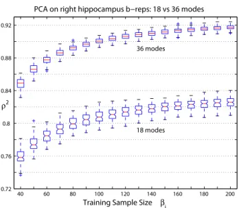
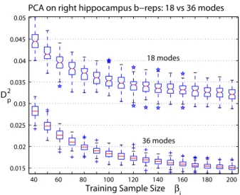
3.4.4 Experiments on Right Hippocampus B-reps . . . 68
3.5 Distance Measures for ρ2 Evaluation . . . 69
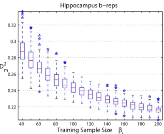
3.5.1 Application ofD∗2 to Right Hippocampus B-reps . . . 71
3.6 Goodness of Prediction ρ2dfor Curved Manifolds . . . 72
3.6.1 Two Possible Extensions ofρ2 . . . 72
3.6.2 ρ2d for Nonlinear Shape Models . . . 73
3.7 Application ofρ2d on Models in Nonlinear Space . . . 74
3.7.1 Deformed Binary Ellipsoids . . . 74
3.7.2 Experiment on M-rep Fits to Deformed Binary Ellipsoids . . . 75
3.7.3 Experiment on Right Hippocampus M-rep . . . 76
3.7.4 Evaluation of a Coarse-to-fine Shape Prior . . . 77
3.8 Conclusion & Discussion . . . 79
4 Multi-Object Statistical Shape Models2 . . . 82
4.1 M-rep Operations . . . 85
4.1.1 Residues of the Object Variations . . . 86
4.2 Inter-Object Relations . . . 87
4.2.1 Augmentation . . . 87
4.2.2 Prediction . . . 88
4.3 Propagation of Sympathetic Changes . . . 89
4.3.1 Residues of Objects in Order . . . 92
4.3.2 Training the Probability Distribution per Object . . . 92
4.3.3 Geometrically Proper Objects . . . 93
4.4 Decomposition of Shape Variations . . . 97
4.4.2 An Iterative Method . . . 99
4.4.3 Joint Probability of Multiple Objects . . . 101
4.4.4 Shape Prior in MAP-Based Segmentation . . . 102
4.4.5 Segmentation of Male-Pelvis Model . . . 103
4.4.5.1 Probability Density Estimation . . . 103
4.4.5.2 Segmentation Results . . . 105
4.5 Discussion and Conclusion . . . 108
5 Conditional Shape Statistics3 . . . 111
5.1 Conditional Probability Distribution . . . 112
5.2 Estimation of Conditional Shape Distribution using PCR . . . 113
5.3 Applications of CSPD to Deformable M-rep Segmentation . . . 115
5.3.1 Simulated Multi-objects . . . 115
5.3.1.1 Training Results . . . 117
5.3.2 Objects in the Pelvic Region of Male Patients . . . 119
5.3.2.1 Results of Within-patient Successive Segmentations . . . 120
5.4 Discussion and Conclusion . . . 123
6 Discussion and Conclusion . . . 125
6.1 Summary of Contributions . . . 125
6.2 Evaluation of Statistical Shape Models . . . 131
6.2.1 Discussion . . . 131
6.2.2 Future Work . . . 137
6.3 Multi-Object Statistical Shape Models . . . 137
6.3.1 Discussion and Future Work . . . 137
List of Tables
4.1 Total variations of self and neighbor effects per bladder, prostate, and rectum . 104
5.1 Number of fractions (sample size) per patient . . . 118
5.2 Mean volume overlaps of figure 5.3 . . . 121
List of Figures
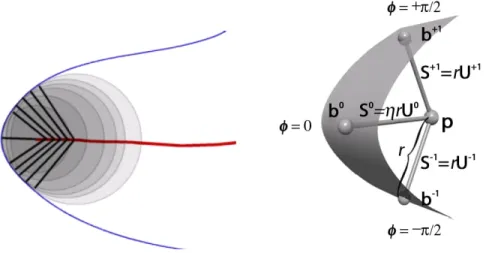
2.1 Different classes of medial points . . . 45
2.2 Medial geometry of end atoms . . . 47
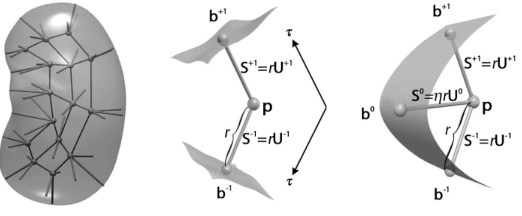
2.3 A discrete m-rep . . . 49
2.4 Segmented kidney m-reps . . . 54
3.1 Simulated deformed ellipsoids . . . 64
3.2 Two bar graphs of the first 10 eigenvalues in percentage estimated from 5000 simulated warped ellipsoids b-reps . . . 65
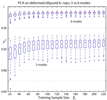
3.3 Box plots ofρ2 for PCA on warped ellipsoid b-reps . . . . 66
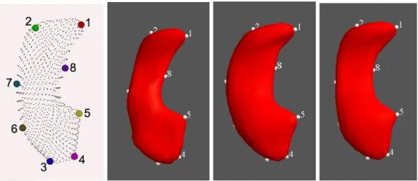
3.4 Landmarks of hippocampus and 3 fitted hippocampus m-reps . . . 67
3.5 Two bar graphs of the first40eigenvalues in percentage estimated from290right hippocampus b-reps. . . 68
3.6 Box plots ofρ2 for PCA on right hippocampus b-reps . . . 69
3.7 A box plot of D2 m estimated from right hippocampus b-reps . . . 71
3.8 Two box plots of D2 p for PCA on right hippocampus b-reps . . . 72
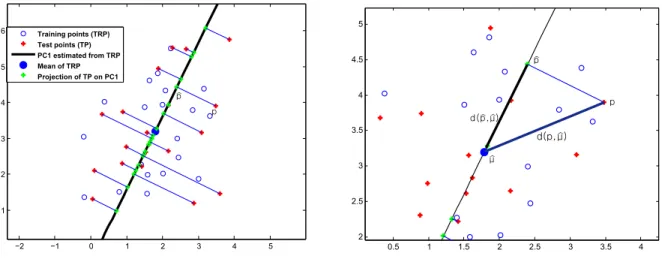
3.9 Graphical interpretation of ρ2 . . . 73
3.10 A(128×128×128) bent and tapered binary ellipsoid . . . 74
3.11 Two box plots ofρ2 d for PGA on m-rep fits to deformed binary ellipsoids . . . . 75
3.13 Four simulated ellipsoids with local deformation . . . 77
3.14 Two box plots of ρ2 d for multi-scale PGA on simulated ellipsoid m-reps with local deformation . . . 77
3.15 Two box plots ofρ2 d for multi-scale PGA on simulated hippocampus m-reps . . 79
4.1 An m-rep 3-object complex for the bladder, the prostate, and the rectum of a patient in different view. . . 84
4.2 Augmented atoms of the prostate and the bladder. . . 88
4.3 Illustration of the sympathetic change ofR01 caused by N1 . . . 90
4.4 Augmented atoms in the bladder and the prostate . . . 91
4.5 M-rep sampling . . . 94
4.6 Illustration of first modes of variation of two patients . . . 96
4.7 Predicted Prostates of a patient B163 . . . 100
4.8 A bladder and a prostate m-reps on the left and the predicted prostate shape caused by the changes in the bladder . . . 105
4.9 A log plot of total variances over 200 iterations . . . 106
4.10 Segmentation of the bladder and the prostate of patient 3106 and 3109 . . . 107
4.11 Segmentation of the prostate and the bladder of patient 3109 . . . 107
4.12 Plots of sorted volume overlaps and average distances of the prostate segmen-tations . . . 108
5.1 Simulated quasi-bladder, quasi-prostate, quasi-rectum complexes . . . 114
5.3 Plots of mean prostate volume overlaps and average surface distance in mm . . 119
5.4 Plots of segmented JSC and average surface distance in mm . . . 122
6.1 (a) Eigenvalue plots of PGAMR and PCASE of simulated ellipsoid m-reps. (b) Box plots ofρ2
d on the simulated ellipsoid m-reps and the derived b-reps. . . 132
6.2 (a) Eigenvalue plots of PGAMR and PCASE of deformed ellipsoid binaries. (b) Two box plots of D2
p on warped ellipsoid binaries. . . 133
6.3 (a) Eigenvalue plots of PCA on hippocampus b-reps and of PGA on the cor-responding hippocampus m-rep. (b) Two box plots of ρ2 on the hippocampus b-reps and m-reps. . . 133
6.4 Comparison of projections of 50 m-rep fits to deformed binary ellipsoids and of the corresponding 50 b-reps on each shape space . . . 135
Chapter 1
Introduction
1.1
Motivation
Medical imaging has developed rapidly for the last several decades. Physicians can see inside a human body without cutting the body open via medical imaging. Various imaging modalities have emerged such as magnetic resonance imaging (MRI), ultrasound imaging, x-ray com-puted tomography (CT) and functional magnetic resonance imaging (fMRI). These imaging techniques produce high-resolution images of different properties of a human body that the naked human eye cannot perceive. The goal of medical image analysis is to make the best use of the information contained in these images. To that end it provides advanced tools that can help to improve diagnosis of disease, to understand the physiology of a human body, or to plan therapy such as radiation treatment.
probability distribution of the geometric shape variation of organs observed in training data. Another application of statistical shape analysis can be found in the study of mental illnesses such as autism and schizophrenia. These illnesses have been reported to affect the shape of some brain structures as the illnesses progress. In the brain of schizophrenics, shapes of some parts of the hippocampus are different from those of non-schizophrenics. With brain structures extracted from the images, statistical shape analysis on their shapes and the inter-relation between structures can aid the understanding of the illnesses by providing a means to compare the shapes of brain structures between the ill and the healthy. It can ultimately serve clinicians as a diagnostic tool for early detection of such illnesses.
Statistical shape analysis hinges on the geometric representation of objects. The repre-sentation needs to capture the geometric properties and be consistent across all instances of the object of interest in describing the structure and features of the object. Many efforts have been made to find an appropriate geometric representation of either 2D or 3D objects. Among various models that have been actively investigated, some of the well-known ones are the following: active contour models [Malladi et al., 1995a] and its variant geodesic active contour models [Caselles et al., 1995], diffeomorphisms from atlases [Joshi, 1997, Christensen et al., 1997], level set models [Malladi et al., 1995b, Tsai et al., 2003], point distribution models (PDM) [Cootes et al., 1995] and m-reps [Pizer et al., 2003]. Most shape models of an object are based on a representation of the boundary that lives in a vector space; in that case the shape variations of the object are captured by changes in the boundary. In contrast, the m-rep is derived from a medial representation that focuses on representing the interior of an ob-ject. The m-rep describes local shape changes of an object uniquely by thickening, elongation, bending, and twisting.
information on the variation of the object unless the variation of its neighboring objects is considered together. A shape probability distribution that properly includes the information of its neighboring objects can play a crucial part in identifying the target object in a new image, especially when the boundaries of objects are so indistinct that even clinicians have difficulty in identifying a target object among its neighboring objects.
This dissertation develops novel alternative techniques to estimate a shape probability distribution of multi-object complexes. A new aspect of this work is to include in a shape probability distribution the relation of neighboring objects to the target object by means of augmentation, that is, augmenting features of its neighboring objects that are highly correlated with the target object to features of the target object. This work consists of two parts. The first one is a method to estimate a conditional shape probability distribution of a target object given its neighboring objects. This method is based on principal component regression (PCR) [Shawe-Taylor and Cristianini, 2004] in reflecting the effect of neighboring objects on the target object. PCR corresponds to performing principal component analysis and regressing in the feature space given by the few first principal directions that capture major variations explained in a given sample. The second part is an approach to estimate shape variation of each object in a grouped multi-object complex where each object’s variation is considered to have two components: one being the object’s variation independent of its neighbors’s effect and the other being the object’s interaction with its neighbors. This explicit separation of shape variation into two components is based on the concept of residue introduced in [Lu et al., 2007] for multi-scale shape analysis.
In the study, goodness of prediction is analyzed as a function of training sample size. This approach of analyzing the correlation measure with respect to sample size enables us not only to deduce the statistical properties of the stability but also to determine an approximate minimum sample size that guarantees a given extent of predictive power. This approach also addresses the issue of sample size that arises in estimating statistics of shape descriptions.
Most statistical shape analysis methods suffer from small sample size. Available training samples are limited due to the cost and time involved in the manual segmentation of medical images. In addition, the dimension of shape feature spaces is in general very high, about several hundreds or thousands, due to the complexity of shape of objects in medical images. Samples of an object’s shape in most shape representations are thus typical high dimensional low sample size (HDLSS) data sets. That is, the dimension of the data features is much larger than the sample size. This HDLSS nature of shape data presents a challenge because estimation of shape probability distributions can be very unstable as training samples from the population change. Moreover, many classical data analysis methods in statistics cannot be blindly applied to HDLSS data.
It is hard to avoid the HDLSS problem in statistical shape analysis. In such a situation, a method that can decide the minimum size of training sample that ensures some degree of predictive power holds practical importance, especially to applications of statistical shape analysis. To my knowledge, this is the first work to present an evaluation method of estimated shape probability distributions that has the capability to indicate the predictive power of the estimated distribution at a given sample size.
This dissertation focuses on estimation of shape probability distribution of multiple objects and evaluation of the estimated shape probability distribution. The following subsections describe more in detail the driving problems, challenges, and scopes of two main topics in this dissertation.
1.1.1 Statistical Shape Analysis of Multiple Objects
anal-ysis of multi-object complexes can be classified in terms of object features as follows: 1) by object complex, 2) object by object, 3) hierarchically from the object complex to the individual objects. The object complex approach has been applied to many current shape models since it is simple and straightforward. This global approach fails to capture the local variation of an object itself and sometimes gives misleading information about the inter-relation among objects because information at global and local scales are mixed in the features.
The object-by-object approach may capture sufficient information about the variability of each object’s shape itself in an estimated shape probability distribution. However, the shape probability distribution of an object itself does not have explicit knowledge about the interaction among objects, so it cannot be used to infer the interaction.
The hierarchical approach addresses the issue of scales in shape models. It computes multi-object shape statistics from the scale of an multi-object complex down to the level of individual objects [Kapur et al., 1998, Vaillant and Davatizikos, 1999]. [Davatzikos et al., 2003] even consider the residue from a larger scale successively. The problem in the hierarchical approach is that it is difficult to come up with a reasonable criterion to define what the variations in object-complex scale and in object-itself scale are, and to distinguish one from the other. The weaknesses in these approaches suggest that we need to somehow reflect the effects from neighboring objects in describing the variation of each object in the object complex.
multi-object complex especially when organs are clumped together and touch each other and when the low physical contrast in the image between such structures makes significant parts of the boundary of the target organ ambiguous.
My approach to estimation of the conditional shape distribution is based on the principal components regression (PCR) method [Shawe-Taylor and Cristianini, 2004]. Estimating both the conditional mean and the shape distribution involves computing an inverse of a sample covariance matrix. The limited sample size and high dimensional feature space of shape de-scriptors provides a challenge in computing an appropriate pseudo-inverse of the covariance matrix. As described before, PCR is equal to regressing in the feature space given by the major principal directions that PCA on the input data produces. Using PCR in reflecting the effect of neighboring objects on the target object in the conditional term of the conditional probability distribution has the following advantages. First, doing PCA on the neighboring shape features reduces the dimension of the feature shape space of neighbor objects. In the reduced features shape space, it is possible to compute a non-singular sample covariance ma-trix and get a stable estimate of its inverse. Second, it can help to tighten the distribution of the estimated conditional probability distribution since major variation of the neighboring objects is explained in the reduced feature space.
The second approach to shape analysis of multi-object complexes is to divide shape vari-ation of each object in grouped multiple objects into two components: one being the object’s inherent shape variation and the other being the object’s shape change caused by the interac-tion with its neighbors, which must sum to the overall shape variainterac-tion of each object. Thus, one component must be regarded as the residue of the other from the total variation of an object observed.
probability distribution of each object. Since both approaches estimate the shape probability distribution object-by-object, the HDLSS problem does not get worse as it would in the global approach. [Lu et al., 2007] provides a detailed explanation about the advantages in considering various degrees of locality in the shape variation of an object and in describing an object’s variation via the residue within and between scales.
1.1.2 Quality Measures of Statistical Shape Models
Due to the variety of statistical shape models, one can desire some criteria to evaluate a statistical shape model for its effectiveness and some procedures to compare different statistical shape models so as to help choosing an appropriate one that meets one’s need. Many models for single objects are already available to geometrically represent shape and to statistically analyze geometric representations. In addition, new models for multi-object complexes are emerging, as mentioned in the previous section.
shape can help to alleviate the HDLSS problem as well as to avoid the over-fitting problem. Third, an estimated shape probability distribution needs to be tight. Fourth, it needs to be unimodal since most statistical data analysis methods employed in shape analysis are based on the assumption of Gaussian distribution of the data. Fifth, a statistical shape model must be able to represent only real instances in the population of the geometric entity. Sixth, it must be able to describe a member of the population unseen in a training sample.
Among the few studies in which statistical shape models were evaluated, a key study done by Styner et al. [2003] defines three criteria that can assess some of these properties and then compares correspondence of shape models on the basis of the three criteria. The three criteria are defined as follows: compactness as the ability to use a minimal set of parameters, gener-alization as the ability to describe instances outside of the training set, and specificity as the ability to represent only valid instances of the object in its population. Generalization ability is assessed by doing leave-one-out reconstruction and computing approximation errors of un-seen models averaged over the complete set of trials. These measures are defined as functions of the number of shape parameters. Generalization ability and specificity are defined in the
ambient space, where the models lie physically. In regard to these criteria, Styner et al. [2003] examined and compared four methods: a manually initialized subdivision surface method for direct correspondence and three automatic methods - spherical harmonics, minimum descrip-tion length, and minimum covariance determinant - for model-implied correspondence across instances of an object.
While these measures offer legitimate criteria to evaluate correspondence methods of dif-ferent statistical shape models, they are short on the predictive power of the statistical shape models: the ability to describe unseen members of the population and to describe their fre-quency of occurrence. This ability of statistical shape models is critical since most applications of statistical shape models heavily rely on their predictive power. One example is model-based segmentation in the maximum a posteriori (MAP) framework, which uses a prior distribution of shape of an geometric entity to extract the geometric entity from a new image. Another example is classification of an object on the basis of its shape, using trained shape prior distributions.
Muller [2007] proposed a novel statistical correlation measure that evaluates the predictive power of statistical shape models derived using principal component analysis (PCA). Muller first shows that PCA can be recast as a multivariate regression model by treating the observed variables as responses and principal directions as predictors. Then, goodness of prediction is derived from goodness of fit, a standard statistical measure for second moment accuracy. As for possible goodness of prediction measures, he proves that canonical correlations and related measures of association degenerate to constants and that the “univariate approach to repeated measures” test (average squared correlation, generalized variance explained) provides a simple and useful measure of association. He also suggests another measure - squared multiple correlation - to provide more detailed information. Among the several measures he proposes, in this work we adopt the average squared correlation measure as a goodness of prediction measure to evaluate the predictive power of both linear and nonlinear statistical shape models. The detailed development of this measure is given in chapter 3.
This correlation measure has a clear statistical interpretation in terms of the predictability of statistical shape models. This feature facilitates evaluation and comparison of different approaches to estimate a shape description or different statistical shape models. Furthermore, the average squared correlation is a simple direct measure defined in the shape feature space and is quick and easy to compute. In contrast, the generalization measure in [Styner et al., 2003] is an indirect measure defined in the ambient space where the models lie physically, and it takes a long time to compute.
the predictive power of statistical shape models as a function of training sample size using goodness of prediction. This correlation measure is first extended to nonlinear manifolds as some shape representations like the m-rep do not belong to a vector space. This work then demonstrates the procedure with two different shape representations: the m-rep and the PDM. The PDM is a well-known and popular shape model that represents an object by concate-nated points sampled on the surface of an object. In training its shape probability distribution, PCA is applied to reduce the dimension of the representation as well as to find modes of varia-tion that are significant in the training sample. The m-rep on the other hand takes the object interior into account, and the boundary of the object is derived indirectly from the represen-tation. Unlike the PDM, the m-rep does not lie in Euclidean space because of the radius and the rotational components of the medial atoms. Fletcher et al. [2004] found that an m-rep can be understood as a point in so called “symmetric space” where the properties of vector space do not hold. They developed principal geodesic analysis (PGA) that generalized PCA in the abstract, curved space known as manifolds. Due to their distinctive contrast in their perspectives to describe an object, the PDM with PCA and the m-rep with PGA are chosen for this work.
1.2
Thesis
Thesis: (1) Reflecting interaction among objects in statistical shape models for multi-object complexes via augmentation yields a shape probability distribution that can capture the
config-uration of objects and shape variability caused by neighboring objects.
(2)A systematic procedure to evaluate the predictive power of statistical shape models as a function of training sample size using the correlation measure provides a means to determine
an approximate minimum size of sample that ensures a certain degree of predictive power and
stability.
1.3
Claims
The contributions of this dissertation are as follows:
1. It is shown that in multi-object statistical shape analysis augmentation of highly corre-lated geometric features of neighboring objects to the target object can be used to reflect interaction among objects in shape probability distribution of the target object.
2. A new method to estimate the shape probability distribution of an object conditioned on its geometric primitives of the neighboring objects has been developed. The method relies on principal component regression to have stable and reliable estimates of the conditional mean and the conditional covariance matrix.
3. The conditional shape probability distribution can usefully provide a shape prior for max-imum posterior segmentation with the conditional mean as the initial template model. This conditional shape prior was applied to segment anatomical objects in the male pelvis.
4. A method to decompose shape variation of each object in multi-object complexes into two components has been developed on the basis of the concept of the residue.
segmen-tation. These shape priors of the decomposed shape variations were applied to segment anatomical objects in the male pelvis.
6. A new correlation measure called goodness of prediction initially proposed by Muller [2007] in linear space has been extended to shape representations that live in a nonlinear manifold.
7. As a tool to evaluate the predictive power of statistical shape models, an iterative pro-cedure that estimates the goodness of prediction in a given set of samples has been developed. This procedure provides a means to analyze the correlation measure for a given statistical shape model as a function of training sample size.
1.4
Overview of Chapters
Chapter 2
Background
This chapter presents the background material from statistics and image analysis that is rele-vant to this dissertation. Section 2.1 gives an overview of basic concepts of probabilities and statistical methods that are central to this dissertation. Section 2.2 explains the statistical the-ory of shape, which lays the background for the next section. Section 2.3 explains probabilistic deformable models and a few geometric representations of objects. Then, section 2.4 describes in detail the medial object representation, a deformable model used in this dissertation. Sec-tion 2.5 describes transforming human expert segmentaSec-tions into models that will be used to learn the probability distribution on the anatomic shape of interest. The last section: 2.6 explains the segmentation of m-reps.
2.1
Statistical Background
2.1.1 Probability Distributions
This section starts from the basic definitions of probability, random variables, probability distributions and elementary statistics, and it ends with the well-known multivariate normal distribution that appears repeatedly in this dissertation. Most materials in this section are from [Hogg and Craig, 1995, Muirhead, 1982].
2.1.1.1 Definitions
on subsets of the space C such that [Hogg and Craig, 1995]
(a) P(C)≥0,
(b) P(C1∪C2∪. . .) =P(C1) +P(C2) +. . ., where the sets Ci, i= 1,2,3, . . . ,are such that
no two have a point in common (that is, whereCi∩Cj =∅, i6=j), and
(c) P(C) = 1.
The probability functionP(C) tells us how the probability is distributed over various subsets
C of the sample space C.
In some experiments we are concerned only with outcomes that are elements of a subset
C1 of the sample space C. The sample space then becomes in effect the subset C1. For C2
another subset of C, the conditional probability P(C2|C1) of the event C2 given the eventC1
is defined as
P(C2|C1) =
P(C1∩C2)
P(C1)
, (2.1)
provided that P(C1) > 0. That is, P(C2|C1) considers only those outcomes in C2 that are
elements of C1. P(C2|C1) also has the following properties:
1. P(C2|C1)≥0,
2. P(C2∪C3∪. . .|C1) =P(C2|C1) +P(C3|C1) +. . ., whenC2, C3, . . .are mutually disjoint
sets, and
3. P(C1|C1) = 1.
These are the precise conditions that a probability function must satisfy as described above. Occasionally, the occurrence of an event C1 does not change the probability of an event C2,
i.e.,
P(C2|C1) =P(C2).
In this case, the eventsC1andC2 are said to beindependent. From the definition of conditional
probability, we can see that two independent events satisfy
which can be used as an alternative definition of independence.
The famous Bayes’ rule is also derived from the definition of conditional probability. The conditional probability of the eventC1 given the event C2 is
P(C1|C2) =
P(C1∩C2)
P(C2)
. (2.2)
SinceP(C1∩C2) is the common term both in (2.1) and (2.2), (2.1) and (2.2) can be rearranged
and combined to obtain Bayes’ rule:
P(C1|C2) =
P(C1∩C2)
P(C2)
= P(C2|C1)P(C1)
P(C2)
, (2.3)
which relates two conditional andmarginal probabilities of the events C1 and C2. The
defini-tion of a marginal probability will be given later in secdefini-tion 2.1.1.5.
Arandom variable X is a function that assigns to each elementc∈ C one and only one real number X(c) =x. The space of X is the set of real numbers A={x∈R:x=X(c), c∈ C}. Thus, a random variable X is a function that carries the probability from a sample spaceC to a spaceAof real numbers. The probabilityP(A) now defined onA,A⊂ A. Ais also referred to as the sample space.
If A contains a finite number of points or the points of A can be put into a one-to-one correspondence with the positive integers, X is called a random variable of the discrete type. If the random sample spaceAconsists of an interval or a union of intervals in R,X is said to
be a random variable of the continuous type. This work deals with only random variables of the continuous type, so topics about discrete random variables will be not be discussed here. Random variables will refer to continuous random variables from now on.
The probability P(A), A ⊂ A can be expressed in terms of a nonnegative function f(x) such that
Z
A
f(x)dx= 1,
by
P(A) =
Z
A
f(x)dx.
f(x) is called the probability density function (p.d.f.) of X. When A is an unbounded set from−∞to a real number x, the distribution function (or sometimes,cumulative distribution function) F(x) =P(X ≤x) is defined as
F(x) =
Z
w≤x
f(w)dw.
2.1.1.2 Expectations of a Random Variable
Let X be a random variable having a p.d.f. f(x). A central value of the probability is given by the expectation of the random variable X:
E(X) =
Z ∞
−∞
xf(x)dx.
For example, the expectation of the random variable X = ln (r) gives the central value of ln (r) when its p.d.f. is known. For a function of X, Y =u(X), the expectation of u(X) is
E(u(X)) = R∞
−∞u(x)f(x)dx. When u(X) = X, E(X) is the arithmetic mean of the value of X, and is called the mean value of X. Another special expectation is obtained by taking
u(X) = (X−E(X))2, that is,
E(X) =
Z
x
(x−E(X))2f(x)
2.1.1.3 Special Distributions
Two important distributions are introduced in this section. They are frequently used in statis-tics and mentioned in this dissertation.
The Normal Distribution
A random variable X that has a p.d.f. of the form
f(x) = 1
σ√2π exp
−(x−µ)
2
2π2
, −∞< x <∞ (2.4)
is said to have a normal orGaussian distribution with mean µand variance σ2. The normal p.d.f. occurs so often in many parts of statistics that it is denotedN(µ, σ2). A useful property of the normal p.d.f is that given a random variable X that is N(µ, σ2), the random variable
W = (X−µ)/σ is N(0,1). This fact helps with simplifying the calculations of probabilities concerning normally distributed random variables.
The log of the scale component ln (r) in m-reps is assumed to follow the normal distribution, i.e., ln (r) ∼ N(0, σ2) of mean zero and a standard deviation σ, when treated as a random variable in shape analysis of m-reps.
The Gamma and Chi-Square Distributions
A random variable X that has a p.d.f
f(x) = 1 Γ(α)βαx
α−1exp(−x/β), 0< x <∞
= 0 elsewhere
is said to have a gamma distribution with parameters α and β. The gamma function of α is defined as Γ(α) =R0∞yα−1exp(−y)dy, which exists for α >0. The value of the integral is a positive number. Achi-square distribution is a special case of the gamma distribution in which
α =γ/2, where γ is a positive integer, and β = 2. The parameter γ is called the number of degrees of freedom of the chi-square distribution. X is χ2(γ), i.e.,X ∼χ2(γ) means that the random variableX follows a chi-square distribution withγ degrees of freedom.
N(µ, σ2). So the square of the log of the spoke length components in m-reps (ln (r)/σ)2 is also χ2(1).
2.1.1.4 Statistics: Sample Mean and Variance
A statistic is a function of one or more random variables that does not depend on any un-known parameters although the distribution of the statistic may depend upon the unun-known parameters. Let the random variables Xi, i= 1, . . . n, be independent, each having the same
p.d.f f(x). For example, if X1 isN(µ, σ2), then a random variableY = (X1−µ)/σ isN(0,1)
and is a function ofX1 that depends on the two parametersµand σ, so it is not a statistic. In
contrast, Y =Pn
i=1Xi does not depend on any unknown parameters and thus is a statistic.
A statistic can be used to infer information about the unknown parameters. Let a random variableX be defined on a sample spaceA. In many situations, the distribution ofXis known except for the value of the parameters of the distribution. To obtain information about the unknown parameters, the random experiment is repeatednindependent times under identical conditions. If the random variable Xi is a function of the i-th outcome, i = 1, . . . , n, then
X1, X2, . . . , Xn are called the observations of a random sample from the distribution under
consideration. If we have a statistic Y = u(X1, . . . , Xn) whose p.d.f is known and the p.d.f
reaches its maximum when Y has a value close to the unknown parameter, then the statistic
Y can be used to draw information about the unknown parameters.
The most common statistics are the mean and the variance of the random sample. Let
X1, X2, . . . , Xndenote a random sample of size n from a given distribution. The mean of the
random sample is defined as
b
µ= X1+. . .+Xn
n = n X i=1 Xi n .
The variance of the random sample is defined as
b
σ2 =
n
X
i=1
(Xi−µb)
2
n−1 =
n
X
i=1
Xi2 n−1 −
n n−1bµ
2.1.1.5 Multivariate Distributions
Describing shapes of objects in 2D or 3D usually requires multiple features, such as the ordered tuple of points on the surface, a set of control points of spline functions that represent the surface, or a set of curvatures. Statistical shape analysis considers these geometric features as random variables and focuses on understanding their relation, variability and geometrical properties. The analysis of more than one variable requires multivariate statistics.
Let Xi,i= 1, . . . , p be a set of random variables. The space of these random variables is
the set of ordered p-tuples A = {(x1, . . . , xp) : x1 = X1(c), . . . , xp = Xp(c), c ∈ C} where C
is the sample space. For A⊂ A the probability function of these p-variate random variables
P(A) can be expressed as
P(A) =
Z
· · ·
Z
A
f(x1, . . . , xp)dx1. . . dxp.
In parallel to the definition of a p.d.f for a single random variable, f is a p.d.f iff is defined and is nonnegative for all values in A, and if its integral over all real values in A is 1. The distribution function of Xi,i= 1, . . . , pis
F(x1, . . . , xp) =P(X1 ≤x1, . . . , Xp≤xp)
If X1, . . . , Xp are continuous type random variables, f1(x1) is called the marginal p.d.f of X1
when
f1(x1) =
Z ∞
−∞ · · ·
Z ∞
−∞
f(x1, x2, . . . , xp)dx2. . . dxp.
The marginal probability density functionsf2(x2), . . . , fp(xp) forX2, . . . , Xp are defined
simi-larly as (p−1)-fold integrals. The marginal p.d.f can be generalized to a joint marginal p.d.f for any k < pgroup of random variables.
the vectorx is defined to be the vector of expectations:
E(x) =
E(X1)
.. .
E(Xp)
.
When dealing with ap-variate random vectorx∈Rp with meanE(x) =µ, the variance is defined by a covariance matrix. The covariance matrix ofxis defined to be the p×p matrix
Σ =Cov(x) =E[(x−µ)(x−µ)0].
The i,jth element of Σ is
σij =E[(Xi−µi)(Xj−µj)],
and theith diagonal element is
σii=E[(Xi−µi)2].
Clearly, Σ is symmetric, i.e., σij = σji. It is also a non-negative definite matrix. A p×p
symmetric matrix A is called non-negative definite if
α0Σα≥0 for all α∈Rp
and positive definite if
α0Σα >0 for all α ∈Rp, α6=0.
2.1.1.6 The Multivariate Normal Distribution
The p×1 random vectorx is said to have ap-variate normal orGaussian distribution if, for every α ∈Rp, the distribution of α0x is univariate normal (2.4) [Muirhead, 1982]. From this definition it can be shown thatx has the following density function [Arnold, 1981]:
f(x) = 1
(2π)p/2det(Σ)1/2exp − 1
2(x−µ)
0Σ−1(x−µ)
whereµ and Σ are the mean and the covariance matrix ofx respectively. det(Σ) denotes the determinant of the covariance matrix Σ. The p-variate normal distribution ofxis denoted by
Np(µ,Σ).
A multivariate normal random vectorxhas important properties as to the marginal distri-butions and the relation between its subvectors. These properties play an important part in the method developed in chapter 5 for multi-object shape analysis. If xisNp(µ,Σ), the marginal
distribution of any subvector of k elements of xis k-variate normal (k≤p). Moreover, x,µ, and Σ can be partitioned as
x= x1 x2
, µ=
µ1 µ2
, Σ =
Σ11 Σ12
Σ21 Σ22
,
where x1 and µ1 are k×1 and Σ11 is k×k. The subvectors x1 and x2 are independent if
and only if Σ12 = 0. In order to determine the independence of two subvectors of a normally
distributed vector, it suffices to check that the covariance matrix of the two subvectors is zero. Let Σ11·2 be Σ11 − Σ12Σ22−Σ21, where Σ−22 indicates a generalized inverse of Σ22, i.e.,
Σ22Σ−22Σ22= Σ22. Then
(a) x1−Σ12Σ−22x2 isNk(µ1−Σ12Σ−22µ2,Σ11·2) and is independent ofx2, and
(b) the conditional distribution of x2 given x1 isNk(µ1+ Σ12Σ−22(x2−µ2),Σ11·2) .
Item b implies that the covariance matrix Σ11·2 of the conditional distribution ofx1 given x2
does not depend onx2. The independence property of Σ11·2 on x2 comes in useful later when
the conditional distribution is used to estimate a multi-object shape probability distribution. Also, the mean of the conditional distribution of x1 given x2 is
E(x1|x2) =µ1+ Σ12Σ−22(x2−µ2).
E(x1|x2) is called the regression function ofx1 onx2 with theregression coefficients Σ12Σ−22.
It is a linear regression function since it depends linearly on the variablesx2 [Muirhead, 1982].
independent coordinates. Let ΥΛΥ0 be the eigendecomposition of Σ, where Λ is a diagonal matrix andΥis an orthonormal matrix whose columns are the new coordinate axes. In fact,
Υis a rotation matrix inSO(p). The covariance of the rotated vector ofx, namely,y=Υx, is
Σy=E[(y−µy)(y−µy)0]
=E[(Υx−Υµ)(Υx−Υµ)0] =E[Υ(x−µ)(x−µ)0Υ0] =ΥΣΥ0=Λ,
which shows that the random variables in the random vector yare independent.
2.1.2 Principal Component Analysis
Principal component analysis (PCA) is a technique developed by Hotelling [1933] to reduce the dimension of feature space without losing too much of the information about the variables contained in the covariance matrix. In most practical situations it is useful to describe a simple model for the structure of the corresponding covariance or correlation matrix for observations made on a large number of correlated random variables. In PCA, the original coordinate axes (variables) are rotated to give a new coordinate system having some optimal variance properties. The first principal component (variable) is the linear combination of the original variables with maximum variance; the second principal component is the linear combination of the variables having maximum variance uncorrelated with the first principal component; and so on. Thus, PCA attempts to find a new set of variables that can express larger variance with fewer variables.
There is a family of probability distributions called elliptical distributions. Elliptical dis-tributions are unimodal and symmetric around the mean. It follows that the contours of equal probability density form ellipsoids. The principal components of such a distribution describe a rotation of the coordinate axes to the principal axes orprincipal directions (vectors) of the ellipsoid. [Muirhead, 1982]
forms an elliptical distribution. If random variables of feature space are considered to follow a multivariate normal distributions, the principal directions of observations taken on the random variables and their corresponding variances give a way to find these contours of equal probabil-ity along each principal direction, which can be interpreted as fitting a Gaussian distribution. PCA can also be considered as a special case of a factor analysis (FA) in the context of
linear models. Factor analysis is a method to uncover the latent structure (dimensions) of a set of observed variables and thus to reduce the attribute space from a larger number of variables to a smaller number of so calledfactors. [Tucker and R., 1993] The FA model is often preferred over the PCA model because the PCA model underfits when the FA model holds. The underfitting always leads to bias and an invalid model, no matter how large the sample size is [Muller and Stewart, 2006]. PCA is also sensitive to the choice of a particular coordinate system or units of measurements of the variables because the method is not invariant under linear transformations of the variables so a linear transformation changes the eigenstructure of the covariance matrix [Muirhead, 1982]. In spite of these drawbacks of PCA, in medical image analysis PCA has proven its usefulness for describing the variability of linear shape data as shown in the early work of Cootes et al. [1995], Bookstein [1999].
The usefulness of PCA in shape analysis is twofold: (1) producing linear combinations of shape feature variables that give an efficient reparametrization of the original shape feature variables by the variability observed on the training data and (2) reducing the dimension of the original feature space into a subspace, a statistical shape space that is described by the estimated principal directions of major variances.
The objective of PCA is to find a subspace centered at the mean that best explains the variability observed in the data. PCA can be formulated in two ways (1) an approach to minimize the sum-of-squares of the residuals to the data and (2) an approach to maximize the total variance of the projected data. Jolliffe [1986] shows that both approaches produce the same subspace in linear space. A concise summary of both approaches is given in [Fletcher, 2004]. Here only the second approach is described.
data with their meanµ. The total variance is defined as
σ2 = 1
N
N
X
i=1
kyi−µk2=
1
N
N
X
i=1
hyi−µ,yi−µi2. (2.5)
Principal directions, ormodes of variationvj, spanning thek-dimensional linear subspace Vk,
j= 1. . . k and k≤p, are given by
vj = argmax kvk2=1
N
X
i=1
hyij,vi2 , (2.6)
whereyij,i= 1, . . . , N, satisfies the recurrence relation:
y1i =yi−µ
yij =yji−1− hyij−1,vj−1ivj−1 .
That is, yji are the points of yi−µ projected on to the subspace orthogonal to Vj−1. These
principal directions vi define a subspace that maximizes the total variance of the projected
points. Principal components are the projection coefficients of the multivariate data y ∈Rp
onto the principal directions, i.e.,hy−µ,vji.
PCA in Matrix Notation
PCA can also be understood as a way to decompose the sample covariance matrixS of the
yi’s. LetY be a N ×p data matrix where each row isyi0, that is,
Y=
y01
.. .
y0N
.
Letµb be the p×1 sample mean vector of Y. µb can be written in matrix notation as
b µ= 1
N
N
X
i=1
yi=
1
NY
where1 is the N×1 vector of 1’s. Thep×p sample covariance matrixS can be written as
S= 1
N −1
N
X
i=1
(yi−µb) (yi−µb)
0
= N
N −1
1
NY
0Y−
b µµb0
. (2.8)
Recall that the covariance matrix is symmetric (S = S0) and non-negative definite, which guarantees that its spectral decomposition or eigendecomposition produces only real and non-negative eigenvaluesλ1, . . . , λp, withλ1 ≥λ2. . .≥λp, and corresponding ordered eigenvectors
v1, . . . ,vp. This eigendecomposition ofS can be written as
Υ0SΥ= D (λ) ,
where
D (λ) =
λ1 · · · 0
..
. . .. ... 0 · · · λp
,
thep×p diagonal matrix of the eigenvalues{λi},i= 1. . . p, and where
Υ=
v1. . .vp
,
the column matrix of eigenvectorsv1, . . . ,vp. These eigenvectors are equivalent to the principal
directions defined in (2.6) defining a new set of coordinate axes. λ1, . . . , λp are estimates of
the variances of the population principal components of the population covariance matrix Σ.
Dimension Reduction and Approximation of Data
The estimated total variability or variance in Y is defined as
tr (S) = tr (D (λ)) =
p
X
i=1
λi ,
the trace of the sample covariance matrix S. This definition of total variance is equivalent to the previous definition in (2.5).
that, for example, explains a maximal percentage of the total variance. Projecting the data into the subspace Vpa spanned by the first pa principal directions allows us to approximate
the original y by the linear combination of the first pa principal directions weighted by their
corresponding principal components. The projectionya is then
ya=µb+
pa X
i=1
αivi , (2.9)
whereαi=hy−µb,vii fori= 1. . . p. These αi’s are the principal components.
As an aside, det(S) can be another measure of total variability. However, det(S) is not as popular as tr(S) since it is very sensitive to any small eigenvalues (variances) even though the others may be large. In PCA the hope is that for some smallpa,λ1+. . .+λpa is close to tr(S)
so the first pa principal components explain most of the variation in Y and the remaining
principal components contribute little. Section 3.1.2 of chapter 3 revisits the approximation of the shape data by estimated principal components.
PCA can be recast as the multivariate linear model by treating the observed variables as
responses and principal directions as predictors [Muller, 2007]. One major contribution in this dissertation is the introduction of a formal correlation measure called goodness of prediction described in chapter 3. The correlation measure is designed to evaluate statistical shape models that use principal component analysis (PCA) to characterize shape variability, in terms of their predictive power. This alternative interpretation of PCA as the multivariate linear model is a critical step in presenting the correlation measure. Another contribution on the analysis of object-relation in a multi-object complex is also based on a multivariate linear regression method modified by PCA. Therefore, the next section briefly touches on the multivariate linear model.
2.1.3 The Multivariate Linear Model
multivariate analysis.
The multivariate linear model allows two or more responses to be measured on each inde-pendent sampling unit. The definition given in [Muller and Stewart, 2006] is as follows.
Definition 1. A general linear multivariate modelY =XB+E with primary parametersB,
Σ(B is called the regression coefficient) has the following assumptions:
1. The rows of the N×prandom matrix Y correspond to independent sampling units, that is,Yi, i= 1, . . . , N are mutually independent where Yi is the ith row of the matrix Y.
2. The N ×q design matrix X has rank(X) =r ≤q ≤N and is fixed and known without appreciable error, conditional on knowing the sampling units, for data analysis.
3. The q×p parameter matrix B is fixed and unknown.
4. The mean of Y isµY =XB.
5. The mean of E is µE =0.
6. The rows of the response matrix Y has finite covariance matrix Σ, which is fixed,
un-known, and positive definite or positive semidefinite.
Each Yi, i = 1, . . . , N, is assumed to follow a multivariate normal distribution with the
same covariance matrix Σ. Then the maximum likelihood estimates of B and of Σare given as
b
B= X0X−1X0µbY = X
0
X−1X0Y,
and
b
Σ= 1
N(Y−XBb)
0(Y−X
b
B),
ifN ≥q+p.
2.1.3.1 Principal Component Regression
directions instead of the original features. Principal components that PCA produces from the input data becomes the new input data, which allows the dimension reduction and associated stability of the features in the input data. Shape analysis of multi-object complexes described in chapter 5 makes use of PCR in estimating a conditional covariance matrix of a target object given selected features in its neighboring objects of the multi-object complex. As can be seen in the equation of Σ11·2 in section 2.1.1.6 the estimation of the conditional covariance matrix
involves computing an inverse covariance matrix. PCA on the selected features in the neigh-boring objects reduces the dimension of the shape features and allows the stable estimation of the inverse covariance matrix.
Following the notation in definition 1, let X be a data matrix in which each row is an input data sample feature vector (independent variables, predictors) and Y be the desired output (dependent variables, responses) matrix. General linear multivariate regression can be considered as the optimization problem of the least squares equation
b
B= argmin
B
kXB−Y k2, (2.10)
whereBis theq×pregression coefficient matrix and the norm is taken as theFrobenius matrix norm, i.e., the sum of the squared norms of the individual errors.
Bysingular value decomposition (SVD) or PCA,X0 can be factored into a diagonal matrix
Λbetween two orthogonal matricesΥand V, i.e.,X0=ΥΛV0, whereΥisq×q,Λisq×N, andV isN×N. Λhas nonnegative numbers on the diagonal and zeros off the diagonal. The columns of Υare the principal directions (eigenvectors). Let Υk be the first k ≤q columns
of the matrix Υ and Λk be the k×N diagonal matrix of the first k rows of Λ. PCR takes
the first keigenvectors of X0X as the features while leavingY unchanged. That is, the data matrix now becomesXΥk and then the least squares equation (2.10) for PCR becomes
min
B kXΥkB−Yk
2 , (2.11)
orthogonal matrices. Since the norm does not change by pre-multiplication of an orthogonal matrix, (2.11) can be reduced as follows:
min
B kXΥkB−Yk
2 = min
B kV
0(XΥ
kB−Y)k2
= min
B kV
0
(VΛ0Υ0ΥkB−Y)k2
= min
B kΛ
0Υ0Υ
kB−V0Y k2
= min
B kΛ
0
kB−V 0Yk2 .
The solution ofB with minimal Frobenius norm is now simply
b
B = (ΛkΛ0k)−1Λ−k1V 0Y
= Λ−k1V0Y, (2.12)
where Λ−k1 is a k×N matrix whose diagonal elements are the reciprocals of the diagonal elements of Λk.
2.2
The Statistical Theory of Shape
In the past, image analysis has been focused on modeling and analysis of local features such as edges and colors at the pixel or voxel scale to characterize complex objects in the image with limited success. Now, characterizing the complex objects by their global shape features has become a major tool for understanding images in general computer vision [Srivastava et al., 2005], and especially for understanding anatomical structures in medical image analysis.
Shape analysis in the study of biological objects dates back to the classic work of Thompson and Bonner [1992] in 1917. Thompson and Bonner [1992] first looked at the way organic things grow and the form they take, and related the anatomical shape to the growth and function of the biological objects. Statistical shape analysis is gaining interest in medical research as a tool to analyze and understand the processes behind growth and the relation between shape change during the growth and the progress of disease.
within a class of images. To that end, one needs to identify the shape space in which the object (its geometric representation) lives, and then one needs to examine the probability structures induced on such a shape space, which requires advanced mathematical and statistical tools. This section gives an overview of fundamental concepts in the statistical theory of shape.
The usages of the term “shape” in statistical shape analysis usually fall into two categories. Shape in the first category means geometric variations of an object that exclude any similarity transformations present in the population of the object. Shape in the second category includes some or all parts of geometric properties: the scale, the orientation and/or the location. The original Kendall’s shape space for a set of p points in Rm, briefly introduced in section 2.2.1,
belongs to the first category. This introduction is from his survey paper [Kendall, 1989]. The rest of this section is organized as follows. Section 2.2.2 describes how probability density estimation and PCA fits in modeling shape variability. Section 2.2.3 explains methods of aligning training models of an object to remove global similarity transformations that do not explain shape changes of the object. The last section: 2.2.4 discusses the issue of correspondence of the geometric shape representations across a population of objects.
2.2.1 Kendall’s Shape Space
The object shape representation that Kendall [1989] considered is a set of p labeled points
x1, . . . , xp ∈Rm that are not totally coincident, i.e.,x1 =. . .=xp. Let Xbe them×pmatrix
of the pointsx1, . . . , xp. (A vectorxof these points can also be considered as a point inRpm.)
To remove the effects of a similarity transformation, the origin is moved to the centroid G
of the p points, and the points are scaled by making L = Pp
j=1kG−xik2 to 1. After this
standardization the rank of the matrixX is at most p−1, so the matrix is multiplied on the right by a linear transformationT of the orthogonal groupO(p) that maps the column vector (0, . . . ,0,1) to (1/√p, . . . ,1/√p). This rotational transformation leaves the new matrix to have the final column to be zeros. The remaining non-zerom(p−1) elements can be identified with a point on a sphere of unit radius and m(p−1)−1 dimensions since the squares of all
m(p−1) elements sum to 1. This sphere is called the sphere of preshapes and denoted by
Sm(p−1)−1. The special orthogonal (rotation) group SO(m) acts on points of the unit sphere
as the quotient of the preshape sphere Sm(p−1)−1 by SO(m). Each SO(m) equivalence class, that is, points in Sm(p−1)−1 that can be transformed into each other by a rotation in SO(m), is considered as a single point in this quotient space. Thus this quotient group agrees with the suggested concept of the shape space.
There is a variety of approaches to statistical analysis of shape as there are diverse ap-proaches to geometric description of shape (see section 2.3). Bookstein [1986] developed inde-pendently the theory of shape on a finite set of points inRm. His statistical analysis of shapes
proceeds within atangent spaceof Σpm around a sample mean. A tangent space is a linear
sub-space that best approximates a neighborhood of the sample mean in Σpm. While Kendall [1989]
asks questions of an entire shape space, Bookstein [1986] focuses on aspects of multivariate statistical analysis such as differences of mean shape or covariance structures [Bookstein, 1989]. Another important issue in the theory of shape space is the choice of a metric on shape space, although it is not discussed here. For a complete overview about various topics in shape the-ory and its application refer to the books [Bookstein, 1999, Small, 1996, Dryden and Mardia, 1998]. Bookstein [1999] provides a systematic survey of the statistical study and method for the landmark data, and Small [1996] explains mathematical details of shape theory. [Dryden and Mardia, 1998] provide an easier and more accessible summary of statistics for landmark geometric data. More details on Kendall’s shape space can be found in [Kendall, 1984].
2.2.2 Estimation of a Shape Probability Distribution
Let Ω1, . . . ,ΩN be N training objects drawn from a population and m1, . . . , mN be their
geometric representations. mi is called a feature vector of the object Ωi,i= 1, . . . , N. If the
dimension ofmi is p, the data matrix of the N training models isN ×p matrix whose row is
m0i.
Statistical shape analysis treats these feature vectors m1, . . . , mN as the observations of a
random sample from a p-variate random variable m. The most common approach to model
m is to assume that m follows a multivariate normal distribution Np(µ,Σ) of mean µ and
covariance Σ . These two parameters can be estimated by the sample mean µb in (2.7) and the sample covariance matrixS in (2.8) when the sample size is large, i.e., N p. If themi,
be a maximum likelihood estimate of the covariance Σ when multiplied by NN−1. The p.d.f. of
m is
p(m) = 1
(2π)p/2det(S)1/2exp − 1
2(m−µb)
0
S−1(m−µb),
which gives the geometric prior in the probabilistic deformable model explained later in sec-tion 2.3.
Taking −ln of both sides gives
−lnp(m) = ln (2π)p/2det(S)1/2+1
2(m−µb)
0S−1(m−
b
µ). (2.13)
When this geometric prior is used as a constraint on the shape deformation of an object in the
posterior optimization (section 2.3.2), the first term in (2.13) is usually ignored since it is a constant. The second term without the constant 1/2 is called Mahalanobis distance from the mean, i.e.,
d(m,µ)2 = (m−µ)0S−1(m−µ) (2.14)
The number d(m,µ) is a probabilistic measure of distance between m and µ. It corrects Euclidean distance such that points along directions of higher variance become closer to the mean. Thus points nearer to the mean in Mahalanobis distance have higher probabilities, which indicates that they are more the probable shapes in shape space [Fletcher, 2004].
However, the estimated sample covariance matrix S is likely to be singular because the sample size is not large enough to estimate all p(p + 1)/2 unknown parameters in S. As mentioned previously most geometric representations m of shape are high-dimensional, and their features can be strongly correlated due to the complexity of object shape. Available training models are often limited as well due to the cost and time involved in the manual segmentation of images.
object.
The normal assumption is often made to model the shape probability distribution because the normal distribution has nice mathematical properties and only two parameters (mean and covariance) to estimate. It is also a distribution that occurs frequently in natural phenomena. If there is strong evidence that shape of an object cannot be assumed to have normal distribution, PCA may not be an adequate method to use. However, PCA is still a good choice to estimate the probability distribution of shape when the shape of an object can be assumed to follow an elliptical distribution.
2.2.3 Alignment
Alignment is a key preprocessing step that is carried out before estimating a shape probability distribution to control the degrees of freedom of transformations in the training models. This step usually mods out global transformations in training data that do not describe shape changes of an object and puts all objects into a common coordinate space. The variation of global transformations tends to be larger than that of the real shape changes. When PCA is applied to the unaligned training data, the estimated major modes of variation can be dominated by these global transformations since the real shape variation is swamped by the global transformations and is not captured by major principal directions.
Alignment method is based on Procrustes distance. For two sets of pointsx= (x1, . . . , xp)
and y = (y1, . . . , yp) in Rpm Procrustes distance is defined as the sum of squared distances
between their corresponding points,
dp(x,y) = p
X
i=1
kxi−yik2
!12
. (2.15)
In fact, Procrustes distance is the same as the Frobenius matrix norm in section 2.1.3.1 The process to align one set of points to the other proceeds as follows:
1. Translate the centroid of each point set to the origin,
2. Normalize the spread of both point sets,
This alignment process is calledOrdinary Procrustes Alignment. The rotation that this align-ment produces is equivalent to the least square solution of (2.10) with one additional constraint thatB∈SO(m).
Ordinary procrustes alignment is generalized to align a set of N pointsx1, . . . ,xN ∈Rpm,
which is calledGeneralized Procrustes Alignment. Generalized Procrustes Alignment proceeds as follows: [Gower, 1975]
1. Translate the centroid of each point set to the origin,
2. Choose a reference point set
3. Align each point setxi to the reference by the ordinary Procrustes alignment,
4. Compute the average of the point sets,
5. Set the reference to the average and repeat steps 3 and 4 until the Procrustes distance between the average and the reference is below a threshold.
2.2.3.1 Alignment for multi-object complexes
So far the alignment of one object is discussed. In a setting of multi-object complexes the goal of the alignment can vary from situation to situation in terms of transformations to filter out. If one chooses to model both shape and pose, i.e., the relation of a pair of objects, the pair should be aligned relative to some reference object. A mean is usually taken as a reference model, but any template model can be a reference model . In this situation aligning each object independently would lose any correlations between shapes and relative position, scale, and rotation. Thus, the resulting training models after the alignment do not have any information on the relation of the pair of objects. As discussed in [de Bruijne et al., 2006], an alignment method for multi-object complexes must be designed to accommodate a geometric conformation that one wants to capture in the shape space of the multi-object complexes.
![Figure 2.1: Different classes of medial points classified by Giblin and Kimia [2004]. Left: for a 2D object](https://thumb-us.123doks.com/thumbv2/123dok_us/8278722.2192434/58.918.228.719.106.414/figure-different-classes-medial-points-classified-giblin-kimia.webp)