https://doi.org/10.1007/s10994-017-5686-9
The online performance estimation framework:
heterogeneous ensemble learning for data streams
Jan N. van Rijn1,2 · Geoffrey Holmes3 ·
Bernhard Pfahringer3 ·Joaquin Vanschoren4
Received: 9 May 2016 / Accepted: 4 October 2017 / Published online: 21 December 2017 © The Author(s) 2017. This article is an open access publication
Abstract Ensembles of classifiers are among the best performing classifiers available in many data mining applications, including the mining of data streams. Rather than training one classifier, multiple classifiers are trained, and their predictions are combined according to a given voting schedule. An important prerequisite for ensembles to be successful is that the individual models are diverse. One way to vastly increase the diversity among the models
is to build anheterogeneousensemble, comprised of fundamentally different model types.
However, most ensembles developed specifically for the dynamic data stream setting rely on
only one type of base-level classifier, most oftenHoeffding Trees. We study the use of
heterogeneous ensembles for data streams. We introduce the Online Performance Estimation framework, which dynamically weights the votes of individual classifiers in an ensemble. Using an internal evaluation on recent training data, it measures how well ensemble members performed on this and dynamically updates their weights. Experiments over a wide range of data streams show performance that is competitive with state of the art ensemble techniques,
includingOnline Bagging and Leveraging Bagging, while being significantly
faster. All experimental results from this work are easily reproducible and publicly available online.
Keywords Data streams·Ensembles·Meta-learning
Editors: Pavel Brazdil and Christophe Giraud-Carrier.
B
Jan N. van Rijn1 University of Freiburg, Freiburg, Germany
2 Leiden Institute of Advanced Computer Science, Leiden University, Leiden, The Netherlands
3 University of Waikato, Hamilton, New Zealand
1 Introduction
Real-time analysis of data streams is a key area of data mining research. Many real world collected data are in fact streams where observations come in one by one, and algorithms processing these are often subject to time and memory constraints. The research community developed a large number of machine learning algorithms capable of online modelling general trends in stream data and make accurate predictions for future observations.
In many applications,ensemblesof classifiers are the most accurate classifiers available.
Rather than building one model, a variety of models are generated that all vote for a certain
class label. One way to vastly improve the performance of ensembles is to buildheterogeneous
ensembles, consisting of models generated by different techniques, rather thanhomogeneous
ensembles, in which all models are generated by the same technique. Both types of ensembles have been extensively analysed in classical batch data mining applications. As the underly-ing techniques upon which most heterogeneous ensemble techniques rely can not be trivially transferred to the data stream setting, there are currently no successful heterogeneous ensem-ble techniques in the data stream setting. State of the art heterogeneous ensemensem-bles in a data
stream setting typically rely on meta-learning (van Rijn et al. 2014;Rossi et al. 2014). These
approaches both require the extraction of computationally expensive meta-features and yield marginal improvements.
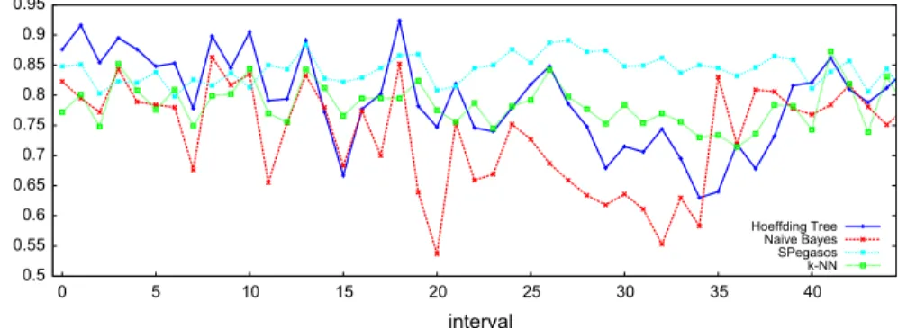
In this work we introduce a technique that natively combines heterogeneous models in the data stream setting. As data streams are constantly subject to change, the most accurate
classifier for a given interval of observations also changes frequently, as illustrated by Fig.1.
In their seminal paper,Littlestone and Warmuth(1994) describe a strategy to weight the
vote of ensemble members based on their performance on recent observations and prove certain error bounds. Although this work is of great theoretical value, it needs non-trivial adjustments to be applicable on practical data streams. Based on this approach, we propose a way to measure the performance of ensemble members on recent observations and combine their votes.
Our contributions are the following. We define Online Performance Estimation, a
frame-work that providesdynamicweighting of the votes of individual ensemble members across
the stream. Utilising this framework, we introduce a new ensemble technique that combines heterogeneous models. The members of the ensemble are selected based on their diversity
in terms of the correlation of their errors, leveraging theClassifier Output Difference(COD)
0.5 0.55 0.6 0.65 0.7 0.75 0.8 0.85 0.9 0.95
0 5 10 15 20 25 30 35 40
accuracy
interval
Hoeffding Tree Naive Bayes SPegasos k-NN
byPeterson and Martinez(2005). We conduct an extensive empirical study, covering 60 data streams and 25 classifiers, that shows that this technique is competitive with state of the art ensembles, while requiring significantly less resources. Our proposed methods are imple-mented in the data stream framework MOA and all our experimental results are made publicly available on OpenML.
The remainder of this paper is organised as follows. Section2surveys related work, and
Sect.3introduces the proposed methods. We demonstrate the performance by two
experi-ments. Section4describes the experimental setup, the selected data streams and the baselines.
Section5compares the performance of the proposed methods against state of the art methods,
and Sect.6surveys the effect of its parameters. Section7concludes.
2 Related work
It has been recognised that data stream mining differs significantly from conventional batch
data mining (e.g.,Domingos and Hulten 2003;Gama et al. 2009;Bifet et al. 2010a,b;Read
et al. 2012). In the conventional batch setting, a finite amount of stationary data is provided and the goal is to build a model that fits the data as well as possible. When working with data streams, we should expect an infinite amount of data, where observations come in one by one and are being processed in that order. Furthermore, the nature of the data can change
over time, known asconcept drift. Classifiers should be able to detect when a learned model
becomes obsolete and update it accordingly.
Common approachesSome batch classifiers can be trivially adapted to a data stream
set-ting. Examples arek Nearest Neighbour(Beringer and Hüllermeier 2007;Zhang et al.
2011), Stochastic Gradient Descent(Bottou 2004) andSPegasos
(Stochas-tic Primal Estimated sub-GrAdient SOlver for SVMs) (Shalev-Shwartz et al. 2011). Both
Stochastic Gradient Descent and SPegasos are gradient descent methods, capable of learning a variety of linear models, such as Support Vector Machines and Logistic Regression, depending on the chosen loss function.
Other classifiers have been created specifically to operate on data streams. Most
notably,Domingos and Hulten(2000) introduced theHoeffding Treeinduction
algo-rithm, which inspects every example only once, and stores per-leaf statistics to calculate theinformation gainon which the split criterion is determined. TheHoeffding boundstates that the true mean of a random variable of a given range will not differ from the estimated mean by more than a certain value. This provides statistical evidence that a certain split is
superior over others. AsHoeffding Treesseem to work very well in practice, many
vari-ants have been proposed, such asHoeffding Option Trees(Pfahringer et al. 2007),
Adaptive Hoeffding Trees(Bifet and Gavaldà 2009) andRandom Hoeffding Trees(Bifet et al. 2012).
Finally, a commonly used technique to adapt traditional batch classifiers to the data stream
setting is training them on a window ofwrecent examples: afterwnew examples have been
observed, a new model is built. This approach has the advantage that old examples are ignored, providing natural protection against concept drift. A disadvantage is that it doesn’t operate
directly on the most recently observed data, not beforewnew observations are made and the
model is retrained.Read et al.(2012) compare the performance of thesebatch-incremental
EnsemblesEnsemble techniques train multiple classifiers on a set of weighted training examples, and these weights can vary for different classifiers. In order to classify test
exam-ples, all individual models produce a prediction, also called avote, and the final prediction is
made according to a predefined voting schema, e.g., the class with the most votes is selected.
Based on Condorcet’s jury theorem (Hansen and Salamon 1990;Ladha 1993) there is
theo-retical evidence that the error rate of an ensemble in the limit goes to zero if two conditions are met. First, the individual models must do better than random guessing, and second, the individual models must be diverse, i.e., their errors should not be correlated.
Classifier Output Difference (COD) is a metric which measures the number of observations
on which a pair of classifiers yields a different prediction (Peterson and Martinez 2005). It
is defined as:
CODT(l1,l2)=
x∈T B(l1(x),l2(x))
|T| (1)
whereT is the set of all test instances,l1andl2are the classifiers to compare andl1(x)and
l2(x)is the label that the respective classifiersl1andl2give to test instancex; finally,Bis
a binary function that returns 1 iffl1(x)andl2(x)are equal and 0 otherwise.Peterson and
Martinez(2005) use this measure to ensure diversity among the ensemble members. A high value of COD indicates that two classifiers yield different predictions, hence they would be
well suited to combine in an ensemble.Lee and Giraud-Carrier(2011) use Classifier Output
Difference to build a hierarchical clustering among classifiers, resulting in classifiers that have similar predictions to be closely clustered, and vice versa.
In the data stream setting, ensembles can be eitherstaticordynamic. Static ensembles
contain a fixed set of ensemble members, whereas dynamic ensembles sometimes replace old models by new ones. Both approaches have advantages and disadvantages. Dynamic ensembles can actively replace obsolete models by new ones when concept drift occurs, whereas static ensembles need to rely on the individual members to recover from it. However, in order for dynamic ensembles to work properly, many parameters need to be set. For example, when to remove an old model, when to introduce a new model, which model should be introduced, and how long such new model should be trained before its vote will be considered. For these reasons, in this work we focus on static ensembles, in order to provide an off the shelf working method that does not require extensive parameter tuning. We will compare it with both static and dynamic ensemble methods.
Static ensemblesBagging (Breiman 1996) exploits the instability of classifiers by training
them on differentbootstrap replicates: resamplings (with replacement) of the training set.
Effectively, the training sets for various classifiers differ by the weights of their training
examples.Online Bagging(Oza 2005) operates on data streams by drawing the weight
of each example from aPoisson(1)distribution, which converges to the behaviour of the
classical Bagging algorithm if the number of examples is large. As the Hoeffding bound gives statistical evidence that a certain split criteria is optimal, this makes them more stable and hence less suitable for the use in a Bagging scheme. However, in practise this yields good
results. Boosting (Schapire 1990) is a technique that sequentially trains multiple classifiers,
in which more weight is given to examples that where misclassified by earlier classifiers.
Online Boosting(Oza 2005) applies this technique on data streams by assigning more weight to training examples that were misclassified by previously trained classifiers in the
ensemble. Stacking (Wolpert 1992;Gama and Brazdil 2000) combines heterogeneous models
in the classical batch setting. It trains multiple models on the training data. All base-learners
(2004) propose a hill-climbing method to select an appropriate set of base-learners from a large library of models.
Dynamic ensemblesWeighted Majorityis an ensemble technique specific to data
streams, where a meta-algorithm learns the weights of the ensemble members (Littlestone
and Warmuth 1994). The authors also provide tight error bounds compared for the
meta-algorithm compared to to the best ensemble member (under certain assumptions).Dynamic
Weighted Majorityis an extension of this work, specific to data streams with
chang-ing concepts (Kolter and Maloof 2007). It contains a set of classifiers, and measures the
performance of these based on recent observations. Whenever an ensemble member classi-fies a new observation wrong, its weight gets decreased by a predefined factor. Whenever the ensemble misclassifies an instance, a new ensemble member gets added to the pool of learners. Members with a weight below a given threshold get removed from the ensemble.
Accuracy Weighted Ensemble is an ensemble technique that splits the stream
into chunks of observations, and trains a classifier on each of these (Wang et al. 2003). Each
created classifier votes for a class-label, and the votes are weighted according to the expected error of the individual models. Poorly performing ensemble members are replaced by new
ones. As was remarked byRead et al. (2012), this makes them work particularly well in
combination with batch-incremental classifiers. Once a new model is built upon a batch of data, the old model will not be eliminated, but instead it is also used in the ensemble.
Meta-learningMeta-learning aims to learn which learning techniques work well on what
data. A common task, known as the Algorithm Selection Problem (Rice 1976), is to determine
which classifier performs best on a given dataset. We can predict this by training a meta-model on data describing the performance of different methods on different datasets, characterised bymeta-features(Brazdil et al. 1994). Meta-features are often categorised as either simple (number of examples, number of attributes), statistical (mean standard deviation of attributes, mean skewness of attributes), information theoretic (class entropy, mean mutual information),
or landmarkers, performance evaluations of simple classifiers (Pfahringer et al. 2000). In the
data stream setting, meta-learning techniques are often used to dynamically switch between classifiers at various points in the stream, effectively creating a heterogeneous ensemble (albeit at a certain cost in terms of resources).
Earlier approaches often train an ensemble of stream classifiers and a meta-model decides
for each data point which of the base-learners will make a prediction.Rossi et al.(2014)
dynamically choose between two regression techniques using meta-knowledge obtained
ear-lier in the stream.van Rijn et al.(2014) select the best classifier among multiple classifiers,
based on meta-knowledge from previously processed data streams. Online Performance
Esti-mation was first introduced byvan Rijn et al.(2015), which we will extend and improve in
this paper.Gama and Kosina(2014) uses meta-learning on time series with recurrent
con-cepts: when concept drift is detected, a meta-learning algorithm decides whether a model trained previously on the same stream could be reused, or whether the data is so different from
before that a new model must be trained. Finally,Nguyen et al.(2012) propose a method that
combines feature selection and heterogeneous ensembles; members that performed poorly can be replaced by a drift detector.
Concept driftOne property of data streams is that the underlying concept that is being
learned can change over time (e.g.,Wang et al. 2003). This is called concept drift. Some of
the aforementioned methods naturally deal with concept drift. For instance,k Nearest
Neighbourmaintains a number ofw recent examples, substituting each example after
w new examples have been observed.Change detectors, such as Drift Detection Method
combi-nation with any stream classifier. Both rely on the assumption that classifiers improve (or at least maintain) their accuracy when trained on more data. When the accuracy of a classifier drops with respect to a reference window, this could mean that the learned concept is outdated,
and a new classifier should be built. The main difference betweenDDMandADWINis the way
they select the reference window. Furthermore, classifiers can have built-in drift detectors.
For instance,Ultra Fast Forest of Trees(Gama et al. 2004b) areHoeffding
Treeswith a built-in change detector for every node. When an earlier made split turns out to be obsolete, a new split can be generated.
It has been recognised that some classifiers recover faster from sudden changes of concepts
than others.Shaker and Hüllermeier(2015) introducerecovery analysis, a framework to
measure the ability of classifiers to recover from concept drift. They distinguish
instance-based classifiers that operate directly on the data (e.g.,k-NN) and model-based classifiers, that
build and maintain a model (e.g., tree algorithms, fuzzy systems). Their experimental results suggest, quite naturally, that instance-based classifiers generally have a higher capability to recover from concept drift than model-based classifiers.
EvaluationAs data from streams is non-stationary, the well-known cross-validation pro-cedure for estimating model performance is not suitable. A commonly accepted estimation
procedure isthe prequential method(Gama et al. 2009), in which each example is first used
to test the current model, and afterwards (either directly after testing or after a delay) becomes available for training. An advantage of this method is that it is tested on all data, and therefore no specific holdout set is needed.
Experiment databasesExperiment databases facilitate the reproduction of earlier results for verification and reusability purposes, and make much larger studies (covering more clas-sifiers and parameter settings) feasible. Above all, experiment databases allow a variety of studies to be executed by a database look-up, rather than setting up new experiments. An
example of such an online experiment database is OpenML (Vanschoren et al. 2014). OpenML
is an Open Science platform for Machine Learning, containing many datasets, algorithms, and experimental results (the result of an algorithm on a dataset). For each experimental result it stores all predictions and class confidences, making it possible to calculate a wide range of measures, such as predictive accuracy and COD. We use OpenML to obtain infor-mation about the performance and interplay between various base-classifiers and to store our experimental results.
3 Methods
Traditional Machine Learning problems consist of a number ofexamplesthat are observed in
arbitrary order. In this work we consider classification problems. Each examplee=(x,l(x))
is a tuple of p predictive attributesx = (x1, . . . ,xp) and a target attributel(x). A data
set is an (unordered) set of such examples. The goal is to approximate a labelling function
l:x→l(x). In the data stream setting the examples are observed in a given order, therefore
each data streamSis a sequence of examplesS=(e1,e2,e3, . . . ,en, . . .), possibly infinite.
Consequently,eirefers to theit hexample in data streamS. The set of predictive attributes of
that example is denoted byPSi, likewisel(PSi)maps to the corresponding label. Furthermore,
the labelling function that needs to be learned can change over time due to concept drift. When applying an ensemble of classifiers, the most relevant variables are which base-classifiers (members) to use and how to weight their individual votes. This work mainly
c
w
l 0.7
l 0.7
l 0.8
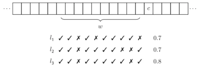
Fig. 2 Schematic view of Windowed Performance Estimation. For all classifiers,wflags are stored, each flag indicating whether it predicted a recent observation correctly
to weight member votes in an ensemble. In Sect.3.2we show how to use the Classifier Output
Difference to select ensemble members. Section3.3describes an ensemble that employs these
techniques.
3.1 Online performance estimation
In most common ensemble approaches all base-classifiers are given the same weight (as done in Bagging and Boosting) or their predictions are otherwise combined to optimise the overall performance of the ensemble (as done in Stacking). An important property of the data stream setting is often neglected: due to the possible occurrence of concept drift it is likely that in most cases recent examples are more relevant than older ones. Moreover, due to the fact that there is a temporal component in the data, we can actually measure how ensemble members have performed on recent examples, and adjust their weight in the voting accordingly. In order
to estimate the performance of a classifier on recent data,van Rijn et al.(2015) proposed:
Pwi n(l,c, w,L)=1− c−1
i=max(1,c−w)
L(l(PSi),l(PSi))
mi n(w,c−1) (2)
wherelis the learned labelling function of an ensemble member,cis the index of the last seen
training example andwis the number of training examples over which we want to estimate
the performance of ensemble members. Note that there is a certain start-up time (i.e., whenw
is larger than or equal toc) during which we can only calculate the performance estimation
over a number of instances smaller thanw. Also note that it can only be performed after
several labels have been observed (i.e.,c> 1). Finally,Lis a loss function that compares
the labels predicted by the ensemble member to the true labels. The most simple version is a zero/one loss function, which returns 0 when the predicted label is correct and 1 otherwise.
More complicated loss functions can also be incorporated. The outcome ofPwinis in the
range[0,1], with better performing classifiers obtaining a higher score. The performance
estimates for the ensemble members can be converted into a weight for their votes, at various points over the stream. For instance, the best performing members at that point could receive
the highest weights. Figure2illustrates this.
There are a few drawbacks to this approach. First, it requires the ensemble to store the
w×nadditional values, which is inconvenient in a data stream setting, where both time and
0 0.2 0.4 0.6 0.8 1
0 1000 2000 3000 4000 5000 6000 7000 8000 9000 10000
effect
observations
f(x) = 0.99 • f(x-1) f(x) = 0.999 • f(x-1) f(x) = 0.9999 • f(x-1)
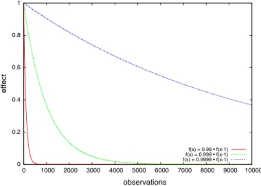
Fig. 3 The effect of a prediction after a number of observations, relative to when it was first observed (for various values ofα)
In order to address these issues, we propose an altered version of performance estimation,
based on fading factors, as described byGama et al.(2013). Fading factors give a high
importance to recent predictions, whereas the importance fades away when they become
older. This is illustrated by Fig.3.
The red (solid) line shows a relatively fast fading factor, where the effect of a given prediction is already faded away almost completely after 500 predictions, whereas the blue (dashed) line shows a relatively slow fading factor, where the effect of an observation is still
considerably high, even when 10,000 observations have passed in the meantime. Note that
even though all these functions start at 1, in practise we need to scale this down to 1−α, in
order to constrain the complete function within the range[0,1]. Putting this all together, we
propose:
P(l,c, α,L)=
1 iffc=0
P(l,c−1, α,L)·α+(1−L(l(PSc),l(PSc)))·(1−α)otherwise
(3)
where, similar to Eq.2,lis the learned labelling function of an ensemble member,c is
the index of the last seen training example andLis a loss function that compares the labels
predicted by the ensemble member to the true labels. Fading factorα(range[0,1]) determines
at what rate historic performance becomes irrelevant, and is to be tuned by the user. A value close to 0 will allow for rapid changes in estimated performance, whereas a value close
to 1 will keep them rather stable. The outcome of P is in the range [0,1], with better
performing classifiers obtaining a higher score. In Sect.6we will see that the fading factor
parameter is more robust and easier to tune than the window size parameter. When building an ensemble based upon Online Performance Estimation, we can now choose between a
Windowed approach (Eq.2) and Fading Factors (Eq.3).
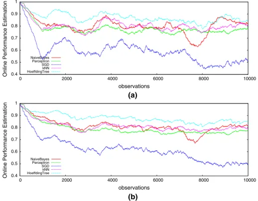
Figure4shows how the estimated performance for each base-classifier evolves at the start
0.4 0.5 0.6 0.7 0.8 0.9 1
0 2000 4000 6000 8000 10000
Online Performance Estimation
observations
NaiveBayes Perceptron SGD kNN HoeffdingTree
0.4 0.5 0.6 0.7 0.8 0.9 1
0 2000 4000 6000 8000 10000
Online Performance Estimation
observations
NaiveBayes Perceptron SGD kNN HoeffdingTree
(a)
(b)
Fig. 4 Online performance estimation, i.e. the estimated performance of each algorithm given previous examples, measured at the start of the electricity data stream.aWindowed, window size 1,000.bFading Factors,α=0.999
individual classifiers are measured. The Windowed approach contains many spikes, whereas the Fading Factor approach seems more stable.
3.2 Ensemble composition
In order for an ensemble to be successful, the individual classifiers should be both accurate and diverse. When employing a homogeneous ensemble, choosing an appropriate base-learner is an important decision. For heterogeneous ensembles this is even more true, as we have
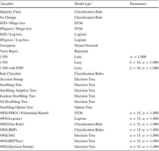
to choose a set of base-learners. We consider a set of classifiers from MOA 2016.04 (Bifet
et al. 2010a). Furthermore, we consider some fast batch-incremental classifiers from Weka
3.7.12 (Hall et al. 2009) wrapped in theAccuracy Weighted Ensemble(Wang et al.
2003). Table1lists all classifiers and their parameter settings.
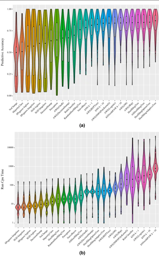
Figure5shows some basic results of the classifiers on 60 data streams. Figure5a shows
a violin plot of the predictive accuracy of all classifiers, with a box plot in the middle. Violin
plots show the probability density of the data at different values (Hintze and Nelson 1998).
0.00 0.25 0.50 0.75 1.00
NoChange MajorityClass
SPegasos logloss SPegasos hingeloss
SGD logloss SGD hingelossDecisionStump
PerceptronAWE(OneR)
AWE(DecisionStump) RuleClassifier
RandomHoeffdingTree NaiveBayeskNN k = 1
AWE(REPTree) kNN k = 10
AWE(SMO(PolyKernel)) AWE(Logistic)
kNNwithPAW k = 10 AWE(J48)AWE(JRip)
HoeffdingTree ASHoeffdingTree
HoeffdingOptionTree HoeffdingAdaptiveTree
Predictive Accuracy
1 10 100 1000 10000
SPegasos hingeloss SGD hingeloss
SPegasos logloss SGD logloss
DecisionStump NoChange
MajorityClassHoeffdingTree
RandomHoeffdingTree PerceptronNaiveBayes
ASHoeffdingTree AWE(OneR)
AWE(DecisionStump)HoeffdingOptionTree HoeffdingAdaptiveTree
AWE(REPTree) AWE(J48)AWE(JRip)
AWE(SMO(PolyKernel)) RuleClassifier
kNN k = 1 AWE(Logistic)
kNN k = 10
kNNwithPAW k = 10
Run Cpu Time
(a)
(b)
Table 1 Classifiers considered in this research
Classifier Model type Parameters
Majority Class Classification Rule
No Change Classification Rule
SGD / Hinge loss SVM
SPegasos / Hinge loss SVM
SGD / Log loss Logistic
SPegasos / Log loss Logistic
Perceptron Neural Network
Naive Bayes Bayesian
1-NN Lazy w=1,000
k-NN Lazy k=10,w=1,000
k-NN with PAW Lazy k=10,w=1,000
Rule Classifier Classification Rules
Decision Stump Decision Tree
Hoeffding Tree Decision Tree
Hoeffding Adaptive Tree Decision Tree
Random Hoeffding Tree Decision Tree
AS Hoeffding Tree Decision Tree
Hoeffding Option Tree Option Tree
AWE(SMO) / Polynomial Kernel SVM n=15, w=1,000
AWE(Logistic) Logistic n=15, w=1,000
AWE(One Rule) Classification Rule n=15, w=1,000
AWE(JRIP) Classification Rules n=15, w=1,000
AWE(J48) Decision Tree n=15, w=1,000
AWE(REPTree) Decision Tree n=15, w=1,000
AWE(Decision Stump) Decision Tree n=15, w=1,000
All parameters are set to default values, unless specified otherwise
Figure 5b shows violin plots of the run time (in seconds) that the classifiers needed
to complete the tasks. From the top-half performing classifiers in terms of accuracy, the
Hoeffding Treesis the best ranked algorithm in terms of run time. Lazy algorithms
(k-NN and its variations) turn out to be rather slow, despite the reasonable value of window
size parameter (controlling the number of instances that are remembered). It also confirms
some observation made byRead et al.(2012), that the batch-incremental classifiers
gener-ally take more resources than instance-incremental classifiers; all classifiers wrapped in the
Accuracy Weighted Ensembleare on the right half of the figure.
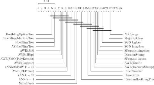
Figure6shows the result of a statistical test on the base-classifiers. Classifiers are sorted
by their average rank (lower is better). Classifiers that are connected by a horizontal line are statistically equivalent. The results confirm some of the observations made based on the violin
plots, e.g., the baseline models (Majority ClassandNo Change) perform worst; also
other simple models such as theDecision StumpsandOneRule(which is essentially
a Decision Stump) are inferior to the tree-based models. Oddly enough, the instance
incre-mentalRule Classifierdoes not compete at all with the Batch-incremental counterpart
Fig. 6 Results of Nemenyi test (α=0.05) on the predictive accuracy of the base-classifiers in this study
When creating a heterogeneous ensemble, a diverse set of classifiers should be
selected (Hansen and Salamon 1990). Classifier Output Difference is a metric that
mea-sures the difference in predictions between a pair of classifiers. We can use this to create a
hierarchical agglomerative clustering of data stream classifiers in an identical way toLee
and Giraud-Carrier(2011). For each pair of classifiers involved in this study, we measure the number of observations for which the classifiers have different outputs, aggregated over all data streams involved. Hierarchical agglomerative clustering (HAC) converts this informa-tion into a hierarchical clustering. It starts by assigning each observainforma-tion to its own cluster, and
greedily joins the two clusters with the smallest distance (Rokach and Maimon 2005). The
complete linkage strategy is used to measure the distance between two clusters. Formally, the
distance between two clustersAandBis defined asmax{COD(a,b):a∈A,b∈B}.
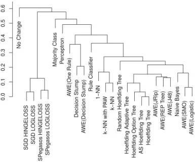
Fig-ure7shows the resulting dendrogram. There were 9 data streams on which several classifiers
did not terminate. We left these out of the dendrogram.
We can use a dendrogram like the one in Fig.7to get a collection of diverse and well
per-forming ensemble members. A COD-threshold is to be determined, selecting representative classifiers from all clusters with a distance lower than this threshold. A higher COD-threshold would result in a smaller set of classifiers, and vice versa. For example, if we set the
COD-threshold to 0.2, we end up with an ensemble consisting of classifiers from 11 clusters. The
ensemble will consist of one representative classifier from each cluster, which can be
cho-sen based on accuracy, run time, a combination of the two (e.g.,Brazdil et al. 2003) or any
arbitrary other criteria. Which exact criteria to use is outside the scope of this research, how-ever in this study we used a combination of accuracy and run time. Clearly, when using this technique in experiments, the dendrogram should be constructed in a leave-one-out setting: it can be created based on all data streams except for the one that is being tested.
Figure7can also be used to make some interesting observations. First, it confirms some
well-established assumptions. The clustering seems to respect the taxonomy of classifiers pro-vided by MOA. Many of the tree-based and rule-based classifiers are grouped together. There
is a cluster of instance-incremental tree classifiers (Hoeffding Tree,AS Hoeffding
Fig. 7 Hierarchical clustering of stream classifiers, averaged over 51 data streams from OpenML
batch-incremental tree-based and rule-based classifiers (REP Tree,J48andJRip) and
a cluster of simple tree-based and rule-based classifiers (Decision StumpsandOne
Rule). Also the Logistic and SVM models seem to produce similar predictions, having
a sub-cluster of batch-incremental classifiers (SMOandLogistic) and a sub-cluster of
instance incremental classifiers (Stochastic Gradient DescentandSPegasos
with both loss functions).
The dendrogram also provides some surprising results. For example, the
instance-incrementalRule Classifierseems to be fairly distant from the tree-based classifiers.
As decision rules and decision trees work with similar decision boundaries and can easily be
translated to each other, a higher similarity would be expected (Apté and Weiss 1997). Also
the internal distances in the simple tree-based and rule-based classifiers seem rather high.
A possible explanation for this could be the mediocre performance of the Rule
Classifier(see Fig. 5). Even though COD clusters are based on instance-level pre-dictions rather than accuracy, well performing classifiers have a higher prior probability of being clustered together. As there are only few observations they predict incorrectly, naturally there are also few observations their predictions can disagree on.
3.3 BLAST
BLAST(short forbestlast) is an ensemble embodying the performance estimation frame-work. Ideally, it consists of a group of diverse base-classifiers. These are all trained using the full set of available training observations. For every test example, it selects one of its
mem-bers to make the prediction. This member is referred to as theactive classifier. The active
classifier is selected based on Online Performance Estimation: the classifier that performed
best over the set ofw previous training examples is selected as the active classifier (i.e., it
gets 100% of the weight), hence the name. Formally,
ACc=arg max
mj∈M
Algorithm 1BLAST (Learning)
Require:Set of ensemble membersM, Loss functionLand Fading Factorα 1: Initialise ensemble membersmj, withj∈ {1,2,3, . . . ,|M|}
2: Setpj=1 for allj
3:for alltraining examplese=(x,l(x))do
4: for allmj∈Mdo
5: lj(x)←predicted label ofmjon attributesxof current examplee
6: pj←pj·α+(1−L(lj(x),l(x)))·(1−α)
7: Updatemjwith current examplee
8: end for
9:end for
whereMis the set of models generated by the ensemble members,cis the index of the
cur-rent example,α is a parameter to be set by the user (fading factor) and L is a zero/one
loss function, giving a penalty of 1 to all misclassified examples. Note that the
perfor-mance estimation function Pcan be replaced by any measure. For example, if we would
replace it with Eq.2, we would get the exact same predictions as reported byvan Rijn
et al.(2015). When multiple classifiers obtain the same estimated performance, any arbitrary classifier can be selected as active classifier. The details of this method are summarised in
Algorithm1.
Line 2 initialises a variable that keeps track of the estimated performance for each base-classifier. Everything that happens from lines 5–7 can be seen as an internal prequential evaluation method. At line 5 each training example is first used to test all individual
ensem-ble members on. The predicted label is compared against the true labell(x) on line 7.
If it predicts the correct label then the estimated performance for this base-classifier will increase; if it predicts the wrong label, the estimated performance for this base-classifier
will decrease (line 6). After this, base-classifier mj can be trained with the example
(line 7). When, at any time, a test example needs to be classified, the ensemble looks up
the highest value of pj and lets the corresponding ensemble member make the
predic-tion.
The concept of an active classifier can also be extended to multiple active classifiers.
Rather than selecting the best classifier on recent predictions, we can select the bestk
classi-fiers, whose votes for the specified class-label are all weighted according to some weighting schedule. First, we can weight them all equally. Indeed, when using this voting schedule and
settingk = |M|, we would get the same behaviour as theMajority Vote Ensemble,
as described byvan Rijn et al.(2015), which performed only averagely. Alternatively, we
can use Online Performance Estimation to weight the votes. This way, the best performing classifier obtains the highest weight, the second best performing classifier a bit less, and so
on. Formally, for eachy∈Y(withYbeing the set of all class labels):
votesy=
mj∈M
P(mj,i, α,L)×B(lj(PSi),y) (5)
whereM is the set of all models,lj is the labelling function produced by modelmj and
B is a binary function, returning 1 ifflj voted for class label y and 0 otherwise. Other
functions regulating the voting process can also be incorporated, but are beyond the scope of
this research. The labelythat obtained the highest valuevotesyis then predicted.BLASTis
4 Experimental setup
In order to establish the utility ofBLASTand Online Performance Estimation, we conduct
experiments using a large set of data streams. The data streams and results of all experiments are made publicly available in OpenML for the purposes of verifiability, reproducibility and
generalizability.1
Data streamsThe data streams are a combination of real world data streams (e.g., elec-tricity, covertype, IMDB) and synthetically generated data (e.g., LED, Rotating Hyperplane,
Bayesian Network Generator) commonly used in data stream research (e.g.,Beringer and
Hüllermeier 2007;Bifet et al. 2010a;van Rijn et al. 2014). Many contain a natural drift
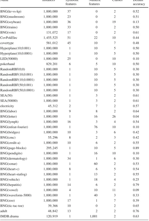
of concept. Table2shows a list of all data streams, the number of observations, features,
classes and their default accuracy. We estimate the performance of the methods using the prequential method: each observation is used as a test example first and as a training example
afterwards (Gama et al. 2009). As most data streams are fairly balanced, we will measure
predictive accuracy in the experiments.
BaselinesWe compare the results of the defined methods with theBest Single Classifier.
Each heterogeneous ensemble consists ofn base-classifiers. The one that performs best
on average over all data streams is considered theBest Single Classifier. This
will allow to measure the potential accuracy gains of adding more classifiers (at the cost of using more computational resources). Which classifier should be considered the best
single classifier is debatable. Based on the median scores depicted in Fig.5a,Hoeffding
Adaptive Treeis the best performing classifier. Based on the statistical test depicted in
Fig.6, theHoeffding Option Treeis the best performing classifier. We selected the
Hoeffding Option Treeas the single best classifier.
Furthermore, we compare against the Majority Vote Ensemble, which is a
heteroge-neous ensemble that predicts the label that is predicted by most ensemble members. This allows to measure the potential accuracy gain of using Online Performance Estimation over just naively combining the votes of individual classifiers. Finally, we also compare
the techniques to state of the art homogeneous ensembles, such asOnline Bagging,
Leveraging Bagging, andAccuracy Weighted Ensemble. These are
embod-ied with aHoeffding Treeas base-classifier, because this is a good trade-off between
predictive performance and run time. Amongst all classifiers that are considered statistically
equivalent with the best classifier (Fig.6on page 14), it has the lowest median run time
(Fig.5b on page 13). This beneficial trade-off was also noted byDomingos and Hulten
(2003), andRead et al.(2012), and allows for the use of a high number of base-classifiers.
In order to understand the performance of these ensembles a bit better, we provide some results.
Figure8shows violin plots of the performance ofAccuracy Weighted Ensemble
(left bars, red),Leveraging Bagging (middle bars, green) andOnline Bagging
(right bars, blue), with an increasing number of ensemble members.Accuracy Weighted
Ensemble (AWE) uses J48 trees as ensemble members, both Bagging schemes use
Hoeffding Trees. Naturally, as the number of members increases, both accuracy and
run time increase, howeverLeveraging Baggingperforms eminently better than the
others.Leveraging Baggingusing 16 ensemble members already outperforms both
AWEandOnline Bagging using 128 ensemble members, based on median accuracy. This performance also comes at a cost, as it uses considerably more run time than both other
techniques, even when containing the same number of members.Accuracy Weighted
Table 2 Data streams used in the experiment
Name Instances Symbolic
features
Numeric features
Classes Default accuracy
BNG(kr-vs-kp) 1,000,000 37 0 2 0.52
BNG(mushroom) 1,000,000 23 0 2 0.51
BNG(soybean) 1,000,000 36 0 19 0.13
BNG(trains) 1,000,000 33 0 2 0.50
BNG(vote) 131,072 17 0 2 0.61
CovPokElec 1,455,525 51 22 10 0.44
covertype 581,012 45 10 7 0.48
Hyperplane(10;0.001) 1,000,000 1 10 5 0.50
Hyperplane(10;0.0001) 1,000,000 1 10 5 0.50
LED(50000) 1,000,000 25 0 10 0.10
pokerhand 829,201 6 5 10 0.50
RandomRBF(0;0) 1,000,000 1 10 5 0.30
RandomRBF(10;0.001) 1,000,000 1 10 5 0.30
RandomRBF(10;0.0001) 1,000,000 1 10 5 0.30
RandomRBF(50;0.001) 1,000,000 1 10 5 0.30
RandomRBF(50;0.0001) 1,000,000 1 10 5 0.30
SEA(50) 1,000,000 1 3 2 0.61
SEA(50000) 1,000,000 1 3 2 0.61
electricity 45,312 2 7 2 0.57
BNG(labor) 1,000,000 9 8 2 0.64
BNG(letter) 1,000,000 1 16 26 0.04
BNG(lymph) 1,000,000 16 3 4 0.54
BNG(mfeat-fourier) 1,000,000 1 76 10 0.10
BNG(bridges) 1,000,000 10 3 6 0.42
BNG(cmc) 55,296 8 2 3 0.42
BNG(credit-a) 1,000,000 10 6 2 0.55
BNG(page-blocks) 295,245 1 10 5 0.89
BNG(pendigits) 1,000,000 1 16 10 0.10
BNG(dermatology) 1,000,000 34 1 6 0.30
BNG(sonar) 1,000,000 1 60 2 0.53
BNG(heart-c) 1,000,000 8 6 5 0.54
BNG(heart-statlog) 1,000,000 1 13 2 0.55
BNG(vehicle) 1,000,000 1 18 4 0.25
BNG(hepatitis) 1,000,000 14 6 2 0.79
BNG(vowel) 1,000,000 4 10 11 0.09
BNG(waveform-5000) 1,000,000 1 40 3 0.33
BNG(zoo) 1,000,000 17 1 7 0.39
BNG(tic-tac-toe) 39,366 10 0 2 0.65
adult 48,842 13 2 2 0.76
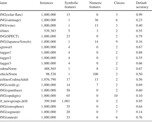
Table 2 continued
Name Instances Symbolic
features
Numeric features
Classes Default accuracy
BNG(solar-flare) 1,000,000 13 0 3 0.99
BNG(satimage) 1,000,000 1 36 6 0.23
BNG(wine) 1,000,000 1 13 3 0.40
airlines 539,383 5 3 2 0.55
BNG(SPECT) 1,000,000 23 0 2 0.79
BNG(JapaneseVowels) 1,000,000 1 14 9 0.16
Agrawal1 1,000,000 4 6 2 0.67
Stagger1 1,000,000 4 0 2 0.88
Stagger2 1,000,000 4 0 2 0.55
Stagger3 1,000,000 4 0 2 0.66
codrnaNorm 488,565 1 8 2 0.67
vehicleNorm 98,528 1 100 2 0.50
AirlinesCodrnaAdult 1,076,790 17 13 2 0.56
BNG(credit-g) 1,000,000 14 7 2 0.69
BNG(spambase) 1,000,000 58 0 2 0.60
BNG(optdigits) 1,000,000 65 0 10 0.10
20_newsgroups.drift 399,940 1,001 0 2 0.95
BNG(ionosphere) 1,000,000 35 0 2 0.64
BNG(segment) 1,000,000 20 0 7 0.14
BNG(anneal) 1,000,000 33 6 6 0.76
All are obtained from OpenML
Ensembleperforms pretty constant, regardless of the amount of ensemble members. As the
ensemble size grows, both accuracy and run time slightly increase. We will compareBLAST
against the heterogeneous ensembles containing 128 ensemble members.
Ensemble membersWe evaluate an instantiation ofBLAST, using a set of differing
classi-fiers. These are selected using the dendrogram from Fig.7, setting theCODthreshold to 0.2.
Using this threshold, it recommends a set of 12 classifiers. After omitting simple models such asNo Change,Majority ClassandDecision Stumps, we end up with the set of
classifiers described in Table3. One nice property is that all base-classifiers consist of
dif-ferent model types, making the resulting ensemble very heterogeneous. As for the baselines,
Majority Vote Ensembleuses the same classifiers.
5 Results
We ran all ensemble techniques on all data streams.BLASTwas run both with fading factors
(α=0.999) and Windowed (w=1,000). For each prediction, one classifier was selected as
the active classifier (i.e.,k =1). We explore the effect of other values for both parameters in
Section6.
Figure9a shows violin plots and box plots of the results in terms of accuracy. An important
(a)
(b)
Fig. 8 Effect of the number of ensemble members on performance of Online Bagging and Leveraging Bagging.
aAccuracy.bRun time (in seconds)
Table 3 Classifiers used in the experiment
Classifier Model type Parameters
Naive Bayes Bayesian
Stochastic Gradient Descent SVM Loss function: Hinge
kNearest Neighbour Lazy k=10,w=1,000
Hoeffding Option Tree Option Tree
Perceptron Neural Network
Random Hoeffding Tree Decision Tree
Rule Classifier Decision Rules
0.25 0.50 0.75 1.00
Majority Vote Ensemble AWE(J48)
Best Single Classifier Online Bagging
BLAST (Window) BLAST (FF)
Leveraging Bagging
Predictive Accuracy
1 10 100 1000 10000
Best Single Classifier AWE(J48)
Majority Vote Ensemble BLAST (Window)
BLAST (FF) Online Bagging
Leveraging Bagging
Run Cpu Time
(a)
(b)
Fig. 9 Performance of the proposed techniques averaged over 60 data streams.aAccuracy.bRun time (in seconds)
The highest median score is obtained byLeveraging Bagging, which performs very
well in various empirical studies (Bifet et al. 2010b; Read et al. 2012; van Rijn 2016),
closely followed by both versions ofBLAST. Both versions ofBLASThave less outliers at
the bottom thanLeveraging Bagging. AsLeveraging Baggingsolely relies on
Hoeffding Treesas base-classifier, it will perform averagely on datasets that are not
easily modelled by trees. Contrarily,BLASTeasily selects an appropriate set of classifiers
for each dataset, hence the fewer number of outliers.
As expected, both the Best Single Classifier and the Majority Vote
results from some ensemble members outweigh the diversity. A peculiar observation is that theAccuracy Weighted Ensemble, which utilises historic performance data in a
dif-ferent way, does not manage to outperform theBest Single Classifier. Possibly,
the window of 1,000 instances on which the individual classifiers are trained is too small to
make the individual models competitive.
Figure9b shows plots of the results in terms of run time on a log scale. The results are
as expected. TheBest Single Classifier requires fewest resources, followed by
AWE(J48). AlthoughAWE(J48)consists of 128 ensemble members, it essentially feeds
each training instance to just one ensemble member. TheMajority Vote Ensemble
and both versions ofBLASTalso require a similar amount of resources, as these already use
the classifiers mentioned in Table3. Finally, both Bagging ensembles require most resources,
which was also observed byBifet et al.(2010b) andRead et al.(2012). The fact thatBLAST
performs competitively with the Bagging ensemble, while it requires far fewer resources, suggests that Online Performance Estimation is a useful technique when applied to hetero-geneous data stream ensembles.
Figure10shows the accuracy of the three heterogeneous ensemble techniques per data
stream. In order to not overload the figure, we only showBLASTwith fading factors (FF),
Leveraging Baggingand theBest Single Classifier.
BothBLAST (FF)andLeveraging Baggingconsistently outperform theBest Single Classifier. Especially on data streams where the performance of theBest Single Classifieris mediocre (Fig.10b), accuracy gains are eminent. The difference
betweenLeveraging BaggingandBLASTis harder to assess. AlthoughLeveraging
Baggingseems to be slightly better in many cases, there are some clear cases where there
is a big difference in favour ofBLAST.
To assess statistical significance, we use the Friedman test with post-hoc Nemenyi test to establish the statistical relevance of our results. These tests are considered the state of
the art when it comes to comparing multiple classifiers (Demšar 2006). The Friedman test
checks whether there is a statistical difference between the classifiers; when this is the case the Nemenyi post-hoc test can be used to determine which classifiers are significantly better than others.
The results of the Nemenyi test (α = 0.05) are shown in Fig.11. It plots the average
rank of all methods and the critical difference. Classifiers that are statistically equivalent are connected by a black line. For all other cases, there was a significant difference in performance, in favour of the classifier with the better average rank. We performed the test based on accuracy and run time.
Figure11a shows that there is no statistically significant difference in terms of accuracy
betweenBLAST(FF) and the homogeneous ensembles (i.e.,Leveraging Baggingand
Online Baggingusing 128Hoeffding Trees).BLAST (Window)does perform
significantly worse thanLeveraging Bagging.2Similar to Fig.9a, theBest Single
Classifier,AWE(J48)andMajority Vote Ensembleare at the bottom of the ranking. These perform significantly less than the other techniques.
Figure11b shows the results of the Nemenyi test on run time. The results are similar to
Fig.9b. The best single classifier (Hoeffding Option Tree) requires fewest resources.
There is no significant difference in resources betweenBLAST (FF),BLAST (Window),
Majority Vote EnsembleandOnline Bagging. This makes sense, as these the
2van Rijn et al.(2015) reported statistical equivalence between the Windowed version andLeveraging Bagging, however their experimental setup was different:BLASTcontained a set of 11 base-classifiers and
0.84 0.86 0.88 0.9 0.92 0.94 0.96 0.98 1
Stagger3Stagger1Stagger2BNG(mushroom)BNG(dermatology)BNG(vote)20_newsgroups.driftcodrnaNormBNG(kr-vs-kp)Agrawal1BNG(ionosphere)BNG(anneal)BNG(labor)BNG(trains)BNG(wine)BNG(zoo)BNG(SPECT)BNG(hepatitis)BNG(optdigits)BNG(lymph)BNG(page-blocks)BNG(soybean)Hyperplane(10;0.0001)BNG(heart-statlog)BNG(heart-c)BNG(credit-a)BNG(waveform-5000)BNG(segment)covertypeSEA(50000)
Best Single Classifier Leveraging Bagging BLAST (FF)
(a)
0.3 0.4 0.5 0.6 0.7 0.8 0.9 1
SEA(50)BNG(mfeat-fourier)adultRandomRBF(0;0)electricityvehicleNormBNG(satimage)BNG(pendigits)CovPokElecBNG(sonar)RandomRBF(10;0.0001)Hyperplane(10;0.001)BNG(JapaneseVowels)AirlinesCodrnaAdultBNG(credit-g)RandomRBF(10;0.001)pokerhandBNG(tic-tac-toe)BNG(solar-flare)BNG(vowel)LED(50000)BNG(bridges)BNG(spambase)BNG(vehicle)airlinesIMDB.dramaRandomRBF(50;0.0001)BNG(cmc)BNG(letter)RandomRBF(50;0.001)
Best Single Classifier Leveraging Bagging BLAST (FF)
(b)
Fig. 10 Accuracy per data stream, sorted by accuracy of the best single classifier
first three operate on the same set of base-classifiers. Altogether,BLAST (FF)performs
equivalent to both Bagging schemes in terms of accuracy, while using significantly fewer resources.
6 Parameter effect
(a)
(b)
Fig. 11 Results of Nemenyi test,α=0.05. Classifiers are sorted by their average rank (lower is better). Classifiers that are connected by a horizontal line are statistically equivalent.aAccuracy.bRun time
0.6 0.8 1.0
a = 0.9
w = 10 a = 0.99w = 100 a = 0.999
w = 1000 a = 0.9999w = 10000
Predictiv
e A
ccuracy
BLAST (FF) BLAST (Window)
Fig. 12 Effect of the decay rate and window parameter
6.1 Window size and decay rate
First, for both versions ofBLAST, there is a parameter that controls the rate of dismissal of
old observations. ForBLAST (FF)this is theαparameter (the fading factor); forBLAST
(Windowed)this is thewparameter (the window size). Theαparameter is always in the
range[0,1], and has no effect on the use of resources. The window parameter can be in the
range[0,n], wherenis the size of the data stream. Setting this value higher results in bigger
0.5 0.6 0.7 0.8 0.9 1.0
g = 1 g = 10
g = 100 g = 1000
Predictiv
e A
ccuracy
BLAST (FF) BLAST (Window)
Fig. 13 Effect of the grace parameter on accuracy. Thex-axis denotes the grace, they-axes the performance.
BLAST (Window)was run withw=1,000;BLAST (FF)was run withα=0.999
Figure12shows violin plots and box plots of the effect of varying these parameters. The
effect of theα(a) value onBLAST (FF)is displayed in the left (red) violin plots; the effect
of the window (w) value onBLAST (Window)is displayed in the right (blue) violin plots.
The trend over 60 data streams seems to be that setting this parameter too low results in
sub-optimal accuracy. This is especially clear withBLAST (FF)withα=0.9 andBLAST
(Window)withw=10: there are more outliers at the bottom and the third quartile of the box plot is slightly larger. Arguably, this value performs well in highly volatile streams when concepts change rapidly, but in general we do not want to dismiss old information too quickly. In the other cases, the higher values seem to be slightly preferred, but it is hard to draw general
conclusions from this. Altogether,BLAST (FF)seems to be slightly more robust, as the
investigated values of theαparameter do not perceptibly influence performance.
6.2 Grace parameter
Prior work byRossi et al.(2014) andvan Rijn et al.(2015) introduced a grace parameter that
controls the number of observations for which the active classifier was not changed. This potentially saves resources, especially when the algorithm selection process involves time consuming operations such as the calculation of meta-features. On the other hand, it can be seen that in a data stream setting where concept drift occurs, in terms of performance it is always optimal to act on changed behaviour as fast as possible. Although we have omitted this
parameter from the formal definition ofBLASTin Sect.3, similar behaviour can be obtained
by updating the active classifier only at certain intervals. Formally, a grace period can be
enforced by only executing Eq.4whenc mod g=0, where (following earlier definitions)
cis the index of the current observation, andgis a grace period defined by the user.
Figure13shows the effect of the (hypothetical) grace parameter on performance, averaged
over 60 data streams. We observe two things from this plot. First, the difference in performance for various values of this parameter is quite small. Second, although this difference is very small, it seems that lower values are preferred.
The fact that the differences are small is supported by intuition. Although the performance ranking of the classifiers varies over the stream, it only happens occasionally that a new best
it is still the case that the old active classifier will probably not be entirely outdated. It will still predict with reasonable accuracy, until it is replaced. The fact that smaller values are preferable also makes sense. In data streams that contain concept drift, it is desirable to immediately act on the observed changes. Therefore, having a grace parameter can only
affect performance in a negative way. Moreover, the algorithm selection phase of BLAST
simply depends on finding the maximum element in an array. For these reasons, the grace period would not have any measurable influence on the required resources, and its default value can be fixed to 1.
6.3 Number of active classifiers
Rather than selecting one active classifier, multiple active classifiers can be selected that all vote for a class label. The votes of these classifiers can either contribute equally to the final
vote, or be weighted according to their estimated performance. We usedBLAST (FF)to
explore the effect of this parameter. We varied the number of active classifierskfrom one to
five, and measured the performance according to both voting schemas. Figure14shows the
results.
Figure14a shows how the various strategies perform when evaluated using predictive
accuracy. We can make several observations to verify the correctness of the results. First, the
results of both strategies are equal whenk=1, as the algorithm selects only one classifier,
weights are obsolete. Second, the result of the Majority weighting schema fork=7 is equal
to the score of theMajority Weight Ensemble(from Fig.9a), which is also correct,
as these are the same by definition. Finally, when using the weighted strategy, settingk=2
yields exactly the same scores for accuracy as settingk = 1. This also makes sense, as
it is guaranteed that the second best base-classifier always has a lower weight as the best base-classifier, and thus it is incapable of changing any prediction.
In all, it seems that increasing the number of active classifiers is not beneficial for accuracy. Note that this is different from adding more classifiers in general, which clearly would not decrease performance results. This behaviour is different from the classical approach, where adding more classifiers (which inherently are all active) yield better results up to a
certain point (Caruana et al. 2004). However, in the data stream setting we deal with a time
component, and we can actually measure which classifiers performed well on recent intervals. By increasing the number of active classifiers, we would add classifiers to the vote of which we have empirical evidence that they performed worse on recent observations.
Similarly, Fig.14b shows the Root Mean Squared Error (RMSE). RSME is typically used
as an evaluation measure for regression, but can be used in classification problems to assess the quality of class confidences. For every prediction, the error is considered to be the difference between the class confidence for the correct label and 1. This means that if the classifier had a confidence close to 1 for the particular class label, a low error is recorded, and vice versa. The box plots indicate that adding more active classifiers can lead to a lower median error. This also makes sense, as the Root Mean Squared Error tends to punish classification errors
harder when these are made with a high confidence. We observe this effect untilk =3, after
which adding more active classifiers starts to lead to a higher RMSE. It is unclear why this effect holds until this particular value.
0.4 0.6 0.8 1.0
k = 1 k = 2 k = 3 k = 4 k = 5 k = 6 k = 7
Predictive Accuracy
0.0 0.2 0.4 0.6
k = 1 k = 2 k = 3 k = 4 k = 5 k = 6 k = 7
Root Mean Squared Error
Majority Weighted
Majority Weighted
(a)
(b)
Fig. 14 Performance for various values ofk, weighted votes versus unweighted votes.aAccuracy.bRoot Mean Squared Error
classifiers, this is considered future work. Clearly, when using multiple active classifiers, weighting their votes using online performance estimation seems beneficial.
7 Conclusions
factors, which considers all predictions from the whole stream, but gives a higher weight to recent predictions.
BLASTis an heterogeneous ensemble technique based on Online Performance Estimation that selects the single best classifier on recent predictions to classify new observations. We
have integrated both performance estimation functions intoBLAST. Empirical evaluation
shows thatBLASTwith fading factors performs better thanBLASTusing the windowed
approach. This is most likely because Fading Factors are better able to capture typical data stream properties, such as changes of concepts. When this occurs, there will also be changes in the performances of ensemble members, and the fading factors adapt to this relatively fast.
We compared BLAST against state of the art ensembles over 60 data streams from
OpenML. To the best of our knowledge, this is the largest data stream study to date. We observe that there is no statistical significant difference between the accuracy of the
ensem-bles, althoughBLASTuses significantly fewer resources. Furthermore, we evaluated the
effect of the method’s parameters on the performance. The most important parameter proves
to be the one controlling the performance estimation function:αfor the fading factor,
con-trolling the decay rate, andwfor the windowed approach, determining the window size. Our
results show that the optimal value for these parameters is dependent on the given dataset, although setting this too low turns out to have a worse effect on accuracy than setting it too high.
To select the classifiers included in the heterogeneous ensemble, we created a hierarchical clustering of 25 commonly used data stream classifiers, based on Classifier Output Difference. We used this clustering to gain methodological justification for which classifiers to use, although the clustering is mainly a guideline. A human expert can still determine to deviate from the resulting set of algorithms, in order to save resources. The resulting dendrogram has also scientific value in itself. It confirms some well-established assumptions regarding the typically used classifier taxonomy in data streams, that have never been tested before. Many of the classifiers that were suspected to be similar were also clustered together, for example the various decision trees, support vector machines and gradient descent models all formed their own clusters. Moreover, some interesting observations were made that can be investigated in future work. For instance, the Rule Classifier used turns out to perform averagely, and was rather far removed from the decision trees, whereas we would expect it to perform better and be clustered closer to the decision trees.
Utilizing the Online Performance Estimation framework opens up a whole new line of data stream research. Rather than creating more data stream classifiers, combining them in a suitable way can elegantly lead to highly improved results that effortlessly adapt to changes in the data stream. More than in the classical batch setting, memory and time are of crucial importance. Experiments suggest that the selected set of base classifiers has a substantial influence on the performance of the ensemble. Research should be conducted to explore what model types best complement each other, and which work well together given a constraint on resources. We believe that by exploring these possibilities we can further push the state of the art in data stream ensembles.
Acknowledgements This work is supported by Grant 612.001.206 from the Netherlands Organisation for Scientific Research (NWO) and by the Emmy Noether Grant HU 1900/2-1 from the German Research Foun-dation (DFG).
References
Apté, C., & Weiss, S. (1997). Data mining with decision trees and decision rules.Future Generation Computer Systems,13(2), 197–210.
Beringer, J., & Hüllermeier, E. (2007). Efficient instance-based learning on data streams.Intelligent Data Analysis,11(6), 627–650.
Bifet, A., Frank, E., Holmes, G., & Pfahringer, B. (2012). Ensembles of restricted hoeffding trees.ACM Transactions on Intelligent Systems and Technology (TIST),3(2), 30.
Bifet, A., & Gavalda, R. (2007). Learning from time-changing data with adaptive windowing.SDM, SIAM,7, 139–148.
Bifet, A., & Gavaldà, R. (2009). Adaptive learning from evolving data streams. InAdvances in intelligent data analysis VIII(pp. 249–260). Springer.
Bifet, A., Holmes, G., Kirkby, R., & Pfahringer, B. (2010a). MOA: Massive online analysis.Journal of Machine Learning Research,11, 1601–1604.
Bifet, A., Holmes, G., & Pfahringer, B. (2010b). Leveraging bagging for evolving data streams. InMachine learning and knowledge discovery in databases, Lecture Notes in Computer Science(Vol. 6321, pp. 135–150). Springer.
Bottou, L. (2004). Stochastic learning. InAdvanced lectures on machine learning(pp. 146–168). Springer. Brazdil, P., Gama, J., & Henery, B. (1994). Characterizing the applicability of classification algorithms using
meta-level learning. InMachine learning: ECML-94(pp. 83–102). Springer.
Brazdil, P., Soares, C., & Da Costa, J. P. (2003). Ranking learning algorithms: Using IBL and meta-learning on accuracy and time results.Machine Learning,50(3), 251–277.
Breiman, L. (1996). Bagging predictors.Machine Learning,24(2), 123–140.
Caruana, R., Niculescu-Mizil, A., Crew, G., & Ksikes, A. (2004). Ensemble selection from libraries of models. InProceedings of the twenty-first international conference on Machine learning(p. 18). ACM. Demšar, J. (2006). Statistical comparisons of classifiers over multiple data sets.The Journal of Machine
Learning Research,7, 1–30.
Domingos, P., & Hulten, G. (2000). Mining high-speed data streams. InProceedings of the sixth ACM SIGKDD international conference on knowledge discovery and data mining(pp. 71–80).
Domingos, P., & Hulten, G. (2003). A general framework for mining massive data streams.Journal of Com-putational and Graphical Statistics,12(4), 945–949.
Gama, J., & Brazdil, P. (2000). Cascade generalization.Machine Learning,41(3), 315–343.
Gama, J., & Kosina, P. (2014). Recurrent concepts in data streams classification.Knowledge and Information Systems,40(3), 489–507.
Gama, J., Medas, P., Castillo, G., & Rodrigues, P. (2004a). Learning with drift detection. InSBIA Brazilian symposium on artificial intelligence, Lecture Notes in Computer Science(Vol. 3171, pp. 286–295). Springer.
Gama, J., Medas, P., & Rocha, R. (2004b). Forest trees for on-line data. InProceedings of the 2004 ACM symposium on applied computing(pp. 632–636). ACM.
Gama, J., Sebastião, R., & Rodrigues, P. P. (2009). Issues in evaluation of stream learning algorithms. In
Proceedings of the 15th ACM SIGKDD international conference on knowledge discovery and data mining(pp. 329–338). ACM.
Gama, J., Sebastião, R., & Rodrigues, P. P. (2013). On evaluating stream learning algorithms.Machine Learn-ing,90(3), 317–346.
Hall, M., Frank, E., Holmes, G., Pfahringer, B., Reutemann, P., & Witten, I. H. (2009). The WEKA data mining software: An update.ACM SIGKDD Explorations Newsletter,11(1), 10–18.
Hansen, L., & Salamon, P. (1990). Neural network ensembles.IEEE Transactions on Pattern Analysis and Machine Intelligence,12(10), 993–1001.
Hintze, J. L., & Nelson, R. D. (1998). Violin plots: A box plot-density trace synergism.The American Statis-tician,52(2), 181–184.
Kolter, J. Z., & Maloof, M. A. (2007). Dynamic weighted majority: An ensemble method for drifting concepts.
Journal of Machine Learning Research,8, 2755–2790.
Ladha, K. K. (1993). Condorcet’s jury theorem in light of de Finetti’s theorem.Social Choice and Welfare,
10(1), 69–85.
Lee, J. W., & Giraud-Carrier, C. (2011). A metric for unsupervised metalearning.Intelligent Data Analysis,
15(6), 827–841.
Littlestone, N., & Warmuth, M. (1994). The weighted majority algorithm.Information and Computation,
108(2), 212–261.