COMPUTATIONAL CORTICAL SURFACE ANALYSIS FOR STUDY OF EARLY BRAIN DEVELOPMENT
Yu Meng
A dissertation submitted to the faculty of the University of North Carolina at Chapel Hill in partial fulfillment of the requirements for the degree of Doctor of Philosophy in the Department
of Computer Science.
Chapel Hill 2017
©2017 Yu Meng
ABSTRACT
Yu Meng: Computational Cortical Surface Analysis for Study of Early Brain Development
(Under the direction of Dinggang Shen)
The study of morphological attributes of the cerebral cortex and their development is very important in understanding the dynamic and critical early brain development. Comparing with conventional studies in the image space, cortical surface-based analysis provides a better way to display, observe, and quantify the attributes of the cerebral cortex. The goal of this dissertation is to develop novel cortical surface-based methods for better studying the attributes of the cerebral cortex during early brain development. Specifically, this dissertation aims to develop methods for 1) estimating the development of morphological attributes of the cerebral cortex and 2) discovering the major cortical folding patterns.
the vertex-specific forest can better capture regional details than the conventional regression forest trained for the whole brain, the prediction result is more precise. Moreover, because nearby forests share a large portion of decision trees, the prediction result is spatially smooth. On the other hand, missing cortical attribute maps in the longitudinal datasets often lead to insufficient data for unbiased analysis or training of accurate prediction models. To address this issue, a missing data estimation strategy based on DARF is further proposed. Experiments show that DARF outperforms the existing popular regression methods, and the proposed missing data estimation strategy based on DARF can effectively recover the missing cortical attribute maps.
AKNOWLEGEMENTS
It has been a privilege and honor for me to study at the University of North Carolina at Chapel Hill. Doing research and writing a doctoral dissertation was challenging, but I was lucky to get a lot of help and encouragement from my dear colleagues, teachers, and friends.
In particular I thank my advisor Dr. Dinggang Shen for continuously helping me with my research, all the excellent advices and suggestions, and the valuable time he spent with me discussing my works. I also thank him for his support not only in research but also in life.
My committee played an important role in my education, research, and this dissertation. I thank Dr. Marc Niethammer, who is my academic adviser, for his valuable suggestions about my course study and research, and for all his help in my proposal, oral exam, and defense. I thank Dr. Martin Styner for spending a lot of time talking with me about my research, providing valuable advices, and teaching me the basic MR imaging principles. I thank Dr. Ming Lin, who helped me a lot during the first year of my PhD program and always answered to my questions in time. I thank Dr. Gang Li for closely working with me as a mentor. He is an expert in cortical surface-based analysis, and I learned a lot from him.
and Dr. Yaozong Gao for their great help with this work, and thank Dong Nie, Zhengwang Wu, Kim Han Thung, and Xiaofeng Zhu for their indirect help with this work.
I thank the faculty and staff of the Department of Computer Science who offered me a lot of help. I especially thank Jodie Gregoritsch for her always there helping me during my entire PhD program.
A special thank goes to Shuting Zheng, for her invaluable caring and support.
TABLE OF CONTENTS
LIST OF TABLES ... xii
LIST OF FIGURES ... xiii
LIST OF ABBREVIATIONS ... xv
1 INTRODUCTION ... 1
1.1 Introduction ... 1
1.2 Predicting the Development of Vertex-Wise Cortical Attributes ... 2
1.2.1 Significance ... 2
1.2.2 Challenges ... 3
1.2.3 Existing Methods ... 4
1.3 Estimating the Missing Cortical Attributes ... 7
1.3.1 Significance ... 7
1.3.2 Challenges ... 8
1.3.3 Existing Methods ... 8
1.4 Discovering Major Cortical Folding Patterns in Neonates ... 10
1.4.1 Significance ... 10
1.4.2 Challenges ... 11
1.4.3 Existing Methods ... 12
1.6 Overview of Chapters ... 19
1.7 Summary ... 20
2 BACKGROUND ... 21
2.1 Datasets ... 21
2.2 Data Preprocessing ... 22
2.2.1 Image Processing ... 23
2.2.2 Cortical Surface Reconstruction ... 24
2.2.3 Cortical Surface Registration ... 25
2.3 Basis of Regression Forest ... 26
2.3.1 Training and Testing ... 26
2.3.2 Effects of Parameters ... 28
2.3.3 Advantages and Disadvantages ... 30
2.4. Sulcal Pits ... 31
2.4.1 Sulcal Pit and Its Characteristics ... 31
2.4.2 Existing Research ... 32
2.5 Summary ... 33
3 ESTIMATION OF THE EARLY DEVELOPMENT OF CORTICAL ATTRIBUTES ... 35
3.1 Predicting the Development of Vertex-wise Cortical Attributes ... 35
3.1.1 Dynamically-Assembled Regression Forest ... 36
3.1.2 Input Features ... 39
3.1.4 Experiments and Results ... 41
3.2 Estimating the Missing Cortical Attribute Maps ... 48
3.2.1 Missing Cortical Attribute Estimation Method ... 48
3.2.2 Experiments and Results ... 51
3.3 Summary ... 59
4 DISCOVERY OF THE MAJOR CORTICAL FOLDING PATTERNS IN INFANTS ... 62
4.1 Sulcal Pits ... 62
4.1.1 Sulcal Pits Extraction ... 63
4.1.2 Spatial Distribution and Longitudinal Development ... 68
4.2 Discovery of Major Sulcal Patterns in Neonates ... 72
4.2.1 Sulcal Graph and Similarity Measurement ... 73
4.2.2 Fusion of Sulcal Graph Similarities ... 76
4.2.3 Sulcal Pattern Clustering ... 77
4.2.4 Experiments and Results ... 78
4.3 Utilization of Sulcal Patterns to Help Predict Cortical Attributes Development ... 86
4.3.1 Motivation ... 86
4.3.2 Method ... 86
4.3.3 Experiments and Results ... 87
4.4 Summary ... 89
5 SUMMARY AND FUTURE WORK... 92
5.2 Future Work ... 98
LIST OF TABLES
Table 3.1. Quantitative measures of cortical thickness prediction using mean
absolute errors (MAE)...45
Table 3.2. Quantitative measures of cortical thickness prediction using mean relative errors (MRE)...46
Table 3.3. Quantitative measures of estimation results for the missing cortical thickness by the normalized mean squared error (NMSE)...55
Table 3.4. Quantitative measures of estimation results for the missing cortical thickness by the mean absolute error (MAE)...55
Table 3.5. Quantitative measures of estimation results for the missing cortical thickness by the mean relative error (MRE)...55
Table 3.6. Quantitative evaluation of the performance of cortical thickness estimation by using MEM, PR, CRF, SLR and DARF...59
Table 4.1. Ratios of different reported number of patterns...85
Table 4.2. Pattern discovery rate...85
LIST OF FIGURES
Figure 1.1. Representations of the cortical surface...2
Figure 2.1. Data preprocessing pipeline...23
Figure 2.2. Examples of the cortical surfaces and cortical thickness maps...24
Figure 2.3. Sulcal pits...32
Figure 3.1. Training and testing stages for DARF...38
Figure 3.2. Computation of Haar-like features on a resampled spherical surface atlas...40
Figure 3.3. Prediction of the cortical thickness maps for a randomly selected subject…...42
Figure 3.4. Predicted mean cortical thickness and ground truth...43
Figure 3.5. The prediction results from multiple available time points...45
Figure 3.6. The average prediction errors (mm) in 35 cortical ROIs for 15 infants…...46
Figure 3.7. Prediction of the vertex-wise cortical thickness map (mm) of a randomly selected infant at 9 months of age by five different methods………...48
Figure 3.8. Illustration of the longitudinal infant dataset used in this study...49
Figure 3.9. Overview of the missing data estimation method...50
Figure 3.10. Estimations of the vertex-wise missing cortical thickness at 9 months of age for a randomly-selected infant……….………..…………..52
Figure 3.11. Average vertex-wise errors (mm) in estimating the missing cortical thickness at 9-months of age for all subjects at each step of estimation...53
Figure 3.12. Average vertex-wise errors (mm) in estimating the missing cortical thickness at 5 time points for all subjects by using the proposed method...54
Figure 3.13. Error measures in 36 ROIs for estimation of missing cortical thickness at 9 months of age………...56
Figure 4.1. Sulcal pits in the case of (a) over extraction and (b) expected extraction/result…...64
Figure 4.2. A 2D schematic illustration of the ridge height. The ridge height is defined as the sulcal depth difference between a ridge point (green point) and a candidate sulcal pit (red or blue point)...64
Figure 4.3. Relationships between optimal parameters and cortical surface metrics...66
Figure 4.4. Sulcal pits extraction using different depth thresholds. T0 denotes the “optimal” depth threshold………...67
Figure 4.5. Sulcal pits extraction using different distance thresholds (rings)...67
Figure 4.6. Sulcal pits extraction using different area thresholds. A0 denotes the optimal area threshold...67
Figure 4.7. Sulcal pits extraction using different ridge height thresholds...68
Figure 4.8. Sulcal pits extraction results on the left hemisphere of a representative infant at 0, 1 and 2 years of age. ……...69
Figure 4.9. Spatial distributions of sulcal pits on both left and right hemispheres from 73 infants at 0, 1, 2 years of age and 64 young adults……….…...71
Figure 4.10. Overview of the method for discovering major sulcal patterns...73
Figure 4.11. Sulcal patterns in the central sulcus...79
Figure 4.12. Sulcal patterns in the superior temporal sulcus………...80
Figure 4.13. Sulcal patterns in the cingulate sulcus...81
Figure 4.14. Examples of different central sulcus patterns………...82
Figure 4.15. Different numbers of clusters in the cingulate sulcus...84
LIST OF ABBREVIATIONS
DARF Dynamically-Assembled Regression Forest MEM Mixed Effect Model
NMSE Normalized Mean Squared Error MAE Mean Absolute Error
MRE Mean Relative Error PR Polynomial Regression
CRF Conventional Regression Forest SLR Sparse Linear Regression ROI Region of Interest
1 INTRODUCTION
1.1 Introduction
The early postnatal period is a crucial time for brain development, because many basic brain structures and functions are established rapidly during this period. Understanding the brain development during this period is a fundamental problem in neuroscience. Cerebral cortex, as an important component of the human brain, plays a key role in receiving sensory inputs (e.g., vision and hearing), body movements, and complex intellectual activities (e.g., memory, language, judgement, and emotion), and grows dramatically during the early postnatal period. Therefore, studying the cerebral cortex and its early development is important for understanding early brain development.
and neurodevelopmental disorders, yet have not been well studied. The goal of this dissertation is to develop cortical surface-based methods for better studying the attributes of the cerebral cortex during early brain development. Specifically, this dissertation aims to develop methods for 1) estimating the development of morphological attribute maps of the cerebral cortex and 2) discovering the major cortical folding patterns.
Figure 1.1. Representations of the cortical surface. (a) T1-weighted MR image of an infant brain. (b) The interface between white matter and gray matter is represented by a triangular mesh.
To provide an overview of the above research topics and their related state-of-the-art techniques, the rest of this chapter is organized as follows. The topic of estimating the development of cortical morphological attributes is introduced in Section 1.2 and Section 1.3. Specifically, Section 1.2 introduces the prediction model of cortical attributes development. Section 1.3 introduces how to recover the missing cortical attributes in incomplete longitudinal datasets, which is an important sub-problem for estimating the developmental cortical attributes. The topic of exploring the major cortical folding patterns is discussed in Section 1.4.
Accurately modeling the development of cortical attributes (cortical area, cortical thickness, sulcal depth, gyrification index, etc.) is crucial for better understanding the mysterious and dynamic early brain development. First, the change of cortical attributes is highly correlated to the brain functional development. For example, it has been reported that the changes of both cortical area and cortical thickness over time are related to intelligence (Schnack, et al., 2015); it is also suggested that gyrification index is a symbol that is correlated with the brain capacity of information processing (Tallinen, et al., 2014). Second, the change of cortical attributes could be an important indicator for some neurodevelopmental disorders. For example, the delayed development of cortical thickness is observed in the brains with attention-deficit/hyperactivity disorder (Shaw, et al., 2007); cortical surface area could be used to predict the diagnosis of autism (Hazlett, et al., 2017); and locally increased gyrification index could be a predictor for schizophrenia (Budday, et al., 2014). Therefore, accurately modeling the changes of cortical attributes of infant brains can benefit the studies of early brain development, and is also potentially helpful for predicting the neurodevelopmental disorders in relatively early stage.
1.2.2 Challenges
First, the changes of cortical attributes in infants are dramatic during the first two years of life. For example, from birth to one year of age, the average cortical thickness increases 40%, and cortical surface area increases 80% (Li, et al., 2013; Lyall, et al., 2015). In order to precisely capture such rapid developments, both intensive data acquisition and sophisticated prediction models are required.
makes it very difficult to find an explicit mathematical expression that can accurately fit the developmental trajectory of cortical attributes.
Third, the development of cortical attributes is highly regionally heterogeneous. As reported in (Li, et al., 2014a), the increase of cortical thickness in the central sulcus mostly happens from 6 to 9 months; and the increase of cortical thickness in the occipital cortex mostly happens from 0 to 9 months; but for the frontal, temporal, and parietal cortices, cortical thickness grows continuously during the first 18 months of life. Such regional differences make it difficult to build a single model to fully capture the development of cortical attributes for the entire cortex.
Because of the above challenges, accurately modeling the development of cortical attributes vertex-by-vertex is a very difficult problem, where both temporal-varied changes and regional heterogeneity must be carefully encoded.
1.2.3 Existing Methods
The existing methods, which are related to the goal of predicting the vertex-wise development of morphological attributes of the cortical surface, fall into two categories.
development of cortical surface area in the same age range (Ducharme, et al., 2015; Wierenga, et al., 2014). Another study used linear, quadratic, and logarithmic models to capture the development curves of cortical thickness and surface area from 1 to 6 year of ages, and found that generally the development followed logarithmic trajectories, while several exceptional regions followed linear and quadratic trajectories (Remer, et al., 2017). All of these modeling studies focused on the period of older children, adolescence, and young adults, when the development of cerebral cortex is much slower compared to that in the first postnatal year, and therefore even a simple linear model could fit the development trajectory well in their studies. However, from birth to one year of age, cerebral cortex grows dramatically, nonlinearly, and even not monotonically in some cortical regions, and thus the simple linear models (or quadratic, cubic, logarithmic, etc.) would fail to precisely represent the complex changes of the cortical attributes.
learned features, the cortical surface shape of a given subject is predicted based on the similarity between the given cortical surface and an age-corresponding surface atlas. Although these models are able to predict the shape development of the cortex, which can be used to further derive the development of cortical attributes, such an indirect way of cortical attributes prediction has two marked limitations. First, the cortical surface is a complex manifold and its mechanism of development from birth to 1 year of age has not yet been well understood, and thus predicting the early development of the cortical shape is quite challenging, and also the prediction accuracy of existing methods has not been widely accepted. In particular, the errors introduced from the shape prediction process would directly affect the accuracy of the measurement of cortical attributes. Second, some of the cortical surface attributes (e.g. cortical thickness) can only be measured when both an inner cortical surface (the interface between white matter and gray matter) and an outer cortical surface (the interface between gray matter and cerebrospinal fluid) are given. However, most of the existing methods are designed only for predicting the evolution of inner cortical surfaces, but have not been validated on outer cortical surfaces.
in this dissertation, the conventional techniques of random forest have been specifically adapted for the application of predicting the development of cortical attribute maps. Since understanding random forests is very crucial for comprehending this dissertation, the basis of using random forest to do nonparametric regression will be detailed in the next chapter.
1.3 Estimating the Missing Cortical Attributes 1.3.1 Significance
and limits the power of the obtained prediction model. If the missing data can be somewhat recovered, then more available data could be used to train the prediction model, and as a result the prediction precision could be improved. Because of these reasons, accurate estimation of the information at missing time points plays an important role in longitudinal analysis of early brain development.
1.3.2 Challenges
The first challenge is that the portion of missing data could be very large. For instance, in our longitudinal dataset, each subject is scheduled to have 11 MR scans from birth to age 6, with every 3 months during the first year after birth, every 6 months during the second year, and every 12 months till to the sixth year. However, because of the absence from the scheduled scans or poor imaging quality, only 34% subjects have fully available data in the first year, 12% subjects have fully available data in the first two years, and 2% subjects have fully available data for all time.
The second challenge is that the missing data are the cortical attribute maps for the entire brain. In longitudinal cortical attributes dataset, for each subject at each time point, there are several cortical attribute maps (e.g., cortical thickness map, sulcal depth map, gyrification index map, etc.), and in each cortical attribute map there are hundreds of thousands of measured values that are sampled across the whole brain. If a time point is missing for a subject, it means all cortical attribute maps with hundreds of thousands of values at this time point are totally lost. These characteristics of longitudinal cortical attributes datasets leave very few hints for inferring or recovering the missing data.
1.3.3 Existing Methods
cannot be directly applied to our task of estimating missing vertex-wise cortical attribute maps on the dynamic developing cortical surfaces.
1.4 Discovering Major Cortical Folding Patterns in Neonates 1.4.1 Significance
analysis (Li, et al., 2013), typically a single cortical atlas is used for a group of brains. Such an atlas may not be able to reflect some important patterns of cortical folding due to the averaging effect, and thus lead to poor registration accuracy for the subjects that cannot be well characterized by the folding patterns in the atlas. If major cortical folding patterns are well known, then multiple atlases, in which each of them represents one major pattern of cortical folding, could be used. This could boost the accuracy in cortical surface registration and subsequent analysis.
1.4.2 Challenges
First, discovering major cortical folding patterns requires a large-scale dataset, because small datasets may not be able to sufficiently cover all kinds of major cortical patterns and may lead to biased results. However, it may take many years to collect enough subjects to build a large-scale dataset, especially for healthy neonates. Thanks for the years of efforts from UNC School of Medicine and UNC hospitals, the size of the dataset is sufficiently large when I conducted this research.
folding patterns. Therefore, such geometric metrics are not suitable for studying the major cortical folding patterns.
Third, recent studies of sulcal pits, which are the locally deepest points on the cortical surface, provide a better way to measure the similarities and varieties of sulcal patterns across adult individuals (Im, et al., 2011b) or older children (Im, et al., 2016). However, this method cannot be directly applied to exploring sulcal patterns in infants, because several sulcal pits-related parameters are fixed for adults and older children and are not applicable for neonates. Moreover, whether sulcal pits are suitable for studying sulcal patterns in infants is still not clear, because the inter-subject consistency of sulcal pits within adults and older children has not be well examined for infants.
1.4.3 Existing Methods
The existence of common sulcal patterns in some specific cortical regions are first reported in (Ono, et al., 1990), which examined 25 autopsy specimen adult brains visually. The sulcal patterns were categorized based on their locations, shapes, sizes, and dimensions, measured on the real brains specimen, instead of using modern advanced MRI techniques. Despite the limited number of samples, this study opened a new window for the future exploration and research on the shape variability of the human cortical surface.
integrates the Iterative Closest Point (ICP) algorithm (Besl and Mckay, 1992) and the Isomap algorithm (Tenenbaum, et al., 2000) in (Sun, et al., 2009). In this method, the corresponding sulci of two individuals were manually identified and aligned using an affine global normalization and then ICP, and their geometric distance was computed, producing a distance matrix. Then, Isomap algorithm was performed to reduce the dimension of the distance matrix. Finally, the major sulcal patterns were categorized using a dedicated hierarchical clustering algorithm. This method was applied to a dataset of 62 adult brains, and found three patterns in the left superior temporal sulcus, four patterns in the left cingulate region, and three patterns in the left inferior frontal gyrus. However, since this method highly relies on the affine registration, using the distance between two aligned cortical regions as a similarity metric is too sensitive to the shape of cortices. For example, if one cortical region is straight and the other is relatively bended, even though they share the same major folding pattern (e.g., both with two equal sized sulcal basins), such distance-based measurement would still report a relatively small similarity, and therefore they cannot be categorized into the same folding pattern.
inferior frontal sulcus. Finally, a clustering algorithm was performed to identify the major classes based on the feature vectors of all subjects. This method was applied to a dataset of 151 brains and detected five major sulcal patterns in the left inferior frontal sulcus. The advantage of this method is that the nonlinear registration onto the template (atlas) removes the non-interest variability among the subjects. However, the disadvantage is that the template may introduce biases, because the template may only reflect the most common patterns existing in the majority of the population. For a relatively smaller subset of population with a very different common pattern, the nonlinear registration could unpredictably align the individual local cortices, and thus the feature vectors referring to the template may lose the ability to represent this common pattern.
to be compared, a spectral matching technique (Leordeanu and Hebert, 2005) was performed to optimally matching the two sulcal graphs. Finally, the quantitative similarity of the matched parts in these two sulcal graphs was computed. This method was applied to a dataset of 48 young adult healthy twin pairs, and found significantly higher similar sulcal patterns in twin pairs than in unrelated pairs (Im, et al., 2011b). This method has also been used to quantitatively compare the sulcal patterns between the normal and abnormal brains, and successfully found significant differences (Im, et al., 2013b; Im, et al., 2016). All of these results suggest that sulcal graph would be a reliable tool to compare sulcal patterns. However, sulcal graph has not yet been applied to discovering the major common cortical folding patterns in a large dataset.
1.5 Thesis
Thesis: Dynamically-Assembled Regression Forest (DARF) is able to accurately estimate
the early development of cortical attribute maps from birth to 1 year of age. Sulcal pits, which
have relatively consistent spatial distributions across ages and individuals, can be utilized for
discovering the major sulcal patterns. Sulcal pattern information can further improve the
performance of DARF for estimating cortical attribute maps.
This dissertation aims to develop methods to address the challenging and important problems in cortical attribute analysis in infant brains. In particular, the dissertation mainly focuses on solving two following problems.
Aim 1: Estimating the Development of Cortical Attribute Maps. Dynamically-Assembled Regression Forest (DARF) is able to accurately estimate the early development of cortical
cortical shape, as introduced in Section 1.2.3. Such methods are not suitable for precisely estimating the vertex-wise cortical attribute development in infants, because cortical attributes change fast, nonlinearly, regionally heterogeneously during the first year of life. Random forest, as a parallel, scalable and flexible machine learning technique, has intrinsic advantages in nonparametric regression. But it cannot be directly applied to the prediction of cortical attribute development, due to the complexity of the development itself. Therefore, this dissertation adapts random forest for estimating the early development of cortical attribute maps. In order to achieve this aim, this dissertation makes the following detailed contributions.
(1) A novel prediction model, Dynamically-Assembled Regression Forest (DARF), is proposed to accurately estimate the early development of cortical attribute maps from birth to 1 year of age. Conventional regression forests have limited ability in estimating the development of cortical attributes. Different from conventional regression forests, DARF trains a single decision tree at each vertex in the training stage, and locally groups decision trees around each vertex as a vertex-specific forest in the testing stage. Since a DARF handles only a local cortical region, the regression problem is simplified and thus can be solved effectively. Moreover, because one decision tree can be shared by many nearby DARFs, the estimation results would be spatially smooth, and the algorithm is computationally efficient.
(3) A novel missing data estimation strategy is proposed for approximately recovering the missing cortical attribute maps in incomplete longitudinal datasets. The strategy consists of two stages. The first stage, namely pairwise estimation, performs estimation by utilizing the relationship between the missing time point and each of other available time points independently, so that as many subjects as possible can contribute to the estimation. Then the independent outputs are averaged as an initial estimation. Benefiting from this initial estimation, in the second stage, namely joint refinement, the relationship between the missing time point and all other available/initially estimated time points can be utilized together for the estimation. In this way, all available information in the dataset could make a contribution to the estimation, so that the missing data is recovered more precisely.
(4) Quantitative evaluations and comparisons are performed. First, the results show that the proposed prediction model, DARF, outperforms many existing methods in estimating the development of cortical attributes. Second, experiments indicate that the proposed missing data completion strategy is able to make a better use of the available data and to effectively recover the missing cortical attribute maps.
Aim 2: Discovering the Major Cortical Folding Patterns. Sulcal pits, which have relatively consistent spatial distributions across ages and individuals, can be utilized for discovering the
major cortical sulcal patterns. Sulcal pattern information can further improve the performance of
dissertation proposes to utilize sulcal graph as sulcal pattern representation to discover the major sulcal patterns from a large-scale dataset of neonatal brains. For this purpose, the detailed contributions are listed as follows.
(1) A watershed algorithm is employed and adapted for extracting sulcal pits from cortical surfaces of infants at different ages. Since the parameter configurations in the watershed algorithm is sensitive to the brain size, and the brain sizes of infants are much smaller than those of adults and are growing rapidly, the original configuration tuned for the adult brains cannot be directly applied to the brains of infants at different ages. This dissertation proposes a general way to automatically set the parameters in extraction of sulcal pits. By using the correlation between the parameters and the brain size, the adapted algorithm is able to generate consistent results for the infant brains at any age.
(2) The spatial distribution and longitudinal development of sulcal pits is studied using a longitudinal dataset of 73 infant brains from birth to 2 year of age. Consistent with previous studies of sulcal pits in adults, sulcal pits distribution is relatively spatially and temporally stable, and thus sulcal pits are suitable to be used as landmarks for cortical surface-based analysis.
multiple major patterns in three important brain regions, including the central sulcus, superior temporal sulcus, and cingulate regions.
(4) Whether sulcal pattern information could help better predict the development of cortical attribute maps is also investigated. To this end, five features maps, which encode descriptive information of sulcal patterns, are computed and fed into DARF for the prediction. The results show that the sulcal pattern related feature maps could improve the prediction accuracy in certain cortical regions.
1.6 Overview of Chapters
The rest of this dissertation is organized as follows.
Chapter 2 introduces the necessary background of the related dataset, techniques, and concepts used in this dissertation. For the dataset, the basic information about data acquisition is provided, and then the procedure of data processing is detailed. For techniques, the basic idea of how to use random forest to do nonparametric regression is introduced; then the effects of parameters in random forest is discussed, followed by a summary of the advantages and disadvantages of random forest. Finally, the concept and important characteristics of sulcal pits are presented, and the recent studies of sulcal pits are introduced.
Chapter 4 presents the methods for discovering the major sulcal patterns. Specifically, it presents in detail the method of extracting sulcal pits from infant cortical surfaces. Next, it investigates the spatial distribution of sulcal pits and their temporal development. After that, the techniques used for discovering major cortical sulcal patterns are introduced. The discoveries and the results of evaluation experiments are reported. Finally, whether sulcal pattern information could help DARF better predict the development of cortical attribute map is investigated.
Chapter 5 concludes the dissertation, summaries its contributions, and also points out future directions.
1.7 Summary
2 BACKGROUND
This chapter presents the necessary background for understanding the rest of this dissertation. Section 2.1 provides the basic information of the datasets used in this dissertation. Section 2.2 introduces the processing of raw data for producing the surface-based datasets that can be directly used in the experiments in this dissertation. Section 2.3 presents an advance regression technique, regression forest. Section 3.3 introduces sulcal pits and the related recent studies.
2.1 Datasets
Three datasets are used in this dissertation. The first dataset, which is used for estimating the development of cortical attributes (Chapter 3), is a longitudinal dataset of 47 infant brains. Each infant has a scheduled scan every three months from birth to 1 year of age. However, due to the missing data, only 36 out of the 47 brains are used in this dissertation. The second dataset, which is used for studying the spatial distribution and longitudinal development of sulcal pits (Section 3.1), is a brain dataset mixed with 73 infants and 64 young adults. Each infant in this dataset has three longitudinal scans obtained, respectively, at birth, 1 year of age, and 2 years of age, and each young adult has one scan acquired around 18.9±1.4 years of age. The third dataset, which is used for discovering the major sulcal patterns (Section 3.2), is a large-scale dataset with 677 neonatal brains.
the infants in the study cohort. For each infant, informed consents were obtained from both parents. All infants were scanned during natural sleep without sedation used. During each scan, the heart rate and oxygen saturation of the infant were monitored by a physician or a nurse using a pulse oximeter.
At each scheduled scan, T1-, T2-, and diffusion-weighted MR images were acquired by a Siemens 3T head-only MR scanner with a 32 channel head coil. T1-weighted images (144 sagittal slices) were acquired with the imaging parameters: TR = 1900 ms, TE = 4.38 ms, flip angle = 7, acquisition matrix = 256 × 192, and voxel resolution = 1 × 1 × 1 mm3. T2-weighted images (64 axial slices) were acquired with the imaging parameters: TR/TE = 7380/119 ms, acquisition matrix = 256 × 128, and voxel resolution = 1.25 × 1.25 × 1.95 mm3. Diffusion-weighted images (DWI) (60 axial slices) were acquired with the parameters: TR/TE = 7680/82ms, acquisition matrix = 128 × 96, voxel resolution = 2 × 2 × 2 mm3, 42 non-collinear diffusion gradients, and diffusion weighting b = 1000 s/mm2.
The young adult data were obtained from a subset of the public pediatric MRI data repository (Release 4.0) created for the NIH MRI study of normal brain development (Evans and Brain Development Cooperative, 2006). Each participant was scanned using a 1.5T scanner with T1-weighted Spoiled Gradient Recalled (SPGR) echo sequence. Slice thickness of 1.5 mm was allowed for GE scanners due to their limit of 124 slices. Total acquisition time was about 25 min, and was often repeated when indicated by the scanner-side quality control process. More details on image acquisition can be found in (Evans and Brain Development Cooperative, 2006).
2.2 Data Preprocessing
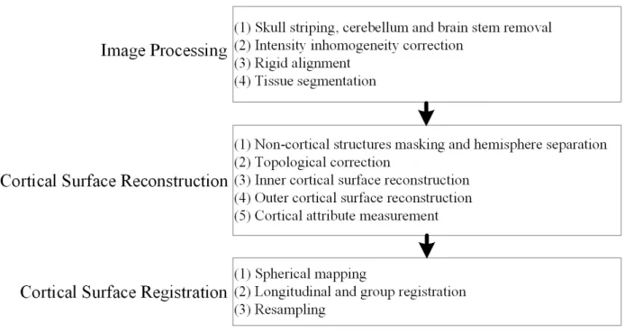
includes three main steps: image processing, cortical surface reconstruction, and cortical surface registration. Each step is introduced briefly next.
Figure 2.1. Data preprocessing pipeline.
2.2.1 Image Processing
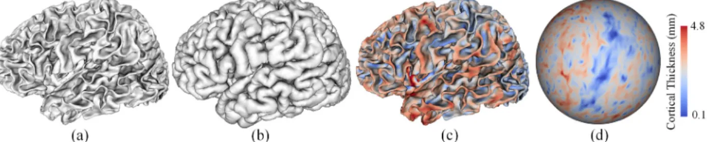
Figure 2.2. Examples of cortical surfaces and cortical thickness maps. (a) A reconstructed inner cortical surface. (b) A reconstructed outer cortical surface. (c)A cortical thickness map displayed on the corresponding inner cortical surface. (d) A cortical thickness map on the corresponding spherical surface.
2.2.2 Cortical Surface Reconstruction
was reduced to a location without such an intersection. For an infant with multiple scans at different ages, a longitudinal-consistent deformable model was used (Li, et al., 2014a; Li, et al., 2015b) to reconstruct the inner and outer cortical surfaces. Finally, the cortical attributes were measured. For example, cortical thickness of each vertex was computed as the mean of the minimum distances from the inner surface to the outer surface and also from the outer surface to inner surface (Li, et al., 2015a) as in FreeSurfer (Fischl, 2012). The sulcal depth of each vertex was defined as the shortest distance from the vertex to the cerebral hull surface, and was computed using the method in (Li, et al., 2014b). Some illustrative examples of the reconstructed cortical surfaces and cortical thickness maps are shown in Figure 2.1.
2.2.3 Cortical Surface Registration
stage, the average surfaces of all subjects were registered together and resampled, so the inter-subject vertex-wise correspondence was also established.
It is worth noting that, after the processing, all cortical attribute maps have also been mapped and resampled on the standard sphere. Figure 2.2(d) shows an example of a cortical thickness map on the resampled spherical surface.
2.3 Basis of Regression Forest
Random forest is a powerful machine learning tool, which has been widely used in the tasks of classification, regression, density estimation, and semi-supervised learning (Criminisi, et al., 2012). Since in this dissertation the random forest is used only for the regression, I will use the name “regression forest” instead of “random forest” in the rest of this dissertation. A regression forest consists of a number of binary decision trees that are trained independently. Each binary decision tree can recursively split the data into different subgroups according to predefined split functions, and at the end a regression value is computed for each subgroup. Each tree represents a “weak learner” with a limited ability of regression, but a linear combination of many “weak learners” as a forest yields an accurate regression result. It has also been discovered that grouping a set of randomly trained decision trees with slight differences could achieve higher accuracy on previously unseen data comparing than using a single over-trained decision tree, because of the generalization.
In the training stage, each decision tree in the forest is trained independently. To prevent over-fitting and increase generalization, usually each tree is trained using a subset of the whole training dataset. Given a set of training samples , | ∈ , ∈ , where and are respectively the d-dimensional feature vector and the scalar target value of the i-th training sample, each binary decision tree is trained by recursively finding a series of optimal partitions of the training samples. Specifically, at the root node, the training samples are optimally partitioned into two subsets by maximizing the following objective function:
arg max ,
| | | |
| |
| | (2.1)
where is the set of training samples at the current node; and are respectively the subsets of in the left child node and the right child node after the partition; is a metric that estimates the consistency of training samples in terms of regression target. Mathematically, is defined as:
| |∑ , ∈ (2.2)
where is the mean regression target value of all the training samples in . The partition is
determined by two factors and . For the -th sample in the training set, if the -th feature in
close to zero. For each leaf node, where the partition stops, a prediction model is used to compute the regression result based on all training samples falling into this leaf node. The prediction model could be in any form. The most popular prediction models includes (1) constant model, which averages the target values of training samples as the regression result, and (2) polynomial and linear model, such as ∑ .
In the testing stage, for each individual decision tree, the testing sample goes from the root node to a leaf node according to the results of binary tests in the non-leaf nodes, and the output is the regression result stored in the leaf node. The final result of the regression forest is the average of outputs from all decision trees.
2.3.2 Effects of Parameters
The performance of regression forest is affected by many factors. Next, I will briefly discuss some major factors, including the forest size, tree depth, weak learner model, and prediction model.
Forest Size. Forest size is the number of decision trees in a forest. Typically, increasing the number of trees would consequently make the prediction smoother and more stable. Such smoothness effect is stronger if the testing data moves away from the training data, which is a good thing for both interpolation and extrapolation. But larger number of trees also means more training and testing time. In practice, the forest size could be decided by gradually increasing the number of trees until the prediction errors stop changing.
training dataset. Increasing the depth would improve the fitting ability of regression forests. But a forest with too deep trees could yield over-fitting. In practice, there is often no lower bound limitation of the tree depth. The depth will keep increasing until it reaches the upper bound limitation. The upper bound limitation of the tree depth can be explicitly decided by a user-defined threshold, or can be implicitly decided by restricting the minimum sample size/information gain in the leaf node, which is a data-driven way.
Weak Learner Model. Weak learner model is the way of dispatching a training/testing
sample into left or right child node. The dispatching method introduced in Section 2.3.1 is an axis-aligned method, which partitions the feature space using an axis-axis-aligned hyperplane. General oriented hyperplane is another usually-used weak learner model. While the advanced weak learner model could strengthen the learning ability, it would also increase the computation complexity leading to longer training and testing time. Generally speaking, it is not always good to choose an advanced weak learner model, because stronger learning ability may somewhat reduce the variability of different trees and make the regression forest lose generalization. In practice, simple weak learner models are more preferred. Advanced models should be chosen carefully based on the priori knowledge about the dataset.
prediction model could be chosen based on the characteristics of the data distribution in the feature space.
2.3.3 Advantages and Disadvantages
Regression forest has many advantages over other regression methods, but also has some disadvantages. Both advantages and disadvantages will be briefly summarized in this section. Advantages
A few advantages of the regression forest are listed below.
1) Parallelization. Parallelization is an important factor to consider when selecting a machine learning algorithm. Because of the modern techniques of multi-core GPU and distributed computation system, a highly parallel algorithm always means higher computation ability and faster performance. As an ensemble model, each decision tree in a regression forest is trained independently, which makes regression forests easy to be parallelized.
2) Scalability. In the field of voxel-wise medical image analysis or vertex-wise surface-based analysis, the size of training data could easily reach millions, thus scalability is a very important factor when choosing a regression method. Due to the characteristics of binary decision tree, simply increasing the tree depth by one can double the capacity of a decision tree. In this way, regression forest can scale up efficiently. Moreover, the impact of such scaling up on the testing time is negligible, as only one layer is added in the tree.
in other forms, a regression forest could always fit the data without being provided explicit mathematical expressions. Second, the choices of weak learner models and prediction models are open to the users. They can use their prior knowledge about the dataset to design more specific models, and thus improve the overall performance. Disadvantages
There are two major limitations to keep aware of when using regression forest.
1) Storage. When using a massive training dataset with a large-scale and complex distribution, it could take a lot of space to store the trained regression forest. So in the case of limited hardware memory resource, regression forest may not be applicable. 2) Interpretability. Regression forests is not a descriptive tool. Though regression forest
could learn the relationship between the input features and the output regression value, the learned relationship is quite difficult to interpret. So, if the learning target is to find a descriptive relationship in the data, regression forest is not a good option.
2.4. Sulcal Pits
This section presents some background of the study of sulcal pits. I will first introduce the concept of sulcal pit and its important characteristics in Section 2.4.1, and then give an overview of the current research on sulcal pits in Section 2.4.2.
2.4.1 Sulcal Pit and Its Characteristics
controlled than the superficial parts (Le Goualher, et al., 1999; Le Guen, et al., 2017; Lohmann, et al., 1999; McKay, et al., 2013). Third, there are particular spatial relationships between the deepest parts of sulci and functional areas (Lohmann, et al., 2008; Piao, et al., 2004; Rakic, 1988; Smart and McSherry, 1986). Fourth, though the human cerebral cortex is highly variable across adult individuals, the spatial distribution of sulcal pits is relatively spatially consistent across human adult individuals (Im, et al., 2010; Lohmann, et al., 2008).
Because of these characteristics, sulcal pits have drawn increasing attention in neuroimaging studies in the past few years. A short review of the existing researches on sulcal pits is given in the next section.
Figure 2.3. Sulcal pits. Sulcal pits are displayed as small red balls. The cortical surface is color-coded by the value of sulcal depth.
2.4.2 Existing Research
small sizes. The results in (Im, et al., 2010) confirmed the observations in (Lohmann, et al., 2008), and further revealed the hemispheric asymmetries of sulcal pits. According to these studies, sulcal pits in major cortical sulci were considered as reliable anatomical landmarks and some of them could be potentially helpful for the challenging problem of inter-subject brain MR image registration. Im et al. (Im, et al., 2011a) further investigated the relationships between the presence of sulcal pits and intelligence, and found that in the left posterior inferior frontal sulcus and the right posterior inferior temporal sulcus, the number of sulcal pits of young adults with high IQ was significantly different from that of young adults with average IQ. McKay et al. (McKay et al., 2013) specifically studied the central sulcus in adults and found that most adult individuals had two peaks in the sulcal depth position profiles, close to the hand and mouth regions, where the peak genetic heritability of the sulcal depth occurred. By tracking the cortical surface development of four neonates between birth and four weeks of age (Lefevre et al., 2009), Lefèvre et al. found that the cortical surfaces grew in a radial manner from some “growth seeds”. Le Guen et al.
quantified the degree of how sulcal pits are under genetic controls in various brain regions (Le Guen, et al., 2017). Recently, sulcal pits have been applied to the study of psychological and neurological diseases, such as autism (Brun, et al., 2016), polymicrogyria (Im, et al., 2013b), and dyslexia (Im, et al., 2016).
2.5 Summary
3 ESTIMATION OF THE EARLY DEVELOPMENT OF CORTICAL ATTRIBUTES
Accurately modeling the development of cortical morphological attributes (cortical thickness, sulcal depth, etc.) is crucial for better understanding the mysterious dynamic early brain development and is also potentially helpful for the early diagnosis of neurodevelopmental disorders. This chapter focuses on the technical methods for estimating the early development of cortical attributes. To this end, two sub-problems are addressed in the chapter. Section 3.1 presents the techniques for addressing the first sub-problem, predicting the cortical attribute maps of future time points based on the known cortical attribute maps of the early time points. Section 3.2 presents the approach for addressing the second sub-problem, to approximately recover the missing cortical attribute maps in an incomplete dataset based on the available information. Finally, Section 3.3 summarizes the contributions in this chapter.
3.1 Predicting the Development of Vertex-wise Cortical Attributes
The rest of this subsection is organized as follows. First, some background and the motivation of DARF is introduced, and then the concept of DARF is introduced by illustrating the training and testing processes. Second, I will introduce how to extract surface-based Haar-like features from cortical attribute maps to support DARFs. Third, the proposed method is tested on an application of predicting the early development of cortical thickness maps, and the advantage of the proposed method is demonstrated by comparing with the existing popular techniques.
3.1.1 Dynamically-Assembled Regression Forest
Motivation
smooth as the real data, more than 90% of the area of an ROI needs to be overlapped with its neighboring ROIs. Unfortunately, such a large portion of overlap requires quite a large number of ROIs in order to cover the whole cortex, and thus leads to a large computational workload, as a respective set of individual trees need to be trained for each ROI. Taking account of all these issues, I propose a Dynamically-Assembled Regression Forest (DARF). By first training a single decision tree for each vertex in the training stage and then locally grouping decision trees of neighboring vertices as forests in the testing stage, DARF is able to produce spatially smooth regression results and meanwhile also save a lot of computational cost.
Training Stage
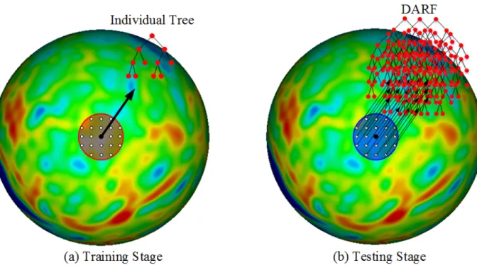
In the training stage, one individual binary decision tree is trained at each vertex on the cortical surface. As shown in Figure 3.1, for the given vertex on the spherical cortical surface (mapped from the original cortical surface), one individual tree is trained using the nearby vertices within a training-neighborhood (i.e., the red region) as training samples. Each training sample can
be denoted as a pair of a feature vector and a scalar regression target ∈ , ∈ . The feature vector consists of a set of features extracted from the local cortical attribute maps around the vertex at the input time point(s) (see Section 3.1.2), and the scalar target is the cortical attribute value of vertex at the target time point.
Testing Stage
result is finally computed as the average of regression outputs from all trees of the formed forest. Of note, the optimal size of testing-neighborhood can be learned via a cross validation.
Figure 3.1. Training and testing stages for DARF. (a) The red region is the training neighborhood, where all the vertices on the spherical space are used as training samples. (b) The blue region is the testing neighborhood, where all the individual trees are combined together to form a forest in the testing stage. Note that the red and blue regions in (a) and (b) could have different sizes.
Different from the original way of using a regression forest, which trains a set of trees and makes them a fixed forest at the training stage, our method does not assign trees to any forest in the training stage. Instead, the forest is formed by group neighboring trees during the testing stage, and thus it is named “Dynamically-Assembled” Regression Forest. This novel way of forming forest has two advantages.
local cortical attribute maps, are also similar. By feeding the similar input features to the similar DARFs, the outputs at neighboring vertices generally have small differences, and thus the predicted cortical attribute map is smooth.
The second advantage is that, since one single decision tree can be shared by many nearby forests, the computational cost for training forests is significantly reduced. For instance, if in each forest there are 100 trees, using DARF would save 99% computational cost compared to the case of using the original regression forests (i.e., training a forest at each vertex). Even compared to the ROI-based strategy, DARF still significantly saves the computational cost in the training stage. Based on my experiments, to achieve the smooth predicted cortical attribute maps, highly-overlapped ROIs are needed, with the number of ROIs being nearly 20% of the number of vertices. If each forest owns 100 trees, using DARF would still save 19% computational cost.
3.1.2 Input Features
Figure 3.2. Computation of Haar-like features on a resampled spherical surface atlas. The blocks
A and B are the two randomly selected regions. The value of Haar-like feature is defined as 1) the mean value of the cortical attributes in the block A, or 2) the mean value of the cortical attributes in the block A subtracting that in the block B.
Figure 3.2 illustrates how to compute context features from a local cortical thickness map for a vertex on the resampled sphere. Assuming now we are training a decision tree at the vertex , and without loss of generality ( could be equal to ), we assume vertex is a neighbor of vertex .
The local cortical thickness map around the vertex is projected onto the tangential plane, where a local 2D coordinate system is built at the center of the vertex , and ′ is the projection of vertex on the tangential plane. Two blocks and are randomly selected in the neighborhood , , with their sizes and chosen randomly within the interval , ,
where , , , and are the user-defined parameters. Letting denote the set of all vertices in block and denote the set of all vertices in block , the context feature at vertex can be defined as:
where , is the value of cortical thickness at position , , and is a random coefficient that takes either 0 or 1.
3.1.3 Quantitative Evaluation
To quantitatively evaluate the estimation results, we employed three metrics: NMSE (normalized mean squared error) (Faramarzi, et al., 2013), MAE (mean absolute error), and MRE (mean relative error). These metrics are respectively computed as follows:
∑
∑ (3.2) ∑ | | (3.3)
∑ (3.4)
where and are respectively the ground truth and the estimated result, and is the number of vertices.
3.1.4 Experiments and Results
loops were used. The inner cross-validation loop was used to tune the parameters of DARF, while the outer loop leave-one-out cross validation was used to evaluate the prediction results.
Individual-level Inspection
For each individual, the predicted cortical thickness map was compared with its ground truth, which was obtained using the method in Section 2.2.2, and the prediction error map was computed. Figure 3.3 provides an example of the predicted cortical thickness maps based on the data at 1 month of age for a randomly selected subject. It is clear that the predicted map is generally quite similar to the ground truth.
Figure 3.3. Prediction of the cortical thickness maps for a randomly selected subject. Group-level Inspection
subjects. As shown in Figure 3.4, the distribution of the predicted cortical thickness is generally similar to the distribution of ground-truth cortical thickness.
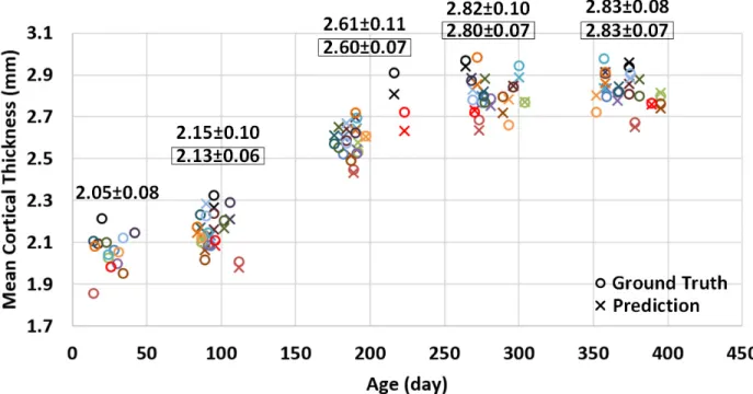
Figure 3.4. Predicted mean cortical thickness and ground truth. This figure plots the longitudinal distribution of ground-truth mean cortical thickness and its corresponding prediction (over the whole cortical surface) for 15 subjects. Different subjects are distinguished by different colors. For each time point, the average ground-truth mean cortical thickness over all 15 subjects and standard deviation are provided on the top of data distribution, and the values within each black rectangle denote the average and standard deviation of the corresponding prediction results.
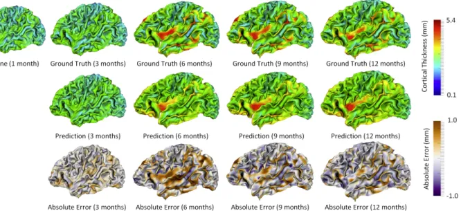
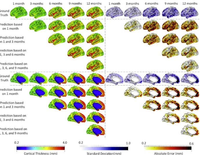
time points for prediction would generally achieve better results. Additionally, we can see that the error map at each time point is highly correlated with the corresponding standard deviation map of cortical thickness across individuals, with the averaged correlation coefficient of 0.8±0.05. Another observation based on Figure 3.5 is that the standard deviations at the 6th and 9th months are relatively larger than those at other time points, and accordingly the prediction errors at the 6th and 9th months are also larger compared with other time points. Of note, the large standard deviation of cortical thickness estimation errors at the 6th and 9th months might be caused by the extremely low tissue contrast of infant MRI at these ages, which makes both cortical surface reconstruction and measurement more challenging and less accurate. In Figure 3.5, we can also observe that the prediction accuracy peaks in the unimodal cortex, e.g., the precentral gyrus (primary sensory cortex), postcentral gyrus (primary motor cortex) and occipital cortex (visual cortex), while the prediction accuracy drops in the high-order association cortex, e.g., the prefrontal cortex, temporal cortex, insula cortex, and inferior parietal cortex.
Figure 3.5. The prediction results from multiple available time points, averaged across 15 subjects. The 1st row and the 6th row show, respectively, the averaged cortical thickness maps (left half columns) and corresponding standard deviation maps (right half columns) at all 5 time points. The 2nd–5th rows and the 7th–10th rows show the predicted cortical thickness maps (left half columns) and the corresponding error maps (right half columns).
Table 3.1. Quantitative measures of cortical thickness prediction using mean absolute errors (MAE).
MAE (mm) Target Time Point
Table 3.2. Quantitative measures of cortical thickness prediction using mean relative errors (MRE).
MRE (%) Target Time Point
Used Time Point(s) 3rd month 6th month 9th month 12th month
1st month 9.9±1.1 13.1±0.9 12.4±0.8 11.7±0.9
1st, 3rd months - 12.3±0.8 11.7±0.7 11.0±0.7 1st, 3rd, 6th months - - 9.5±0.8 9.0±0.7 1st, 3rd, 6th, 9th months - - - 7.9±0.6
Region-based Evaluation
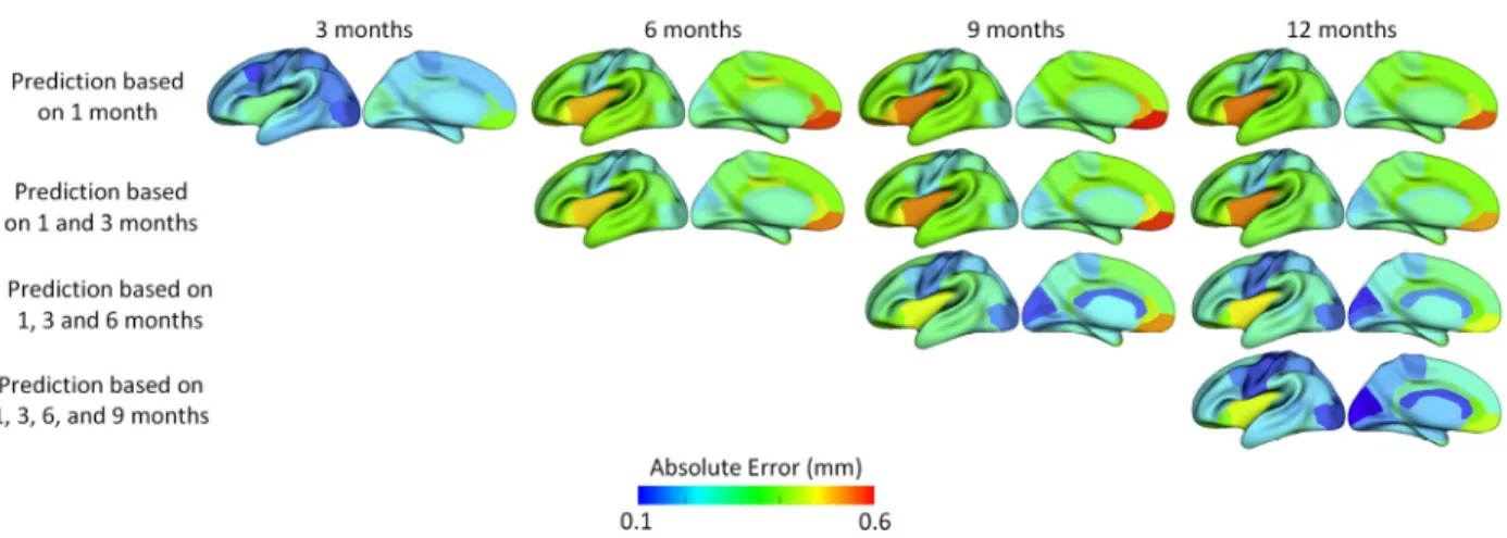
I parcellated each cortical surface into 35 regions using the method developed in (Li, et al., 2014c), and then computed the average prediction error in each region. As shown in Figure 3.6, the regions with smaller errors generally included the unimodal cortex, such as the sensorimotor region (precentral gyrus and postcentral gyrus) and visual area (including cuneus cortex, pericalcarine cortex, lingual gyrus, and lateral occipital cortex), while the regions with larger prediction errors represented the high-order association cortex, such as the prefrontal, lateral temporal, cingulate, and insula cortices.
Figure 3.6. The average prediction errors (mm) in 35 cortical ROIs for 15 infants.
Comparison with Other Methods.
(SLR). MEM, which explicitly models fixed effects and random effects, is a powerful method for analyzing longitudinal neuroimaging data. In our comparison experiments, MEM assumes that the development of cortical thickness increases with age (fixed effect) during the first year, while each subject has individual variations (random effect), such as genetic and environmental influences. PR method assumes that the development of cortical thickness at each vertex has a second-order polynomial relationship with age. CRF trains a single forest for the entire surface with the spherical location of each vertex as additional features (in addition to the Haar-like features). SLR is an effective method for high-dimensional data analysis (Tibshirani, 1996), which can extract the most “useful” features from a high-dimensional feature representation by setting zero coefficients for irrelevant features. Specifically, given a target vector , , … , ∈ and the feature
matrix , , … ∈ , SLR method finds the optimal coefficients , , … ∈ by solving the equation below:
arg min
∈ ‖ ‖ ‖ ‖ (3.5)
where and were optimally set to 12 and 0.001 respectively in our experiments based on a grid search, which was performed on a subset of the training data.
Figure 3.7 provides a comparison among MEM, PR, CRF, SLR and DARF for predicting
Figure 3.7. Prediction of the vertex-wise cortical thickness map (mm) of a randomly selected infant at 9 months of age by five different methods. The first row shows the ground truth and the estimated thickness maps by five different methods. The second row shows the estimation error maps (mm), along with the zoomed-up ROIs.
3.2 Estimating the Missing Cortical Attribute Maps
This section presents the techniques of how to make a better use of the available data in an incomplete longitudinal dataset to estimate the missing data. Section 3.2.1 introduces the approach in detail. Section 3.2.2 describes all the evaluations and comparison experiments and reports the results.
3.2.1 Missing Cortical Attribute Estimation Method Motivation
of training subjects and engaging more time points are conflicting with each other. For example, as shown in Figure 3.8, to estimate the missing data at 6 months of age, I can use at most 28 subjects to train the regression model, since 28 infants have real data at both 1 and 6 months of age. Consequently, only 1 time point (i.e., at 1 month of age) is taken account into the training process. In another way, I can engage at most 4 time points in the training process, but only 16 infants have real data at all 5 time-points and can be used as training subjects. To eliminate this confliction and fully utilize the available information, a two-stage missing data estimation strategy is proposed. Figure 3.9 shows the overview of the proposed strategy, containing the stages of 1) pairwise estimation and 2) joint refinement.
Figure 3.8. Illustration of the longitudinal infant dataset used in this study. Each block indicates the cortical morphological attributes of all vertices of the entire cortical surface for a specific subject (column) at a specific time point (row). The black blocks indicate the missing data at the respective time point. The blocks enclosed by the red rectangle indicate the dataset used in this dissertation.
training subjects to train a set of decision trees. During the training, the data at 6 months of age is the regression target and the data at 1 month of age are the inputs. After training, for the subjects with available data at 1 month of age but without data at 6 months of age, these decision trees are dynamically/locally assembled as the forest to estimate the missing data at 6 months of age. Similarly, the estimations of missing data at 6 months of age can be obtained, respectively, using the existing data at each of the 3, 9, and 12 months of age. In this way, the available data at all other time points can contribute to the estimation of the data at 6 months of age. Finally, all the estimations contributed from different time points are averaged together as the initial estimation. Similarly, for the missing data at each of 1, 3, 9, and 12 months of age, the same process can be performed to obtain their initial estimations. After performing Stage 1, the missing data of all subjects at all time points will be approximately recovered, thus providing a pseudo-complete longitudinal dataset.
Figure 3.9. Overview of the missing data estimation method. The box with number stands for the data at the corresponding time point. The directed edges represent the processes of estimating the missing data at the target time points (as pointed by the arrowhead) based on the data at the available time points (at the tail side). In Stage 1, the edges are bidirectional, which means that the estimation is performed twice by exchanging between the input and the output time points. The circles in Stage 2 denote the use of multiple time points jointly.
the data at all other time points jointly. For example, to obtain the final estimation of the missing data at 6 months of age, all subjects with real data at 6 months of age are used as the training subjects to train a set of decision trees. During the training, the data at 6 months of age is the regression target and the data at 1, 3, 9, and 12 months of age are the inputs. After training, for each subject with missing data at 6 months of age, the trained decision trees can be dynamically/locally assembled as the forest to estimate the missing data. Note that it is not required that each training/testing subject must have real data at 1, 3, 9, and 12 months of age, since the missing data have already been recovered in Stage 1. Similarly, for the missing data at other time points, the same process can be conducted to obtain their final estimations. It is worth noting that, using the above two stages (Stage 1 and Stage 2), the proposed strategy can effectively leverage the information from all time points of all available training subjects for the missing data estimation.
3.2.2 Experiments and Results
Figure 3.10. Estimations of the vertex-wise missing cortical thickness at 9 months of age for a randomly-selected infant. The first two columns show the maps of ground truth and the estimated cortical thickness at each step. The last two columns show the maps of estimation errors at each stage.
further shows the averaged errors for all reference subjects in each step of estimation. From these two figures, we can see that using the data at 6 or 12 months of age as inputs to estimate the cortical thickness at 9 months of age is better than the case of using the data at 1 or 3 months of age. A possible explanation is that the cortical thickness at 9 months of age is more similar to cortical thickness at 6 and 12 months of age, compared to cortical thickness at 1 and 3 months of age. Figure 3.11 also shows that the result of joint refinement is generally better than all the results in the previous stage (Stage 1), indicating the effectiveness of joint refinement stage (Stage 2). Figure 3.12 illustrates the average estimation errors of vertex-wise cortical thickness at all 5 time points.
Figure 3.12. Average vertex-wise errors (mm) in estimating the missing cortical thickness at 5 time points for all subjects by using the proposed method.