Vol 2, No 4 (2016)

JEEECCS, Volume 2, Issue 6, pages 9-14, 2016

Solutions for Driving 2DW/1FW Mobile

Robots using Sliding-Mode Control

Henri-George COANDĂ, Electrical Engineering, Electronics, and

Information Technology Faculty “Valahia” University of Targoviste

Targoviste, Romania

[email protected]

Eugenia MINCĂ, Ion CĂCIULĂ, Florian ION Electrical Engineering, Electronics, and

Information Technology Faculty “Valahia” University of Targoviste

Targoviste, Romania

Abstract – In this paper the behaviour of one mobile robot 2DW/1FW using sliding-mode control is analysed. An algorithm developed in Stage to achieve this result was used. Mapper3 is used for map design and the MobileSim environment is used for simulation. The robot used in this paper is Pioneer P3-DX, produced by Adept Mobile Robots. The analyses are focused on the behaviours of the robot according to certain parameters.

Keywords - mobile robots, Pioneer P3-DX, ARIA, MobileSim, Mapper3, sliding-mode

I. INTRODUCTION

The sliding-mode control is recognized as an effective method for achieving robust control with high-fidelity, for nonlinear systems, also under dynamic conditions and in an unsafe environment. The researches in this field began 40 years ago and are still receiving enough attention from the international scientific community in the past two decades. Some of the relevant results to that field are presented in [1]- [4], highlighting the presence of this subject over the years.

The major advantage of the sliding-mode control is the way to reduce sensitivity parameter variations and disturbances, leading to elimination of the need of an accurate model. The control law defined follows the system trajectory inside two surfaces named switching surfaces.

The sliding-mode controller is based on a closed loop, which offers switching at high frequencies. The great advantage is robustness to variation of parameters and control disturbances, and the main problem lies in the trepidation phenomenon, whose reduction is pursued. Using sliding-mode, system behaves as a low-order system compared to the whole process and the switching over sliding surfaces does not suffer changing due to model changes or disturbances.

II. MOBILE PLATFORM - PIONEER P3-DX

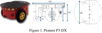
The mobile platform Pioneer P3-DX (Figure 1) is part of a family of mobile robots produced by the company Mobile Robots. This family also includes AT Pioneer, Pioneer 2-DX, and many others. These

mobile development platforms have in common the software architecture and can be equipped with 2 or 4 wheels for driving.

Figure 1. Pioneer P3-DX

The Pioneer P3-DX is equipped with on-board management system, thus becoming an autonomous mobile robot. Unlike other robots, Pioneer P3-DX is a mobile platform with small size, allowing navigation on the narrow aisles and on crowded spaces. The management system of the robot Pioneer 3-DX uses two DC motors, each equipped with a high resolution optical encoder for precise positioning and high sensitivity to determine the speed.

The Pioneer P3-DX can climb with uphill gradient of up to 25% and on ground level the mobile robot speed can reach up to 1.6 m/s (5.76 km/h). Its weight is 9 kg with a minimum number of batteries. These features enable it to carry a load of up to 23kg. The mobile robot is equipped with front end sonar. The 8 sensors have an operating range between 15cm and 5m.

Of the eight sensors, two are on the left and right sides and the other six in front, being situated in a range that covers an area of 15 degrees. Optionally, the robot can also have a ring of sonar in the back, with the same configuration. On the control side, there are an embedded PC/104 computer and I/O modules connecting various external devices.

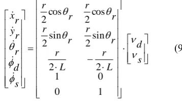
III. THE KINEMATIC MODEL

It is assumed that the vehicle's wheels rotate without slipping, so the robot is subject to non-holonomic constraints described by the equation:

 A(q)q0 

where A(q) is the matrix associated to the constraints.

Figure 2. Kinematic model for Pioneer P3-DX

For the mobile robot in Figure 2, Oxy is the coordinate system,

CPX

_r

Y

_ris attached to the robot coordinate system, the distance between CP and the centre of gravity is d and CP is midway between the two wheels. In this case the constraints are:

 y_rcos



_rx_rsin



_rd



0 

 x_rcos_r y_rsin_r LR_d 

 s R L r r y r r

x cos  sin      The matrix A(q) becomes:

                r b r r r b r r d r r q A 0 sin cos 0 sin cos 0 0 cos sin ) (        

In this case, the configuration of the robot is represented using five generalized variables



y_{r r r l}



r x

q    _{, where the coordinates of CP}

are





r y r x , ,

r

 is the orientation, and _d,_s are the driving wheel’s angles.

Let us consider the matrix S(q) such that:

 ST(q)AT(q)0  i.e., one in relationship (7):

















                                        1 0 0 1 2 2 cos sin 2 cos sin 2 sin cos 2 sin cos 2 ) ( L r L r r d r L L r r d r L L r r d r L L r r d r L L r q S         

The kinematic model of the robot becomes:

 qS(q) 

where [ ]

s d  

  represents the angular speeds of

the drive wheels. Eq. (8) is written as:

                                                      s d L r L r r r r r r r r r s d r r y r x          1 0 0 1 2 2 sin 2 sin 2 cos 2 cos 2       

The relationship between the linear velocity and the angular velocity and the angular speeds of the driving wheels is written as:

                             r r v r r r L r s d    1 1 1  

By replacing Eq. (10) into (9), the kinematic model is simplified as follows:

                                 r r v r r r r y r x   

 0 1 0 sin 0 cos      where: r

x - is the position of the robot on Ox axis

r

y - is the position of the robot on Oy axis

r

 - is the robot orientation

r

v - is the linear velocity of the robot

r

 - is the rotational speed of the robot.

The kinematic models describing the movement of the robot or vehicle do not take into account the forces acting on them and are used to calculate the command for driving WMR.

To obtain the kinematic model for WMR, the generalised variables for the system, as well as rotation of the wheels without slip, are considered. In addition, the non-holonomic constraints are applied to the robot. The result of the model has five variables: two variables for the geometric centre of WMR, a variable for steering angle of the robot and other two variables representing angle for each wheel. These variables depend on the speed of rotation of the wheels. The model is simplified because the authors’ intention was to find the Cartesian coordinates of the geometric centre and the steering angle by replacing the speed of the two wheels with the linear velocity and the angular velocity of the robot.

IV. DESIGNDRIVINGSTRUCTUREOF

SLIDING-MODE

The trajectory tracking problem involves designing a controller to calculate the linear velocity and angular velocity and to enable the real vehicle to follow the path of the virtual vehicle with small positioning errors.

Figure 3. Sliding-mode controller

The virtual kinematic model of the vehicle was presented in Section III, and the last relation was:

            d d d d v d y d d v d x        sin cos  

where ( , )

d y d

x are the Cartesian coordinates for the

geometric centre, v_d is the linear velocity, _d is the

orientation, and _d is the rotational speed. The tracking errors are:

                                     d r d y r y d x r x d d d d e e y e x      

 0 0 1 0 cos sin 0 sin cos  

The dynamic tracking error is:

                   d r e e x d e r v e y e y d e r v d v e x           sin cos  

The tracking errors described in Eq. (13) are shown in Figure 4. Considering tracking errors and their derivative Eq. (14) the switching surfaces are defined as follows:

 s₁x_ek₁x_e   s₂y_ek₂y_ek₀sign(y_e)



_e 

The control law is used in the following form:

 ̇ ( )  

Figure 4. Tracking errors for mobile robots

The sliding-mode control law is obtained from the following two relationships:

) 1 1 1 ) 1 ( 1 ( cos 1 e x k s P s sign Q e c

v       

 ) ( cos 1 e y d e y d e         

 ( sin )

cos 1 d v e e r v e   _{ }        ) sgn( 0 cos sin 2 2 2 ) 2 ( 2 e y k e r v e c v e y k s P s sign Q

c _{  }

               d e y k e r v e x d e x d _             ) sgn( 0 cos    

Let V  sT s

2 1

be a Lyapunov function.

The derivative of this function is:



) _{1 1}



1 sgn( 1 1 2 2 1

1 s s s s Q s P s

s

V         

 s₂



Q₂sgn(s₂)P₂s₂



 

The Lyapunov function derivative is semi-defined negative if the parameters Q_i,P_i 0 are considered.

V. SOFTWAREARCHITECTURE

The analysis was performed using MobilSim [7] software from Mobile Robots - software for simulation into MobileRobots / ActivMedia platforms and their environments and experimentation with ARIA [8]. MobileSim replaces SRISim that was previously distributed with ARIA. MobileSim is based on the Stage simulator, created by Richard Vaughan, Andrew Howard and others as a part of the project Player / Stage, with some modifications from MobileRobots. MobileSim can simulate the behaviour of all robots produced by MobileRobots. A map in Mapper3basic is created for simulation and further loaded in MobileSim. The programs are written in C++ and compiled in Visual Studio. Communication with the simulator is realised using ARIA functions.

Figure 5 presents the two options used by the authors. In the simulation Mapper3, ARIA, Visual C++ and MobileSim are used, and in real tests, ARIA, Visual C++, USR VCOM and Pioneer P3-DX are used as well.

VI. RESULTS

The controller proposed for driving the WMR 2DW/1FW robot was tested in the simulation environment with MobileSim software from Mobile Robots and in the real environment, respectively. The program was written in C++ and can run on a laptop with sampling frequency of 100ms. To validate the proposed methods, the real-time simulations and tests are described below. The ARIA functions setVel(Velocity), setRotVel(Angular Velocity), and setVel2(leftVelocity, RightVelocity) are used here for sending the commands computed by dedicated procedures. They read data from the robot together using ARIA: getX(), getY(), getTH(), getRotVel(), getVel().

The first test was aimed at obtaining a linear trajectory with a speed of 0.5 m/s by the 2DW / 1FW vehicle using continuous sliding-mode algorithm (10 m, 20 s). The results in real environment are drawn with the red continuous line as shown in the following figures. Figure 6 presents the trajectory resulting from driving using sliding-mode in continuously time. Figure 7 shows the orientation error of the robot when driving using sliding-mode, while Figure 8 shows the error on the X axis. Figure 9 shows the error on the y-axis all generated by sliding-mode controller. Figure 10 presents the sliding surface s1, and Figure 11 shows the sliding surface s2 calculated in driving sliding-mode.

Figure 6. Trajectory – 1st _test

Figure 7. Error tracking direction – 1st test

Figure 8. X-axis tracking error – 1st _test

Figure 9. Y-axis tracking error – 1st _test

Figure 10. Sliding surface s1 – 1st test

It is observed that the positioning errors are small in the first linear 10m and 20s, the performance tracking trajectory is pretty good when using sliding-mode for WME 2DW/1FW. The following values are used here: Q1=0.05, Q2=0.5, P1=0.5, P2=0.75 for the control law, k0=30, k1=0.75, k2=25 for switching surfaces, vd = 0.5m/s, 200 iterations straight (w=d=d’=0).

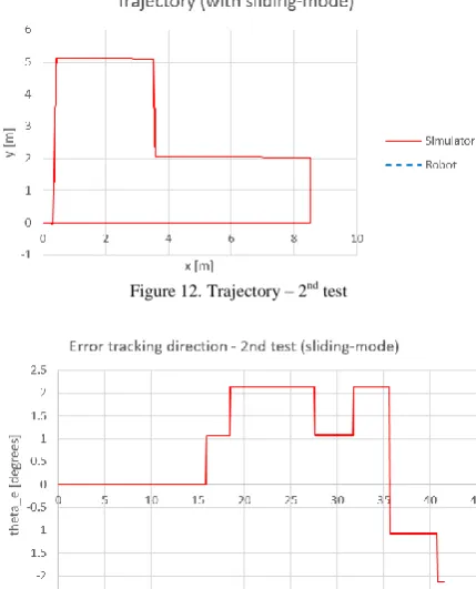
In the second test, a imposed route is considered, corresponding to a production line by vehicle 2DW / 1FW using sliding-mode (13 straights scroll). Sliding-mode control is repeated for each segment of the route. The cumulative effect for the whole route is observed in the image.

Figure 12 depicts the trajectory resulting from driving using sliding-mode in continuous time. Figure 13 shows the orientation error of the robot when driving using sliding-mode. Figure 14 presents the sliding surface s1 and Figure 15 shows the sliding surface s2 calculated driving sliding-mode.

Figure 12. Trajectory – 2nd _test

Figure 13. Error tracking direction – 2nd _test

The following values are used here: Q1=0.05, Q2=0.5, P1=0.5, P2=0.75 for the control law, k0=30, k1=0.75, k2=25 for switching surfaces, vd = 0.5m/s, 200 iterations straight (w=d=d’=0).

Figure 14. Sliding surface s1 – 2nd _test

Figure 15. Sliding surface s2 – 2nd _test

Figure 13 shows the changes of direction with 900, 1800, 900, 1800, 2700 and 1800 (transitions) and the very small tracking errors using sliding-mode on the straight lines (landing). Figures 14 and 15 show the sliding-mode control applied after each turning point and after each stop next to a workstation. The effect of the integration block is observed in Figure 3.

VII. CONCLUSION

In this paper, the behaviour of the robot in a real environment according to a map of coordinates has been analysed. Furthermore, its behaviour when driving based on sliding mode control has been simulated and tested.

The algorithms have been developed by using Visual C++ environment and ARIA Stage library. The Mapper3 program has been used for developing the maps, and MobileSim has been used as simulator. The results of the tests have demonstrated that the model parameters of sliding-mode controller can affect the errors. Additionally, the results of the tests are useful to identify the values that lead to a minimum of errors.

ACKNOWLEDGMENT

REFERENCES

[1] W Gao, JC Hung, Variable structure control of nonlinear systems: a new approach, IEEE Transactions on Industrial Electronics, Vol. 40, No. 1, pp. 45-55, Feb 1993.

[2] Giorgio Bartolini, Leonid Fridman, Alessandro Pisano, Elio Usai, Modern Sliding Mode Control Theory - New Perspectives and Applications, Springer, ISBN 978-3-540-79016-7, 2008.

[3] Vadim Utkin, Jurgen Guldner, Jingxin Shi, Sliding Mode Control in Electro-Mechanical Systems, Automation and Control Engineering Series, CRC Press, ISBN 978-1-4200-6560-2, 2009.

[4] A Şabanoviç, Variable structure systems with sliding modes in motion control-a survey, IEEE Transactions on Industrial Informatics, Vol. 7, No. 2, pp. 212-223, pp. 212-223, 2011. [5] Solea R., Sliding mode control applied in trajectory-tracking

of WMRs and autonomous vehicles, PhD Thesis, University of Coimbra, Portugal, 2009.

[6] Bogdan Dumitrașcu, Contribuţii la conducerea, navigaţia şi evitarea de obstacole a roboţilor mobili şi vehiculelor autonome (in Romanian), Universitatea “Dunărea de Jos din Galați”, PhD Thesis, 2012.

[7] G Petrea, A Filipescu, A Filipescu, R Solea, S Filipescu, Visual servoing and sliding-mode controller for a mobile robotic system integrated in a processing/reprocessing mechatronics line, 2015

http://www.prorobsis.ugal.ro/published_papers.html [8] Filipescu, A., Minca E., Voda A., Dumitrascu B., Filipescu

A., Jr., Ciubucciu G., Sliding-Mode Control and Sonnar Based Bubble Rebound Obstacle Avoidance for a WMR, Proceedings of the 19th IEEE, International Conference on System Theory, Control and Computing, ICSTCC 2015 14-16, Oct. Cheile Gradistei, Romania, 2015, pp.105-110, ISBN: 978-1-4799-8481-7, 2015

[9] Amanda Whitbrook, Programming Mobile Robots with Aria and Player, Springer-Verlag London Limited, 2000. [10] MobileRobots, Advanced Robotics Interface for Applications