Volume 29: Graph Transformation and Visual Modeling Techniques 2010

(1)

Proceedings of the

Ninth International Workshop on

Graph Transformation and

Visual Modeling Techniques

(GT-VMT 2010)

A lightweight abstract machine for interaction nets

Abubakar Hassan, Ian Mackie and Shinya Sato

12 pages

Guest Editors: Jochen K ¨uster, Emilio Tuosto

Managing Editors: Tiziana Margaria, Julia Padberg, Gabriele Taentzer

(2)

A lightweight abstract machine for interaction nets

Abubakar Hassan1, Ian Mackie2and Shinya Sato3

1_{Department of Informatics, University of Sussex, Falmer, Brighton BN1 9QJ, UK}

2_{LIX, CNRS UMR 7161, ´}_{Ecole Polytechnique, 91128 Palaiseau Cedex, France}

3_{Himeji Dokkyo University, Faculty of Econoinformatics, 7-2-1 Kamiohno, Himeji-shi, Hyogo}

670-8524, Japan

Abstract: We present a new abstract machine for interaction nets and demonstrate that an implementation based on the ideas is significantly more efficient than existing interaction net evaluators. The machine, which is founded on a chemical abstract machine formulation of interaction nets, is a simplification of a previous abstract machine for interaction nets. This machine, together with an implementation, is at the heart of current work on using interaction nets as a new foundation as an intermediate language for compiler technology.

Keywords:Interaction nets, programming languages, abstract machine

1 Introduction

Interaction nets [Laf90] are a graphical model of computation. It is possible to program with interaction nets [HMS09, Mac05] and they also serve as an intermediate language for imple-menting other programming languages. Some examples are encodings ofλ-calculus, and simple

functional programming languages (amongst others, see for instance [AG98,GAL92,Mac98]). One reason why they have been very successful at implementing other programming lan-guages is that a compilation must explain all the components of a computation. What is rare, is that the compilation can give something back, and this has been observed with the encodings on theλ-calculus where new strategies for reduction have been found. One of the reasons for this is because interaction nets naturally capture sharing, indeed one has to work hard to simulate reduction strategies where duplication of work takes place.

In [FM99] a calculus was given which provided a foundation for the operational understanding of interaction nets. This calculus led to the development of an abstract machine [Pin00], which in turn led to a very efficient implementation of interaction nets.

Recently, there have been new developments in the foundations for a calculus of interaction nets. The purpose of this paper is to outline these ideas which led to the main contribution of the paper which is an abstract machine founded on the new calculus. This in turn has led to the development of new implementations of interaction nets which are the most efficient that we are aware of to date.

(3)

developed.

The main contributions of this paper are:

• We define a new term calculus of interaction nets. The novelty is that the notion of substi-tution is simplified in that it just replaces a name.

• We simplify and improve Pinto’s abstract machine [Pin00] by using this calculus. The main improvement is due to the fact that we no longer need to maintain lists of names, and consequently the transition rules become significantly more simple.

• We have built a prototype implementation based on the ideas. We demonstrate that we get a factor of ten improvement over previous implementations, and this implementation is thus the most efficient evaluator to date.

Overview. The rest of this paper is structured as follows. In the next section we review what we need about interaction nets. In Section 3 we give our new calculus. Section 4 gives the abstract machine, and gives studied properties of it. We conclude the paper in Section 5.

2 Interaction nets

Here we review the basic notions of interaction nets. We refer the reader to [Laf90] for a more detailed presentation. Interaction nets are specified by the following data:

• A set Σof symbols. Elements of Σ serve as agent (node) labels. Each symbol has an associated arity ar that determines the number of its auxiliary ports. If ar(α) =n for α∈Σ, thenαhasn+1ports: nauxiliary ports and a distinguished one called theprincipal

port.

… x1 xn

ë

• Anetbuilt onΣis an undirected graph with agents at the vertices. The edges of the net connect agents together at the ports such that there is only one edge at every port. A port which is not connected is called afree port. A set of free ports is called aninterface.

• Two agents(α,β)∈Σ×Σconnected via their principal ports form anactive pair (analo-gous to a redex). An interaction rule((α,β)−→N)∈Rin replaces the pair(α,β)by the netN. All the free ports are preserved during reduction, and there is at most one rule for each pair of agents. The following diagram illustrates the idea, whereNis any net built fromΣ.

…ì …ì x1 xn y1 ym

N

… …

x1 xn y1 ym

(4)

S

add add

S

r y x

r

y x

Z

add

r y r y

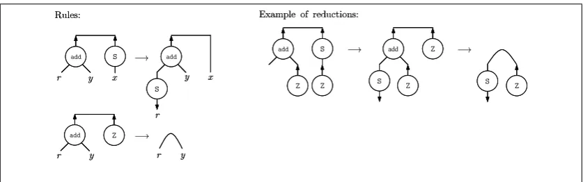
Rules: add add Z Z S Z Z

S S _Z

Example of reductions:

SS

add

add addadd

SS

r y x

r

y x

ZZ

add add

r y r y

Rules:

add

add addadd

ZZ ZZ SS

ZZ ZZ

SS SS _ZZ

Example of reductions:

Figure 1: An example of a system of interaction nets

We use the relation−→for the one step reduction and−→∗for its transitive and reflexive closure. Interaction nets have the following property [Laf90]:

Proposition 1(Strong Confluence) Let N be a net. If N −→N1 and N−→N2with N16=N2,

then there is a net N₃such that N₁−→N₃and N₂−→N₃.

Figure 1 shows a classical example of an interaction net system that encodes the addition operation. We can represent numbers using the agents S to represent the successor function (n7→n+1)andZto represent the number 0. The left of the figure contains the two addition rules which we leave the reader to relate to the standard equational term rewriting system definition of addition. The right of the figure gives an example reduction sequence which shows how a net representing 0+1 is reduced to 1 using the given rules.

2.1 The calculus for interaction nets

In this section we review the calculus for interaction nets proposed by Fern´andez and Mackie [FM99]. We begin by introducing a number of syntactic categories:

Names LetN be a set ofnamesranged over byx,y,z,x₁,x₂, . . .. We write ¯x,y¯, . . .for sequences of names. We assumeN andΣare disjoint.

Terms are built fromΣandN using the grammar: t::=x | α(t1, . . . ,tn), wheret1, . . . ,tnare terms,α∈Σandar(α) =n. Ifar(α) =0, then we omit brackets and write justα. We use

t,s,u, . . .to range over terms and ¯t,s¯,u¯, . . .over sequences of terms.

Equations have the form: t=s, wheretandsare terms. Equations are elements of computa-tion. Given ¯t=t₁, . . . ,tkand ¯s=s1, . . . ,sk, we write ¯t=s¯to denote the listt1=s1, . . . ,tk=

sk. We use∆,Θ, . . .to range over multisets of equations.

(5)

Interaction rules have the form: α(t1, ...,tn)onβ(s1, ...,sk), whereα(t1, ...,tn)andβ(s1, ...,sk)

are terms. This notation for rules was introduced by Lafont [Laf90] and we refer to it as Lafont’s style. All names occur exactly twice in a rule, and there should be at most one rule between any pair of agents inR. R is closed under symmetry, thus ifα(t¯)onβ(s¯)∈R

thenβ(s¯)onα(¯t)∈R.

Definition 1(Bound names) If a namexoccurs twice in a termt, then we sayxisbound. We extend this notion to equations, sequences of terms, and multiset of equations.

The calculus consists of three reduction rules which reduce (valid) configurations.

Indirection:

ht¯|x=t,u=s,∆i−→iht¯|u[t/x] =s,∆i wherexoccurs inu,

Collect:

ht¯|x=t,∆i −→cht¯[t/x]|∆i wherexoccurs in ¯t,

Interaction:

ht¯|α(t¯1) =β(t¯2),∆i −→onht¯|t¯1=s¯l,t¯2=u¯l,∆i

whereα(s¯)onβ(u¯)∈R and ¯sl and ¯ul are the result of replacing each occurrence of a

bound namexforα(s¯)noβ(u¯)by a fresh namexl respectively.

Example1 The example rules in Figure1can be represented using Lafont’s style1as:

add(S(x),y)onS(add(x,y)), add(x,x)onZ

The example net in Figure1can be represented using the configuration:

ha|add(a,Z) =S(Z)i

and the following is a possible reduction sequence using the calculus rules above:

−→c hS(x00) |Z=x00i −→c hS(Z)| i

3 Refining the calculus

The calculus given in the previous section has nice properties and provides a simple static and dynamic semantics for interaction nets. However, the calculus introduces extra computational steps to reduce a given net to normal form. For example, the example net in Figure1 reduces in two steps using the graphical setting while the same net reduces in six steps using the textual calculus (see Example1). In this section, we answer the following question in the positive: can we optimise the calculus to obtain more efficient computations? The result of this question is ourlightweightcalculus which will form the basis of thelightweightabstract machine.

(6)

Interaction rules. The notation of Lafont’s style generates (redundant) equations which will be reduced by the Indirection rule. In particular, if an auxiliary port of an interacting agent in a rule is connected to another auxiliary port, the application of an Interaction rule will generate an equation with a variablex on one side of the equation. Since all variables appear twice in a rule,xwill eventually be eliminated using the Indirection rule. For example, this can be traced in Example1where the equationZ=y0is generated in the configuration after applying the first rule add(S(x),y)onS(add(x,y)). In other words, the application of an Interaction rule to an active

pair(α,β)whereα(t¯1,x,t¯2)onβ(s¯1)∈Rwill generate a configuration where an Indirection rule is applicable.

In order to eliminate the generation of redundant equations we introduce an alternative nota-tion to represent interacnota-tion rules. We represent rules using the syntax: lhs−→rhs wherelhs

consists of an equation between the two interacting agents andrhsis a list of equations which represent the right-hand side net. All rulesα(t¯)onβ(s¯)in Lafont’s style can be written using our

notation:

α(t¯1) =β(s¯1)−→t¯1=t¯,s¯1=s¯ where ¯t1,s¯1are meta-variables for terms.

As a concrete example, the ruleadd(S(x),y)onS(add(x,y))can be represented as

add(t1,t2) =S(u1)−→t1=S(x),t2=y,u1=add(x,y)

moreover we can simplify rules by replacing equals for equals. The above rule can be simplified to:

add(t1,t2) =S(u1)−→t1=S(x),u1=add(x,t2)

Therefore we obtain a more efficient computation by using the notation of term rewriting sys-tems.

Definition 2(Lightweight interaction rules) A lightweight ruler∈R_ltis of the form:

α(t1, ...,tn) =β(s1, ...,sk)−→∆

whereα,β ∈Σ, ar(α) =n,ar(β) =k, andt1, ...,tn,s1, ...,sk are meta-variables for terms. Each meta-variable occurs exactly twice in a rule: once on the lhs and once on the rhs. The set

Rlt contains at most one rule between any pair of agents; Rlt is closed under symmetry — if

α(¯t) =β(s¯)−→∆∈Rltthenβ(s¯) =α(¯t)−→∆∈Rlt.

Indirection rules. Let us now examine the Indirection rule of the calculus which eliminates bound variables by means of variable substitution. The application of this rule will search through the list of terms to locate a term which contains an occurrence of a particular variable. In order to reduce the searching costs, Pinto’s abstract machine [Pin00], which is based on this calculus, attaches a list of variables to the head of every term. This again introduces management overheads, hence the increase in the number of operations required to perform rewirings.

Taking into consideration that every change of connection does not affect interactions directly, it turns out that we do not have to perform all substitutions eagerly. Therefore we decompose the Indirection rule into:communication rulesthat will replace just a name, andsubstitution rule

(7)

Definition 3(Lightweight reduction rules) We define Lightweight reduction rules as follows:

Communication:

ht¯|x=t,x=u,∆i−→ hcom t¯|t=u,∆i,

Substitution:

ht¯|x=t,u=s,∆i−→ hsub t¯|u[t/x] =s,∆i whereuis not a name andxoccurs inu,

Collect:

ht¯|x=t,∆i−→ hcol t¯[t/x]|∆i wherexoccurs in ¯t,

Interaction:

ht¯|α(t¯1) =β(t¯2),∆i−→ hint t¯|Θl,∆i

where α(s¯) =β(u¯)−→Θ∈Rlt andΘl is the result of replacing each occurrence of a bound namex forΘ by a fresh namexl and replacing each occurrence of ¯s,u¯ by ¯t1,t¯2 respectively.

We use just−→instead of−→,com −→,sub −→,col −→int when there is no ambiguity. We defineC₁⇓C₂

byC1−→∗C2 whereC2 is in normal form. From now on, we useT,S,U, ... for non-variable terms.

Example2 Rules in Figure1can be represented as follows:

add(x₁,x₂) =S(y) −→ x₁=S(w),y=add(w,x₂) add(x1,x2) =Z −→ x1=x2

and the following computation can be performed:

ha|add(a,Z) =S(Z)i −→ hint a |a=S(w0),Z=add(w0,Z)i col

−→ hS(w0) |Z=add(w0,Z)i int

−→ hS(w0) |w0=Zi col

−→ hS(Z) | i

3.1 Properties of lightweight reduction rules

In this section, we present some properties of the lightweight reduction rules. First, we show that we can postpone the application of Collect rules as in Abramsky’s Computational interpretations of linear logic [Abr93].

Lemma 1 If C₁−→ ·col −→com C₂then C₁−→ ·com −→col C₂.

Proof. LetC1=h t¯ | x=t,u=y,y=v,∆ i col

−→ ht¯[t/x] | u=y,y=v,∆ i−→ hcom t¯[t/x] | u=

v,∆i=C2. Then,C1 com

−→ ht¯|x=t,u=v,∆i−→col C2.

Lemma 2 If C1

col

−→ ·−→sub C2then C1 sub

(8)

Lemma 3 If C1 col

−→ ·−→int C2then C1 int

−→ ·−→col C2.

By Lemma1,2,3, the following holds.

Lemma 4 If C1⇓C2 then there is a configuration C such that C1−→∗C col

−→∗C2 and C1 is

reduced to C without the application of anyCollectrule.

Next, we examine whether or not we can postpone the application of Substitution rules. Note that applying the Substitution rule to an equation does not generate any other equations which require the application of an Interaction rule. Therefore the following properties hold.

Lemma 5 If C₁−→ ·sub −→com C₂then C₁−→ ·com −→sub C₂.

Lemma 6 If C1

sub

−→ ·−→int C2then C1 int

−→ ·−→sub C2or C1 int

−→ ·−→com C2.

By Lemma4,5and6the following theorem holds.

Theorem 1 If C1⇓C2then there is a configuration C such that C1−→∗C sub

−→∗·−→col ∗C2and

C₁is reduced to C by applying onlyCommunicationandInteractionrules.

This theorem shows that all Interaction rules can be performed without applying Substitution rules. We defineC1⇓icC2byC1−→∗C2whereC2is a{

int

−→,−→}−com normal form.

4 Lightweight abstract machine

In this section we define the Lightweight abstract machine which is based on the lightweight rewriting rules.

Definition 4(Machine configuration) A configuration of our abstract machine state is given by a 5-tuple(Γ|φ|t¯|Θ|∆)where

Γ is an environment which maps a variable to a term. We use[]as an empty map and the following notation:

Γ[x7→t](z) =

t (zisx) Γ(z) (otherwise)

φ is aconnection map. Whenφ(x)is undefined, we use the following notation:

φ[x↔ ⊥](z) =

undefined (z=x)

φ(z) (otherwise)

¯

t is a sequence of terms

(9)

∆ is a sequence of equations which we also regard as codes. We write “−” for an empty sequence of codes.

In Figure 2we give the semantics of the machine as a set of transitional rules of the form: (Γ|φ|t¯|Θ|∆) =⇒(Γ0|φ0|t¯|Θ0|∆0). The functionsinteraction(S=T)anderror(S=T) are defined as follows:

interaction(S=T) = (

∆1 (whenh |S=T i int

−→ h |∆1i), − (otherwise)

error(S=T) = (

− (whenh |S=T i−→ h |int ∆1i),

S=T (otherwise)

For readability purposes we present the transitions in a table format. For example, the entry:

Before After II.0 Connections φ[x↔ ⊥] φ[x↔ ⊥]

Env. Γ[x7→ ⊥] Γ[x7→U]

Code x=U,∆ ∆

corresponds to:

(Γ[x7→ ⊥]|φ [x↔ ⊥]|t¯| − |x=U, ∆) =⇒(Γ[x7→U]|φ[x↔ ⊥]|t¯| − |∆)

4.1 Correctness

In order to show the correctness of our abstract machine, we first define a decompilation function from configurations to terms. Several lemmas follow before the correctness theorem.

Definition 5(Decompilation) We define a translationb.cenvfrom an environmentΓinto a mul-tiset of equations as follows:

b[]cenv def

= empty, bΓ[x7→t]cenv

def

= x=t,bΓcenv.

The functionb.ccontranslates a connection mapφinto a multiset of equations as follows:

b[]ccon def

= empty, bφ[x↔y]ccon

def

= x=y,bφccon.

We write justb.cinstead ofb.cenv,b.cconwhen there is no ambiguity.

(10)

Before After

I Error Θ error(U=T),Θ Code U=T,∆ interaction(U=T), ∆

II.0 Connections φ[x↔ ⊥] φ[x↔ ⊥] Env. Γ[x7→ ⊥] Γ[x7→U] Code x=U, ∆ ∆

II.c Connections φ [x↔y] φ [x↔ ⊥][y↔ ⊥] Env. Γ[x7→ ⊥][y7→ ⊥] Γ[x7→ ⊥][y7→U] Code x=U, ∆ ∆ II.e Connections φ[x↔ ⊥] φ[x↔ ⊥]

Env. Γ[x7→T] Γ[x7→ ⊥] Code x=U, ∆ T =U,∆

II.− Code U=x,∆ x=U,∆

III.0 0 Connections φ[x↔ ⊥][y↔ ⊥] φ[x↔y] Env. Γ[x7→ ⊥][y7→ ⊥] Γ[x7→ ⊥][y7→ ⊥]

Code x=y,∆ ∆

III.0 c Connections φ[x↔ ⊥][y↔w] φ [x↔w][y↔ ⊥] Env. Γ[x7→ ⊥][y7→ ⊥] Γ[x7→ ⊥][y7→ ⊥] Code x=y,∆ ∆ III.0 e Connections φ[x↔ ⊥][y↔ ⊥] φ [x↔ ⊥][y↔ ⊥]

Env. Γ[x7→ ⊥][y7→U] Γ[x7→U][y7→ ⊥] Code x=y,∆ ∆ III.c 0 Connections φ[x↔z][y↔ ⊥] φ [x↔ ⊥][y↔z]

Env. Γ[x7→ ⊥][y7→ ⊥] Γ[x7→ ⊥][y7→ ⊥] Code x=y,∆ ∆

III.c c Connections φ[x↔z][y↔w] φ[x↔ ⊥][y↔ ⊥][z↔w] Env. Γ[x7→ ⊥][y7→ ⊥] Γ[x7→ ⊥][y7→ ⊥]

Code x=y,∆ ∆

III.c e Connections φ[x↔z][y↔ ⊥] φ[x↔ ⊥][y↔ ⊥][z↔ ⊥] Env. Γ[x7→ ⊥][y7→U] Γ[x7→ ⊥][y7→ ⊥][z7→U]

Code x=y,∆ ∆

III.e 0 Connections φ[x↔ ⊥][y↔ ⊥] φ [x↔ ⊥][y↔ ⊥] Env. Γ[x7→T][y7→ ⊥] Γ[x7→ ⊥][y7→T] Code x=y,∆ ∆

III.e c Connections φ[x↔ ⊥][y↔w] φ[x↔ ⊥][y↔ ⊥][w↔ ⊥] Env. Γ[x7→T][y7→ ⊥] Γ[x7→ ⊥][y7→ ⊥][w7→T] Code x=y,∆ ∆

III.e e Connections φ[x↔ ⊥][y↔ ⊥] φ [x↔ ⊥][y↔ ⊥] Env. Γ[x7→T][y7→U] Γ[x7→ ⊥][y7→ ⊥] Code x=y,∆ T =U,∆

(11)

Definition 6(Consistency of a machine state) A state(Γ|φ|t¯|Θ|∆)is consistent iff

• ht¯| bΓc,bφc,Θ,∆iis a configuration, thus every name occurs at most twice,

• for everyx∈N ,xis not included in both domains ofΓandφ.

The following lemma shows that consistency is preserved during transitions:

Lemma 7 Let M1be a consistent state. If M1=⇒M2, then M2is also consistent.

LetM₁andM₂be two abstract machine states. We defineM₁⇓M₂byM₁=⇒∗M₂whereM₂is a=⇒ −normal form.

Lemma 8 Let M₁be a consistent state, If M₁⇓(Γ|φ|t¯|Θ|∆), then∆is empty.

Proof. There exists a transition which can be applied to an equationt=swhenever(Γ|φ|t¯|

Θ|t=s,∆)is consistent.

Lemma 9 Let M₁be a consistent state(Γ1|φ1|t¯|Θ1|∆1). If M1=⇒(Γ2|φ2|t¯|Θ2|∆2),

then one of the following holds:

• ht¯| bΓ1c,bφ1c,Θ1,∆1i=ht¯| bΓ2c,bφ2c,Θ2,∆2i,

• ht¯| bΓ1c,bφ1c,Θ1,∆1i int

−→ ht¯| bΓ2c,bφ2c,Θ2,∆2i,

• ht¯| bΓ1c,bφ1c,Θ1,∆1i com

−→ ht¯| bΓ2c,bφ2c,Θ2,∆2i,

• ht¯| bΓ1c,bφ1c,Θ1,∆1i com

−→ ·−→ hcom t¯| bΓ2c,bφ2c,Θ2,∆2i.

Theorem 2 Letht¯|∆ibe a configuration. If( []|[]|t¯| − |∆)terminates at(Γ|φ|t¯|Θ|∆0), then∆0is empty andht¯|∆i ⇓icht¯| bΓc,bφc,Θi.

Proof. By Lemma8,∆0 is empty. Since(Γ|φ |t¯|Θ| −)is consistent by Lemma7, bΓcand

bφccannot contain equations that are reducible using the Communication rule. Therefore, by

Lemma9,ht¯|∆i ⇓icht¯| bΓc,bφc,Θi.

Definition 7 We define the operationupdateas follows:

• update(Γ|φ[x↔y]|t¯|Θ| −) =update(Γ[x/y]|φ|t¯[x/y]|Θ| −),

• update(Γ[x7→s]|[]|t¯|Θ| −) =update(Γ[s/x]|[]|t¯[s/x]|Θ| −),

• update( []|[]|t¯|Θ| −) =t¯.

Each execution ofupdatecorresponds to an application of either Substitution or Collect rules. Therefore, we can show the following property:

Theorem 3(Correctness) Letht¯ | ∆i be a configuration. If ( []|[]|t¯| − |∆)⇓(Γ|φ |t¯|

Θ|∆0), then ∆0 is empty and there is a reduction path such thath t¯ | ∆ i ⇓ hu¯ | Θ0 i where

(12)

AMINE Light AMINE/Light

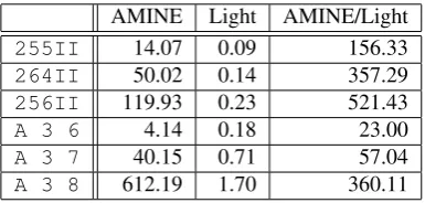
255II 14.07 0.09 156.33 264II 50.02 0.14 357.29 256II 119.93 0.23 521.43 A 3 6 4.14 0.18 23.00 A 3 7 40.15 0.71 57.04 A 3 8 612.19 1.70 360.11

Table 1: The execution times in seconds on Linux PC (2.6GHz, Pentium 4, 512MByte)

Example3 The computation ofhr |Add(r,Z) =S(Z)iis given below: ( []|[]|r| − |Add(r,Z) =S(Z) )

=⇒( []|[]|r| − |r=S(x),Z=Add(x,Z) ) (I) =⇒( [r7→S(x)]|[]|r| − |Z=Add(x,Z) ) (II.0)

=⇒( [r7→S(x)]|[]|r| − |x=Z) (I)

=⇒( [r7→S(x)][x7→Z]|[]|r| − | −) (II.0).

update( [r7→S(x)][x7→Z]|[]|r| − | −)

=update( [r7→S(Z)]|[]|r| − | −) =S(Z).

4.2 Benchmark results

We compare the lightweight version with Pinto’s implementation (AMINE). Both are written in C language. Table1shows execution times in seconds of our implementation and AMINE. The final column gives the ratio between the two. The first three input programs are applications of church numerals where n=λf.λx.fnx andI=λx.x. The encodings of these terms into interaction nets are given in [Mac98]. The next programs compute the Ackermann function. The following rules are the interaction net encoding of the Ackermann function:

Pred(Z)onZ, Dup(Z,Z)onZ,

Pred(x)_o_nS(x), Dup(S(a),S(b))_o_nS(Dup(a,b)), A(r,S(r))_o_nZ, A1(Pred(A(S(Z),r)),r)_o_nZ,

A(A1(S(x),r),r)_o_nS(x), A1(Dup(Pred(A(r1,r)),A(y,r1)),r)_o_nS(y),

andA 3 6means computation ofhr |A(S(S(S(S(S(S(Z)))))),r) =S(S(S(Z)))i.

The results that we have obtained are better than previous implementation results, and allow substantially larger classes of functions to be executed very efficiently. Depending on the archi-tecture used, these results will vary slightly. We however invite the reader to try some of these examples by downloading our implementation:http://www.interaction-nets.org/.

5 Conclusion

(13)

Implementation work for interaction nets is currently being investigated very actively, and although this step is a considerable one, we believe that there is still much more to do. Our im-plementations are still very much prototype in nature, and no program optimisations have been included here. Future work will be directed towards developing stable and efficient implementa-tions for both sequential and parallel architectures.

Bibliography

[Abr93] S. Abramsky. Computational Interpretations of Linear Logic.Theoretical Computer Science111:3–57, 1993.

[AG98] A. Asperti, S. Guerrini. The Optimal Implementation of Functional Programming Languages. Cambridge Tracts in Theoretical Computer Science 45. Cambridge Uni-versity Press, 1998.

[FM99] M. Fern´andez, I. Mackie. A Calculus for Interaction Nets. In Nadathur (ed.), Pro-ceedings of the International Conference on Principles and Practice of Declarative Programming (PPDP’99). LNCS 1702, pp. 170–187. Springer-Verlag, 1999.

ftp://lix.polytechnique.fr/pub/mackie/papers/calin.ps.gz

[GAL92] G. Gonthier, M. Abadi, J.-J. L´evy. The Geometry of Optimal Lambda Reduction. In

Proceedings of the 19th ACM Symposium on Principles of Programming Languages (POPL’92). Pp. 15–26. ACM Press, Jan. 1992.

[HMS08] A. Hassan, I. Mackie, S. Sato. Interaction nets: programming language design and implementation.ECEASST10, 2008.

[HMS09] A. Hassan, I. Mackie, S. Sato. Compilation of Interaction Nets.Electron. Notes Theor. Comput. Sci.253(4):73–90, 2009.

doi:http://dx.doi.org/10.1016/j.entcs.2009.10.018

[Laf90] Y. Lafont. Interaction Nets. InSeventeenth Annual Symposium on Principles of Pro-gramming Languages. Pp. 95–108. ACM Press, San Francisco, California, 1990.

[Mac98] I. Mackie. YALE: Yet Another Lambda Evaluator Based on Interaction Nets. In Pro-ceedings of the 3rd ACM SIGPLAN International Conference on Functional Program-ming (ICFP’98). Pp. 117–128. ACM Press, September 1998.

ftp://lix.polytechnique.fr/pub/mackie/papers/yalyal.ps.gz

[Mac05] I. Mackie. Towards a Programming Language for Interaction Nets.Electronic Notes in Theoretical Computer Science127(5):133–151, May 2005.