Copyright Undertaking

(1)

Copyright Undertaking

By reading and using the thesis, the reader understands and agrees to the following terms: 1. The reader will abide by the rules and legal ordinances governing copyright regarding the

use of the thesis.

2. The reader will use the thesis for the purpose of research or private study only and not for distribution or further reproduction or any other purpose.

3. The reader agrees to indemnify and hold the University harmless from and against any loss, damage, cost, liability or expenses arising from copyright infringement or unauthorized usage.

IMPORTANT

If you have reasons to believe that any materials in this thesis are deemed not suitable to be distributed in this form, or a copyright owner having difficulty with the material being included in our database, please contact [email protected] providing details. The Library will look into your claim and consider taking remedial action upon receipt of the written requests.

Pao Yue-kong Library, The Hong Kong Polytechnic University, Hung Hom, Kowloon, Hong Kong

(2)

EFFICIENT NUMERICAL METHODS FOR MULTI-PHASE

FLOW PROBLEMS WITH PENG-ROBINSON EQUATION OF

STATE

ZHANG YUZE

PhD

The Hong Kong Polytechnic University

(3)

(4)

The Hong Kong Polytechnic University

Department of Applied Mathematics

EFFICIENT NUMERICAL METHODS

FOR MULTI-PHASE FLOW PROBLEMS

WITH PENG-ROBINSON EQUATION

OF STATE

ZHANG YUZE

A thesis submitted in partial fulfilment of the requirements for the degree of Doctor of Philosophy

(5)

Certificate of Originality

I hereby declare that this thesis is my own work and that, to the best of my knowledge and belief, it reproduces no material previously published or written, nor material that has been accepted for the award of any other degree or diploma, except where due acknowledgement has been made in the text.

(Signature)

(6)

Abstract

This work concerns numerical simulations of diffuse interface models with Peng-Robinson equation of state (EOS). The motivation of our research arises from in-creasing attention of complex fluids flow problems in the oil industry.

There are two basic concerns in the oil industry: oil exploration and oil exploita-tion. In oil exploration, properties of petroleum substances at the equilibrium state are mainly concerned. This requires us to construct numerical schemes that can accurately capture the interface information between hydrocarbon substances and phases. In oil exploitation, some fluids flow problems with complex boundary con-ditions need to be considered. Designed numerical schemes need to have a kinetic nature and a simple algorithm structure because of the huge amount of calculation required. In this thesis, based on these two specific needs of numerical algorithms, we introduce the energy stable scheme and Lattice Boltzmann method (LBM) to solve the equilibrium and fluids flow problems, respectively.

Firstly, a Cahn-Hilliard type equation is derived to describe the single-component two-phase equilibrium problem. A first-order scalar auxiliary variable (SAV) scheme and a second-order SAV scheme are proposed to simulate the evolution process of single-component two-phase hydrocarbon substances. Mass conservation and energy stability in discrete sense are proved for these two schemes. Moreover, this approach has been expanded to the multi-component two-phase equilibrium case in this thesis. Based on the previous work [18], we modify this Cahn-Hilliard type model by

(7)

in-troducing the mobility term. This improvement makes the multi-component model more physically compatible. A second-order SAV scheme is designed to solve the multi-component model. Numerical experiments have been carried out for both the single-component case and the multi-component case. Our numerical results match well with the laboratory data. It is worth mentioning that we have improved the calculation of interface tension and capillary pressure comparing with previous work. For multi-phase fluids flow problems, in order to verify the feasibility of the LBM for oil exploitation problems, we firstly use the single-relaxation-time LBM to solve a single-component equilibrium problem based on an Allen-Cahn type equation. Then, we design a multi-phase fluids dynamics model combined with Peng-Robinson EOS with a constant temperature under thermodynamics principles. Here, we use the multi-relaxation-time (MRT) LBM combining with Beam-Warming scheme to solve the proposed fluid model. Alterable CFL numbers can be used in the numerical simulation. High-order accurate numerical results have been obtained, which meet well with our expectations and have a great agreement with previous published results and laboratory data.

Key words: Peng-Robinson equation of state, equilibrium problems, multi-phase flow problems, scalar auxiliary variable approach, Lattice Boltzmann method.

(8)

Acknowledgements

Many people have offered me valuable help in my thesis writing. First and foremost, I want to show great respect to my supervisor, Dr. Zhonghua Qiao. He is obviously the expert in the research field and supervising of students. During the past three years, he has given me considerable help by means of discussion, suggestion and comments. His encouragement and unwavering support has sustained me through frustration and depression. Without his pushing me ahead, the completion of my PhD career would be impossible. Also, he is not only the mentor of my research career but also the mentor of my life. In daily life, he always sets a good standard for me.

I would like to express my appreciation to Prof. Shuyu Sun in the King Abdullah University of Science and Technology. He showed me this interesting research topic with strong background of applications. His rich knowledge of thermodynamics and physics has helped me a lot in my research. In addition, it is a great honor to meet and discuss with Prof. Tiezheng Qian in the Hong Kong University of Science and Technology. He selflessly provided me many valuable suggestions and guided me on my research.

I would also like to thank Dr. Xuguang Yang, who is the big brother in my daily life and solid backing in the research. He taught me on the Lattice Boltzmann method and helped me to complete my thesis without any reservation. Moreover, I want to thank Dr. Xiao Li, who helped me a lot on the programming and gave me

(9)

many pieces pf helpful advice on my research. At the same time, Mr. Tao Zhang, who is my cooperator in the King Abdullah University of Science and Technology, has also played an important role during my whole PhD career.

I want to extend my sincere thanks to my close friends in the Hong Kong Poly-technic university, Mr. Junbo Chen, Mr. Chendi Wang, Mr. Meng Xiao, Mr. Dawen Yao, Mr. Boyu Zhang and Dr. Jiongyi Zhu.

Last but not least, I am deeply indebted to all my family members, who love me and bear with me. Without their encouragement and support, it is impossible for me to reach here.

(10)

List of Figures

1.1 Infinite small splitting. . . 8

1.2 Finite amount splitting. . . 11

1.3 Flowchart of the NVT flash calculation.. . . 12

2.1 The evolution history of solutions of SAV1 from a single droplet. . . . 29

2.2 The comparison between results of the SAV1 and the convex splitting

scheme (the 1D cross section of the final state). . . 29

2.3 CPU times of SAV1 and the convex splitting scheme on different meshes. 30

2.4 The evolution history of solutions of SAV1 from four droplets. . . 31

2.5 3D simulation results of the evolution ofnC4 at 350K. . . 32

2.6 The evolution history of the total mass (mol/m3_{) (Left) and the}

evo-lution history of the total free energy (Right). . . 33

2.7 The width of the interface. . . 34

2.8 The comparison of the surface tension (N/m) obtained by the

nu-merical experiment and the data from laboratory (left); The capillary pressure (Pa) calculated from the numerical results and the

Young-Laplace method (right). . . 35

2.9 Molar density distributions of methane at different time: (a) t=0, (b)

t=500, (c) t=1500. . . 43

2.10 Molar density distributions of n-decane at different time: (a) t=0, (b)

t=500, (c) t=1500. . . 44

2.11 The mass evolution of the methane (left) and n-decane (right). . . 44

(13)

2.13 The width chosen of the interface: (a) Method 1; (b) Method 2. . . . 46

2.14 Comparison of interface tension between the laboratory data and the numerical scheme.. . . 46

3.1 Numerical results ofnC4 at different time steps: (a) t=200, (b) t=500, (c) t=1000. . . 56

3.2 Numerical results ofC3 at different time steps: (a) t=100, (b) t=500, (c) t=1500, (d) t=4000. . . 57

3.3 3D profile along Z “ L{2 after convergence (nC4 at T=350K): (a) surface tension contribution of Helmholtz free energy density; (b) cross profile of (a); (c) homogeneous contribution of chemical potential; (d) cross profile of (c); (e) thermal pressure; (f) cross profile of (e). . . 59

3.4 Energy dissipation and mass conservation of 3D numerical simulation of nC4: (a) energy dissipation, (b) total mass variation with time. . . 60

3.5 Comparison of surface tension between numerical predictions and lab-oratory data; (a) nC4, (b) C3. . . 60

3.6 Comparison with Laplace law: (a) nC4, (b) C3. . . 60

3.7 Two phase coexistence curve. . . 80

3.8 Time evolution of the molar density distribution. . . 82

3.9 Time evolution of the average kinetic energy. . . 83

3.10 Time history of the average kinetic energy with different CFL numbers. 84 3.11 Time evolution of the multiple merging droplets; (a) t “ 100, (b) t“400, (c)t“1000, (d) t“2000. . . 85

3.12 Numerical validation: (a) Comparison of surface tension, (b) valida-tion of Laplace law. . . 86

(14)

List of Tables

1.1 Initial valuespmol{m3qfor the methane (n1) and n-decane (n2) in the

gas and liquid phases . . . 13

2.1 Relative errors and temporal convergence of approximation solutions for first order and second order SAV schemes (SAV1 and SAV2) on a 1024ˆ1024 uniform mesh . . . 28

3.1 Parameters of some DnQm models. . . 53

3.2 Initial molar densities of nC4. . . 56

3.3 Initial molar densities of C3. . . 56

3.4 Eφ with different lattice spacings and different CFL numbers. . . 79

3.5 Relevant data ofnC4. . . 81

(15)

Chapter 1 Introduction

1.1 Background

Modeling and numerical simulation of the multi-phase flow is a significant issue in many scientific and engineering applications, including groundwater contamination, carbon sequestration, air pollution, petroleum exploration and recovery, chemical

and biological separation processes, etc. While simulating the multi-phase flow,

especially in the oil industry, capillary pressure caused by interface tension between various fluids is one of major proprieties. Some physical properties are influenced by the capillary pressure, such as relative permeability and residual saturations. These impact the transportation of the vapor and liquid in a porous medium and bring many multiple phases problems.

In order to understand physical phenomena involving multiple phases, such as liq-uid droplets, gas bubbles and phase change and separation, it is necessary to model and simulate the interface between phases. The truth is, properties on the interface are always accompanied with complex physical activities (sometimes, chemical re-actions involved). This makes it difficult to model the phenomena on the interface between different substances or different phases. There exist several methodologies

to describe interfaces in different scales [10, 11, 14, 21, 22, 26, 79]. At the

micro-scopic scale, Molecular Dynamics and Monte Carlo method [10, 20, 83] are main

(16)

CHAPTER 1. INTRODUCTION PhD Thesis

tools to resolve the interface. Using the randomness to solve problems is its essen-tial idea and it shows great advantages when target problems combined with many coupled degrees of freedom. Besides, at the macroscopic scale, the sharp interface

model [26, 60] is a common approach while considering large-scale problems. In this

method, the interface is treated as a zero-thickness entity and molar densities of substances undergo a jump through the interface. Inter-facial conditions including interface tensions should be given to keep the nature of interfaces in the simulation. When physical properties, such as the interface tension or the capillary pressure, become the primary concern, it is obviously that the sharp interface model is not an appropriate approach to catch the interface information. Here, we introduce a continuous model to catch these properties, which is known as the diffuse-interface

model or phase-field model [2,5,6,78]. In this theory, the interface is described as a

continuum entity to separate the two bulk single-phase fluid regions. It means that molar distributions are continuous within the interface. Compared with molecular scale methods, the diffuse interface model is more efficient and it can also provide the quantity of the interface tension. In our work, we focus on the diffuse interface model and its numerical schemes.

Diffuse interface models have been extensively studied for multi-phase flow

prob-lems in recent years [4,51,67,72]. In these works, double-well Ginzburg-Landau free

energy are usually considered. This free energy can describe some interface prop-erties qualitatively. While considering some real problems that occurred in the oil industry problems, it is impossible to use quantitatively meaningful parameters of a simple double-well potential for simulations of realistic hydrocarbon species in an oil-gas two-phase system. As a result, we need realistic equation of state (EOS) to describe hydrocarbon substances. Here, we introduce Peng-Robinson EOS [54] to do the simulation. This EOS can be applicable to calculations of all fluid properties in natural hydrocarbon gas processes, which is an important part in the pore scale

(17)

PhD Thesis CHAPTER 1. INTRODUCTION

modeling and simulations of the subsurface fluid. Because of the realistic thermo-dynamics properties involved, some physical properties should be preserved when we design numerical schemes. Usually, the mass conservation law and the energy dissipation principle are two mainly concerned nature of the process. Therefore, designing numerical schemes with physical compatibility is very important.

For the diffuse-interface model with Peng-Robinson EOS, some efforts have been made in literature. For the single-component case, in [59], Qiao and Sun investigated an Allen-Cahn type two-phase single-component model with Peng-Robinson EOS in two-dimensional space while only one-dimensional problems were considered in previous applications. A convex splitting approach was developed in this work to

solve the proposed model. After that, in [33, 34, 56], energy stable schemes were

also proposed by convex splitting method. In [55], Peng proposed a Cahn-Hilliard type two-phase model with Peng-Robinson EOS and used convex splitting scheme to solve it. Recently, based on the Allen-Cahn type two-phase single-component model, an invariant energy quadratization scheme was also developed to study the Peng-Robinson EOS problems [43]. For the multi-component case, Kou and Sun proposed a multi-component two-phase model with Peng-Robinson EOS in [31], and the modified Newton’s method with a relaxation parameter was employed to solve the model. Soon after, in [18], Fan, Kou, Qiao and Sun designed a component-wise convex splitting scheme of this multi-component model. More applications of

multi-component model can be found in [32,35].

In this research, two fundamental issues in the oil industry will be studied: oil exploration and oil exploitation. For oil exploration, which concerns about physical properties on phase interfaces, we use so-called energy stable methods to solve single-component and multi-single-component two-phase equilibrium problems. Because of the physical compatibility of these algorithms, some physical properties of the system can be preserved automatically during numerical simulations. This allows us to get

(18)

laboratory-data-comparable numerical solutions. On the other hand, if we consider the oil exploitation problem with complex geometries and boundary conditions, the Lattice Boltzmann method (which is very popular in engineering calculations) is more suitable. This approach has a great compatibility for complex fluids flow problems. In this work, we mainly study the Lattice Boltzmann method for the single-component hydrocarbon fluids flow problems.

1.2 Peng-Robinson EOS in the diffuse-interface

problem

In this section, we will give a brief introduction of Peng-Robinson EOS and its Helmholtz free energy form in the diffuse-interface problem. The basic expression of Peng-Robinson EOS can be shown as

P “ nRT

1´bn´

n2apTq

1`2bn´b2_n2, (1.1)

where n “ N

V is the molar density of the substance with N representing the total

particle number and V being the total volume. a “apTq is the pressure correction

coefficient andb“bpTqis the volume correction coefficient. They are given as follows

apTq “ m ÿ i“1 m ÿ j“1 qiqjpaiajq 1 2_p1_´k ijq, bpTq “ m ÿ i“1 yibi.

Here qi represents the mole fraction of the ith component, kij represents the binary

(19)

PhD Thesis CHAPTER 1. INTRODUCTION follows aipTq “ 0.45724 R2T_ci2 Pci p1`mip1´ c T Tci qq2, bi “0.7780 RTci Pci ,

where Tci and Pci are the properties of the ith substance representing the critical

temperature and critical pressure, respectively. mi has the form

mi “0.37464`1.54226ωi´0.26992ω2i, ωi ď0.49;

mi “0.379642`1.485030ωi´0.164423ωi2`0.01666666ω

3

i;ωi ą0.49.

Using the critical data of the substance we can calculate ωi inmi above

ωi “ 3 7p log10p_{14.695P SI}Pci q Tci Tbi ´1 q.

When we consider the real inhomogeneous fluid system, in order to describe the phenomenon around the interface, the diffuse-interface model with the gradient

contribution is taken. Here, the total energy densityfpnq takes the following form

fpnq “ fbpnq `f∇pnq,

where n “ pn1,¨ ¨ ¨, nmq, m is the amount of the substances, ni “ N_Vi is the molar

density of the ith substance with Ni representing the total particle number of the

ith substance. The Helmholtz free energy fbpnq of a homogeneous fluid with

Peng-Robinson EOS is given by

fbpnq “ fbidealpnq `f excess b pnq, f_bidealpnq “ RT m ÿ i“1 niplnni´1q, f_bexcesspnq “ ´nRTlnp1´bnq ` apTqn 2?2b lnp 1` p1´?2qbn 1` p1`?2qbnq, (1.2) — 5 —

(20)

whereR“8.31432J K´1mol´1 is the gas constant,T is the temperature,n “řm_i ni.

The inhomogeneous term of the gradient contribution f∇pnq can be modeled by a

simple relation f∇pnq “ 1 2 m ÿ i,j“1 cij∇ni¨∇nj, (1.3)

where cij is the influence parameter given as follows

cij “ p1´βijq

?

cicj. (1.4)

Here,βij P r0,1qis the binary coefficient. In this research, we setβii “0 andβij “0.5

as in [35]. ci represents the influence of the pure substance given as below, which

has the relation with the pressure correction parameter and the volume correction parameter of Peng-Robinson EOS.

ci “aib 3 2 i pm c 1,ip1´ Tci T `m c 2,iqq, mc_1,i “ 10 ´16 1.2326`1.357457ωi , mc_2,i “ 10 ´16 0.9051`1.5410ωi .

1.3 Initial values of the multi-phase system

How to set the initial value of multi-component mixture is a critical modeling issue when the real EOS is introduced (Peng-Robinson EOS is involved in this work). In practice, phase splitting problems need to be considered. The NPT calculation (tem-perature T, pressure P and composition N) and the NVT flash calculation (temper-ature T, volume V and composition N) are two common phase splitting approaches. As discussed in [57], classical coupled schemes based on NPT flash calculation suffer from some essential limitations, such as the requirement of constructing a pressure

(21)

equation as there is no intrinsic pressure equation. An alternative modeling frame-work, based on the NVT flash calculation with moles, volume and temperature as

primal state variables, has been actively studied very recently [29, 30]. Flash

cal-culations allow us to get the molar density of gas and liquid of a specific substance when the phase transition occurs. It has been shown that the NVT flash calculation

is better posed than the NPT flash calculation [29, 30]. In this section, we give a

brief introduction to the NVT flash calculation. The obtained solution can be used as the initial value of diffuse-interface problems with given substances [50].

First of all, we specify the overall composition, i.e. mole fraction of each species

in the overall fluid mixture consisting n components and possibly multiple phases

and we define zi “

Ni

N as the overall mole fraction of the i-th component in the

entire mixture. Ni is the total amount of i-th component. N “

řm

i Ni and V are

the total amount and total volume, respectively. Then we will go through two steps to get molar concentrations of substances that can guarantee the phase separation numerically and the given mixture is not thermodynamic phase-stable.

At the beginning, we need to give some notations: c “ N

V is the total molar

density of the mixture and czi “

Ni

V , i “ 1,¨ ¨ ¨ , m, is the molar concentration of

i-th component. c1 _{is the trial molar density or the total molar density of the new}

phase (which can be found in Fig. 1.1, and details will be discussed shortly). c2 _{is the}

molar density of the original phase after the phase separation (which can be found in

Fig. 1.2, and details will be discussed shortly). V1

i is the volume ofi-th component in

the new phase andV2

i is the volume of of i-th component in the original phase after

the phase separation. V1

“ř_iVi1 and V2 “

ř

iV

2

i . Ni1 is the particle number of i-th

component in the new phase and N2

i is the particle number of of i-th component in

the original phase after the phase separation. N1

“ř_iN1 i and N2 “ ř iN 2 i and we — 7 —

(22)

denote ¯yi “

N2

i

N2 , i“1,¨ ¨ ¨ , m.

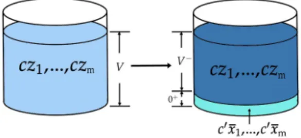
STEP 1. Infinitesimal splitting

It is believed that, if the phase splitting happens, the new phase (here we call it

the trial phase) will form with an infinitesimal volume (here we use 0` _{to describe}

this volume) at the very beginning of the phase separation. So our first step is to determine whether or not this phenomenon happens under given conditions.

Figure 1.1: Infinite small splitting.

As we can see in the Fig. 1.1, if the phenomenon happens, the original

single-phase mixture (with n components’ molar densities cz1, ..., czn) will split into the

trial phase part (infinitesimal volume part) with the volume 0` _{and the rest part}

with the volume V´

“V ´0` during the progress of the infinite small splitting. In

this step, our aim is to find the trial molar densityc1 _{of the new phase.}

First, we need to calculate the saturation pressure psat _{which has the following}

form psat “pcexpr5.37p1`ωqp1´ Tc T qs, (1.5) where ω “ 3 7p log10p_pp_atmc q Tc Tb ´1

q. Given critical properties Tc, Pc and boiling point TP of

different components, we will get different psat _{of different components. Here we}

note that patm represents the unit standard atmosphere pressure. Usually it has the

(23)

pressurepsat

i for each component, we will calculate the trial phase composition under

the framework of the NVT flash calculation.

The truth is, from the beginning, we do not know the phase state of the mixture. So we have following two assumptions.

• Case 1: If the trial phase is in the liquid phase, we first calculate the total

initial pressure by pini “ n ÿ i psat_i pTqzi, i“1,¨ ¨ ¨, m, (1.6)

and then we give the formulation of the trial phase composition (liquid-like)

¯

xi “

psat_i

pini

zi i“1,¨ ¨ ¨ , m. (1.7)

After that we calculate the compressibility factorZ of the system by solving the

following equation based on Peng-Robinson EOS (different EOS has different

formulation which respects to Z).

Z3´ p1´BqZ2 ` pA´2B´3B2qZ ´ pAB´B2´B3q “ 0, (1.8) where A“ apTcqpini R2_T2 , B “ bpini RT . (1.9)

We use all the real solutions Z of the function (1.8) to do the analysis.

• Case 2: If the trial phase is in the gas phase, first we calculate the trial phase

composition (gas-like) ¯ xi “ zi psat i Σ zj psat j i“1,¨ ¨ ¨, m. (1.10) — 9 —

(24)

Then the initial pressure are given by

pini “Σpsati pTqx¯i i“1,¨ ¨ ¨ , m. (1.11)

We can get Z in the same way as in Case 1.

We then can use the obtainedZ to calculate the total molar density of trail phase

c1 _{by the following relation (the non-ideal gas equation)}

pini “Zc1RT. (1.12)

Here, we need to mention that pini we used in (1.12) should be calculated under the

same assumption with the Z we choose.

Then we will show a method to determine whether or not the system will experi-ence a phase separation under the overall composition that we gave at the beginning. Here we introduce the tangent plane distance function D

DpT,1, c1x¯1, ..., c1x¯nq “ΣrµippT,1, c1x¯1, ..., c1x¯nqq ´µippT,1, cz1, ..., cznqqsc1x¯i´

rPppT,1, c1_x_¯

1, ..., c1x¯nqq ´PppT,1, cz1, ..., cznqqs,

(1.13)

The P here is given by (1.1). The function D is used to determine whether the

phase separation will happen. If D is less than 0, it means that there will be a

phase separation and the molar density of trial phase is c1_{. Otherwise we need to}

use anotherZ to do the same process (More details can be seen in the paper by Jiri

[50]). If we fail to find the appropriate c1 _{from all the}_Z _{we got in Case 1 and Case 2,}

we need to consider a new set ofzi for the purpose of two-phase system specification.

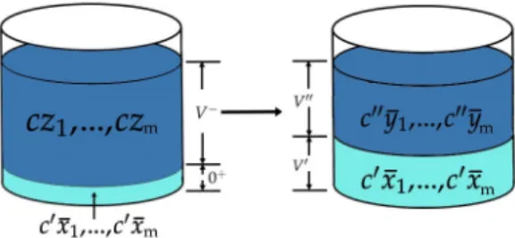
STEP 2. Finite-amount splitting

The existing of c1 _{means that the original single-phase mixture will experience the}

phase separation with the initial fraction zi. Under the assumption that the molar

(25)

composition still equals to ¯xi (which means ¯xi “

N1

i

N1) after the phase separation.

We can get molar density c2 _{, the phase composition ¯}_y

i and the total volume V2

of another phase. We call this progress the ”finite-amount splitting” and it can be

shown in the Fig. 1.2.

Figure 1.2: Finite amount splitting.

To be specific, in this step, we calculate the molar density of both phases of the i-th component by using

V1 `V2 “V, c1_V1 `c2_V2 “cV, fbpc1qV1 `fbpc2qV2´fbV ă0, (1.14)

where fb represents the Helmholtz free energy density. Here we use the bisection

method to get the values of V2 _and _c2_{. First we set} _V1 _“_0.5V _{and we can get the}

c2 _and _V2 _{by the relation}

V2 “V ´V1, c2 “ cV ´c 1_V1 V2 , (1.15)

whereV is the initial volume. For simplicity, we setV “1. Then we putc1_{, V}1_{, c}2_{, V}2

into the determination equation fbpc1qV1`fbpc2qV2´fbV ă 0. If the inequality is

established, we can get molar densities of two phases under the given thermodynamic properties.

(26)

Figure 1.3: Flowchart of the NVT flash calculation.

For multi-component systems, we can further calculate the composition of both phases by using the relation

c1_x_¯ iV1`c2y¯iV2 “cziV i“1,¨ ¨ ¨ , m, (1.16) which leads to ¯ yi “ cziV ´c1x¯iV1 c2_V2 i“1,¨ ¨ ¨ , m. (1.17)

Similarly, we can calculate ¯yi by using

fbpc1x¯1, ..., c1x¯nqV1`fbpc2y¯1, ..., c2y¯nqV2´fbpcz1, ..., cznqV ă0

as the determination function. Until now, we can get the molar concentrations c1_x_¯

i

and c2_y_¯

i of each component of different phases. We can use these molar

concen-trations as our model’s initial value npliquidq and npgasq, or we can optimize them

further using additional schemes, e.g. the method in [50].

Fig. 1.3 gives a flowchart to describe the NVT flash calculation. Based on the

above flash calculation scheme, molar density distributions of both components can be determined as the initial conditions of our further numerical simulation. For the convenience of researchers in this field, we pre-computed two-phase two-component system of the methane and the n-decane with the procedure described method. The

composition results can be found in Table1.1. In the following chapters, we will use

(27)

Table 1.1: Initial valuespmol{m3qfor the methane (n1) and n-decane (n2) in the gas

and liquid phases

Temperature (K) n1pliqq n1pgasq n2pliquidq n2pgasq

450 4062 1028 438 3522

400 3832 1428 488 2938

350 3675 1536 512 2861

300 3569 1648 564 2497

1.4 Numerical approaches

In this section, we will introduce two kinds of numerical approaches involved in this thesis. Both methods can effectively solve diffuse-interface problems, but they have different emphases.

1.4.1 Energy stable schemes for diffuse-interface models

Energy stable schemes are highly needed for large time-stepping simulations of the diffuse-interface models. Otherwise, it may require extremely small time steps to keep the energy dissipation. For a general free energy functional of the double-well potential, many energy stable schemes have been developed. To obtain an energy dissipative scheme, the linear term is usually treated implicitly in some manner, while different approaches have to be proposed for nonlinear terms. The convex splitting method is a popular method to develop energy stable schemes for diffuse-interface models. It splits the homogeneous free energy into a convex part and a concave part and treats them implicitly and explicitly in the time discretization, respectively. It was perhaps firstly studied for diffuse-interface problems in [15] but popularized by

[8, 21, 22, 72], and was proved only first-order. While it is possible to construct

second-order convex splitting schemes under certain situations (see, for instance, [63]), a general formulation of second-order convex splitting schemes is not available. Generally, nonlinear iterative solvers are needed for convex splitting schemes from a natural decomposition of energy functional. Another popular approach is the

(28)

called stabilization method, which treats the nonlinear term explicitly, and adds a stabilization term to avoid strict time step constraint. The stabilization term is usually treated implicitly and used to control the nonlinear term of the origional

model, see e.g., [3, 66] and references therein. The stabilization method generates

linear schemes and is easy to be extended to high-order schemes [28, 75], but in

general it can not be unconditionally energy stable [19, 40, 41, 42]. Recently, the

invariant energy quadratization (IEQ) approach was proposed in [9, 77] to solve a

variety of diffuse-interface models. This approach allows one to construct linear and unconditionally energy stable schemes in the sense that the modified discrete energy is non-increasing in time. However, at each time step, the linear system resulting from the IEQ approach has variable coefficients. Thus, fast calculation methods could not be used when solving the linear system because of the variable coefficient matrix. To overcome it, the so-called scalar auxiliary variable (SAV) approach was proposed

in [64, 65]. Using Cahn-Hilliard type equation as an example, it is shown that

the SAV approach has the following advantages: (i) For single-component diffuse-interface problems, it leads to, at each time step, linear equations with constant coefficients so it is remarkably easy to implement. (ii) For multi-component diffuse-interface problems, it leads to, at each time step, decoupled linear equations with constant coefficients. In our work, we will use the SAV approach to solve the diffuse-interface model with Peng-Robinson EOS for single-component and multi-component problems. For this model, many advantages could be observed in comparison to

existing energy stable schemes in [18, 43, 56, 59].

1.4.2 The Lattice Boltzmann method for multi-phase flow

problems

In the oil exploitation, many complex situations arise in porous media flow problems and pore scale simulations, such as complex geometries and boundary conditions.

(29)

Therefore, we need to develop efficient and robust methods for these problems. In recent years, the Lattice Boltzmann method (LBM), which is originated from lattice gas automata (LGA) and also could be derived from the kinetic Boltzmann equation, has emerged as an powerful method for simulating complex fluids dynamics

prob-lems [1, 7, 24]. The kinetic nature brings many advantages to the LBM, including

clear physical pictures, simple algorithm structure, easy implementation of boundary conditions and natural parallelism. In addition, it is also very easy to incorporate internal interactions between the fluid and external environment at the microscopic level, which makes the LBM very suitable for simulating component and multi-phase flows. Up to now, various types of LBMs have been constructed from different viewpoints for multi-phase and multi-component flows, such as the color-fluid model

[23], the pseudo-potential model [61, 62], the free energy model [69,70], the kinetic

model based on Enskog equation [47, 48], and the phase-field model (or

diffuse-interface model or mean-field theory model) [27, 38, 39, 80]. Among them, due to

the aforementioned attractive features, phase-field based LBM has become a widely used method for simulating multi-phase flows with low and large density ratios. The initial phase-field based LBM was proposed by He et al. [27]. In their work, two distribution functions were introduced. One is a pressure distribution function and the other one is an order parameter distribution function to track interfaces between different fluids. Whereafter, based on the work of He et al. [27], a three-stage stable scheme was developed by Lee and Lin [38]. Through discretizing gradient terms in different manners before and after the streaming step, the multi-phase flow with a large density ratio can be simulated. Later, Zheng et al. [80] proposed a modified LBM that can accurately recover the interface capturing equation, i.e. Cahn-Hilliard equation. Several improved Lattice Boltzmann models for the

Navier-Stokes-Cahn-Hilliard coupled system have been developed [44, 73, 74, 76, 82, 81]. These three

marvelous multi-phase LBMs have achieved remarkable success in simulating various — 15 —

(30)

(31)

Chapter 2 Energy stable schemes for the

equilibrium problem of

hydrocarbon substances

In this chapter, the aim of our research is to use the SAV approach to solve multi-phase problems under equilibrium conditions. These problems are mostly used to acquire some physical quantities on the interface between different phases or different substances, such as the interface tension and the capillary pressure. In this chapter, we consider the Cahn-Hilliard type equation not the Allen-Cahn type equation which is more suitable for multi-phase systems in multi-component condition. The structure of this chapter is shown as below.

First, we develop two SAV schemes to solve the single-component phase equi-librium problem in three dimensional space. After that, based on thermodynamic principles, by involving the mobility term, we give a new Cahn-Hilliard type model to describe the multi-component two-phase equilibrium problem. Then, an SAV solver is proposed to solve the developed model. All numerical results of the developed scheme will be compared with the laboratory data.

(32)

CHAPTER 2. ENERGY STABLE SCHEMES FOR THE EQUILIBRIUM

PROBLEM OF HYDROCARBON SUBSTANCES PhD Thesis

2.1 A single-component two-phase model

In order to study behaviours of oil substances in the equilibrium state, first, we need to find an appropriate way to describe the single-component equilibrium be-haviour. In this section, we will study the energy stable scheme of a single-component two-phase model and we just consider about the one component case. The multi-component problem will be discussed in the next section.

In [59], an Allen-Cahn type model was considered

$ ’ ’ ’ & ’ ’ ’ % Bn Bt ´c∆n “µ´µb, ż Ω ndx“N, (2.1) where µb “ Bfb

Bn is the chemical potential, c is the influence parameter calculated

by (1.4) while i “j and βij “ 0. µis a Lagrange multiplier to guarantee the mass

conservation of the system. It is anL2_{-gradient flow of}

F “ ż Ω fb` c 2|∇n| 2_dΩ. _(2.2)

In our work, a Cahn-Hilliard type model is considered as follows

nt`c∆2n “∆µb, (2.3)

which could preserve the mass conservation in a natural way.

(33)

PhD Thesis

CHAPTER 2. ENERGY STABLE SCHEMES FOR THE EQUILIBRIUM PROBLEM OF HYDROCARBON SUBSTANCES

2.1.1 The SAV approach for a diffuse interface model with

Peng-Robinson EOS

A. Model reformulation

Considering Eq. (2.3), we use the SAV approach to reformulate it. The homogeneous term of the free energy has the form

Ep “

ż

Ω

fbdΩ. (2.4)

We introduce the following term

rptq “aEp`C0, (2.5)

where C0 is a constant such that Ep`C0 ě0. Therefore, the total Helmholtz free

energy (2.2) can be rewritten into the form ˆ F “ ż Ω c 2|∇n| 2_dΩ `r2´C0. (2.6)

By using (2.5), the original problem can be transformed into the following system

$ ’ ’ ’ ’ ’ ’ ’ & ’ ’ ’ ’ ’ ’ ’ % nt “∆µ; µ“ ´c∇2n`a r Ep`C0 µbpnq; rt“ 1 2aEp`C0 ż Ω µbpnqntdΩ, (2.7)

which can be further simplified into

$ ’ ’ ’ & ’ ’ ’ % nt`c∆2n´ r a Ep`C0 ∆µbpnq “0, rt “ 1 2aEp`C0 ż Ω µbpnqntdΩ. (2.8)

This system has the following energy dissipation property, which could be proved in a similar way as in [59].

(34)

Lemma 2.1. The total Helmholtz free energy Fˆ satisfies the following energy law:

dFˆ

dt “ ´

ż

Ω

∇µb∇µbdx. (2.9)

Remark 2.2. (2.8) also satisfies the mass conservation d

dt

ż

Ω

ndΩ “ 0 as in [56], so it is no need to add a Lagrange multiplier as for the second order model in [59].

B. Spectral discretization

In this part, we will give notations of some spatial operators for the spectral

collo-cation method on the three-dimensional space Ω“ p0, Xq ˆ p0, Yq ˆ p0, Zq.

Let Nx, Ny, Nz be any positive even numbers, the NxˆNy ˆNk mesh Ωh of Ω

can be described as the following nodes setpxi, yj, zkq, where xi “ihx,yj “jhy and

zk “khz, 1ďi ďNx, 1ďj ďNy, 1ďk ďNz. hx “ _NX_x, hy “ _NY_y and hz “ _NZ_z. We

define index sets

Jh “ tpi, j, kq PN3|1ďiďNx,1ďj ďNy,1ďkďNzu, ˆ Jh “ tpl, m, nq PZ3| ´ Nx 2 `1ďl ď Nx 2 ,´ Ny 2 `1ďmď Ny 2 ,´ Nz 2 `1ďn ď Nz 2 u.

Then we define all the periodic grid functions on Ωh asFh, which has the following

form

Fh “ tf : Ωh ÑR|fi`lNx,j`mNy,k`nNz “fi,j,k, for anypi, j, kq PJh andpl, m, nq PZ

3

u. (2.10)

For any function f P Fh, we can define the following 3-D Fourier transform

ˆ

f “P f and the inverse Fourier transform f “P´1fˆby

ˆ fl,m,n“ 1 NxNyNz ÿ pi,j,kqPJh fi,j,kexppí 2lπ X xiqexppí 2mπ Y yjqexppí 2nπ Z zkq, pl, m, nq P ˆ Jh; fi,j,k “ ÿ ˆ fl,m,nexppi 2lπ X xiqexppi 2mπ Y yjqexppi 2nπ Z zkq, pi, j, kq PJh.

(35)

PhD Thesis

Let ˆFh “ tP f|f P Fhu. First order partial operators ˆDx , ˆDy and ˆDz are defined on

ˆ Fh as follows: pDˆxfˆql,m,n “ p 2lπi X q ˆ fl,m,n, pDˆyfˆql,m,n “ p 2mπi Y q ˆ fl,m,n, pDˆzfˆql,m,n “ p 2nπi Z q ˆ fl,m,n,

where pl, m, nq P Jˆh. Then the spectral form of second order partial operators can

be written as

D2_x “P´1Dˆ2_xP, D2_y “P´1Dˆ_y2P, D_z2 “P´1Dˆ2_zP.

Spontaneously, we can define the discrete Laplace operator ∆h as

∆hf “Dx2f `Dy2f`D2zf.

The inner product can also be denoted as

pf, gqh “h3xh 3 yh 3 z Nx ÿ i“1 Ny ÿ j“1 Nz ÿ k“1 fi,j,k¨gi,j,k.

2.1.2 A First order SAV scheme (SAV1)

In this section, we propose and analyze a first order SAV scheme. First, we assume

that the whole system is solved in the time interval r0, Ts and the space domain

Ω “ r0, Xs3. For a given positive integer Nt, we set the time step ∆t as ∆t “

T

Nt

.

For a given positive integer N, we set the grid sizeh ash“ X

N. The first order SAV

scheme is constructed by using the spectral collocation method in space as follows:

(36)

for 0ďsďNt´1, find ns`1 PFh such that

ns`1 ´ns ∆t `c∆ 2 hn s`1 ´ r s`1 a Eppnsq `C0 ∆hµbpnsq “0, (2.11) rs`1´rs “ 1 2aEppnsq `C0 pµbpnsq, ns`1´nsqh. (2.12)

Solving ns`1 _{from (2.11) leads to}

ns`1 “ p1`∆tc∆2_hq´1ns`∆t r

s`1

a

Eppnsq `C0

p1`∆tc∆2_hq´1∆hµbpnsq. (2.13)

Substituting (2.13) into (2.12) we can get the expression of rs`1 _as

rs`1 “ rs_` 1 2aEppnsq `C0 pµbpnsq,rp1`∆tc∆2hq ´1 ´1snsqh 1´ ∆t 2pEppnsq `C0q pµbpnsq,p1`∆tc∆2hq ´1 ∆hµbpnsqqh . (2.14)

In order to get ns`1_{, we need to solve (2.14) to get} _rs`1 _{firstly. Then we substitute}

rs`1 _{into (2.13) and get} _ns`1_.

Theorem 2.1. The first order SAV scheme (2.11)-(2.12) is unconditionally energy

stable, meaning that for any time step size ∆tą0,

ˆ

Fs`1´Fˆs ď0. (2.15)

Proof. First, we consider the discrete form of (2.7)

$ ’ ’ ’ ’ ’ ’ ’ ’ ’ ’ & ’ ’ ’ ’ ’ ’ ’ ’ ’ ’ % ns`1ńs ∆t “∆hµ s`1_; µk`1 “ ć∆hns`1` rs`1 a Es p `C0 µs_b; rs`1 ´rs ∆t “ 1 2aEs_`_C pµ s b, ns`1ńs ∆t qh. (2.16)

(37)

PhD Thesis

Then we take the discrete inner product of the first two functions of (2.16) withµs`1_,

ns`1_´_ns

∆t respectively and multiply the last function of (2.16) with 2r

s`1_.

Then we can get

$ ’ ’ ’ ’ ’ ’ ’ ’ ’ ’ ’ ’ & ’ ’ ’ ’ ’ ’ ’ ’ ’ ’ ’ ’ % pµs`1,n s`1 ńs ∆t qh “ p∆hµ s`1_{, µ}s`1 qh; pµs`1,n s`1 _´_ns ∆t qh “ pć∆n s`1_,ns`1 ńs dt qh` rs`1 b Ek p `C0 pµk_b,n s`1_´_ns ∆t q; 2rs`1r s`1 ´rs ∆t “ rs`1 b Ek p `C0 pµk_b,n s`1 ńs ∆t qh. (2.17) According to (2.17), we can get

p∆hµs`1, µs`1qh “ pć∆hns`1, ns`1 ńs ∆t qh`2r s`1rs`1´rs ∆t “ 1 2∆trpć∆hn s`1_{, n}s`1 qh´ pć∆hns, nsqh` pć∆hpns`1ńsq, ns`1ńsqhs ` 1 ∆tppr s`1 q2´ prsq2 ` prs`1´rsq2q “ 1 ∆tp ˆ Fk`1´Fˆkq ` 1 2∆trpć∆hpn s`1 ńsq, ns`1ńsqh`2prs`1 ´rsq2s. (2.18)

Note that ∆h is a non-positive symmetric operator. So from (2.18), we conclude that

ˆ

Fs`1´Fˆs ď0.

Theorem 2.2. The first order SAV scheme (2.11)-(2.12) can preserve the total mass

of the system as follows

N ÿ i“1 N ÿ j“1 N ÿ k“1 ns`1_i,j,kh3 “ N ÿ i“1 N ÿ j“1 N ÿ k“1 ns_i,j,kh3. (2.19) — 23 —

(38)

Proof. From (2.11), we can get N ÿ i“1 N ÿ j“1 N ÿ k“1 ns`1_i,j,k´ns i,j,k ∆t h 3 “ N ÿ i“1 N ÿ j“1 N ÿ k“1 r´c∆2hn s`1 i,j,k` rs`1 a Eppnsq `C0 ∆hµbpnsi,j,kqsh 3_. (2.20) Under the periodic boundary condition, we can find that the right hand side of (2.20) equals to zero. Thus we have

N ÿ i“1 N ÿ j“1 N ÿ k“1 ns`1_i,j,kh3 “ N ÿ i“1 N ÿ j“1 N ÿ k“1 ns_i,j,kh3. (2.21)

2.1.3 A Second order SAV scheme (SAV2)

In this section, based on the Crank-Nicolson (CN) method, we construct a second-order SAV scheme as follows

For 0 ďsďNt´1, find ns`1 PFh such that

ns`1´ns ∆t ` c 2∆ 2 hpn s`1 `nsq ´ r s`1 `rs 2 b Eppnˆs` 1 2_{q `}C₀ ∆hµbpnˆs` 1 2_{q “}0, (2.22) rs`1´rs “ 1 2 b Eppnˆs` 1 2_{q `}C₀ pµbpnˆs` 1 2_q,_pns`1_´ns_qq_h, (2.23)

where ˆns`12 can be regraded as an explicit approximation of ns`

1

2. However, due to

the highly nonlinearity of the Helmholtz free energy from Peng-Robinson EOS, it

has a strictly constraint on the time step ∆t using the explicit approximation. So

we employ the following equation for solving ˆns`12

ˆ ns`12 _´ns ∆t{2 “ ´c∆ 2 hnˆ s`1 2 _`∆ hµbpnsq. (2.24)

(39)

PhD Thesis

Then solving ns`1 _{from (2.22) leads to}

ns`1 “ p1`1 2∆tc∆ 2 hq ´1 p1´1 2∆tc∆ 2 hqn s `∆t r s`1 `rs 2 b Eppnˆs` 1 2_{q `}C₀ p1`∆tc∆2_hq´1∆hµbpnˆs` 1 2_q. (2.25) Substituting (2.25) into (2.23), rs`1 “rrs` p µbpn s`1₂ q 2 b Eppˆns` 1 2_{q `}C₀ ,rp1`∆t1 2c∆ 2 hq ´1 p1´∆t1 2c∆ 2 hq ´1sn s ∆tqh ` p∆t r s_µ bpˆns` 1 2_q 4Eppnˆs` 1 2_{q `}C₀ ,p1`∆t1 2c∆ 2 hq ´1_∆ hµbpnˆs` 1 2_qq_h_s{ r1´ p∆t µbpnˆ s`1₂ q 4Eppnˆs` 1 2_{q `}C₀ ,p1`∆t1 2c∆ 2 hq ´1 ∆hµbpnˆs` 1 2_qq_h_s. (2.26)

In order to get ns`1_{, first, we need to solve (2.26) to get} _rs`1_{. Then we substitute}

rs`1 _{into (2.25) and get} _ns`1_.

Theorem 2.3. The second order SAV scheme (2.22)-(2.23) is unconditionally energy

stable, meaning that for any time step size ∆tą0,

ˆ

Fs`1´Fˆs ď0. (2.27)

Proof. First, we consider the discrete form of (2.7)

$ ’ ’ ’ ’ ’ ’ ’ ’ ’ ’ ’ ’ & ’ ’ ’ ’ ’ ’ ’ ’ ’ ’ ’ ’ % ns`1_´_ns ∆t “∆hµ s`1₂_; µs`12 _{“ ´}C 2∆hpn s`1 `nsq ` r s`1_`_rs 2 b Eppnˆs` 1 2_{q `}C₀ µbpnˆs` 1 2_q; rs`1´rs ∆t “ 1 2 b Eppˆns` 1 2_{q `}C₀ pµbpnˆs` 1 2_q,n s`1 ´ns ∆t qh. (2.28)

Then we take the discrete inner product on the first two equations of (2.28) with

µs`1₂ _and n

s`1_´_ns

∆t respectively and multiply r

s`1_`_rs _{with the last equation. We}

(40)

can get $ ’ ’ ’ ’ ’ ’ ’ ’ ’ ’ ’ ’ ’ ’ ’ ’ ’ & ’ ’ ’ ’ ’ ’ ’ ’ ’ ’ ’ ’ ’ ’ ’ ’ ’ % pn s`1 ńs ∆t , µ s`1₂ qh “ p∆hµs` 1 2, µs` 1 2_q h, pn s`1 ńs ∆t , µ s`1₂ qh “ p´ c 2∆hpn s`1 `nsq,n s`1 ńs ∆t qh ` r s`1_`_rs 2 b Eppnˆs` 1 2_{q `}C₀ pµbpˆns` 1 2_q,n s`1_´_ns ∆t qh, prs`1q2´ prsq2 ∆t “ rs`1`rs 2 b Eppnˆs` 1 2_{q `}C₀ pµbpˆns` 1 2_q,n s`1 ńs ∆t qh. (2.29)

According to (2.29), we can get

p∆hµs` 1 2, µs` 1 2_q_h _{“ p´}c 2∆hpn s`1 `nsq,n s`1 ´ns ∆t qh` prs`1q2´ prsq2 ∆t “ 1 ∆tp ˆ Fs`1´Fˆsq. (2.30)

Note that ∆h is a non-positive symmetric operator, so we have

ˆ

Fs`1´Fˆs ď0.

Theorem 2.4. The second-order SAV scheme (2.22)-(2.23) can preserve the total

mass of the system as follows

N ÿ i“1 N ÿ j“1 N ÿ k“1 ns`1_i,j,kh3 “ N ÿ i“1 N ÿ j“1 N ÿ k“1 ns_i,j,kh3. (2.31)

The proof of mass conservation is similar as that of the first-order SAV scheme. Here we do not show details of the proof.

Remark 2.3. For both first order and second order SAV schemes (2.11)-(2.12) and

(41)

PhD Thesis

time step. This is very different from the IEQ scheme, which has the variable coeffi-cient. Constant coefficient makes it possible to use the fast Fourier transformation to solve the linear system. This will greatly reduce the computational cost in numerical simulations.

2.1.4 Numerical experiments

A. Convergence test

Numerical experiments are designed in two dimensional space to demonstrate the

temporal accuracy of presented SAV schemes. For the initial configuration, we

adopt the case of single droplet. The liquid density of isobutane under a

satu-rated pressure condition at the temperature 350K is imposed in the square subre-gion, and a saturated gas of isobutene under the same temperature is full of the rest of the domain. In this part, in order to test the convergence of the schemes, we choose a smooth initial value. The refinement test is performed with time steps

∆t “ 2ˆ10´4,1ˆ10´4,5 ˆ10´5,2.5ˆ10´5,1.25ˆ10´5 for both first and

sec-ond order schemes, and the solution obtained by secsec-ond order SAV schemes with

∆t “ 1.25ˆ10´6 is selected as the benchmark solution for computing errors. The

space is discretized by using the spectral method on the uniform 1024ˆ1024 mesh

of the domain Ω to remove the effect of errors from spatial discretization. We define the relative error by

Error“ ||n˚´nh||

||n˚||

, (2.32)

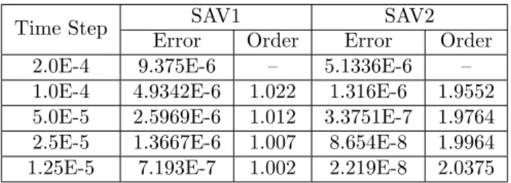
where n˚ is the benchmark solution and nh is the numerical solution on Ωh. Table

2.1 lists relative errors and convergence rates of numerical solutions att“0.05 with

different time step sizes. It is obvious that both first and second order schemes show expected accuracies. In addition, the second order scheme gives much better accuracy than the first order one.

(42)

Table 2.1: Relative errors and temporal convergence of approximation solutions for

first order and second order SAV schemes (SAV1 and SAV2) on a 1024ˆ1024 uniform

mesh

Time Step SAV1 SAV2

Error Order Error Order

2.0E-4 9.375E-6 – 5.1336E-6 –

1.0E-4 4.9342E-6 1.022 1.316E-6 1.9552

5.0E-5 2.5969E-6 1.012 3.3751E-7 1.9764

2.5E-5 1.3667E-6 1.007 8.654E-8 1.9964

1.25E-5 7.193E-7 1.002 2.219E-8 2.0375

B. Scheme verification

In this section, we simulate the separation of two phases of isobutane (nC4) at the temperature around 250K to 350K. First order SAV scheme (SAV1) and first-order

convex splitting scheme will be compared in this experiment. The computation

domain is a two-dimensional area Ω“ p0ˆLDq2, andLD “2ˆ10´8 meters. In the

two-dimensional simulation, the discrete domain has 200ˆ200 uniformed rectangular

meshes. The time step is 10´4_.

Firstly, Fig. 2.1shows the evolution of the solution of SAV1. The initial condition

is to impose the liquid nC4 under the saturated steam pressure at 350K in the region

ofp0.3LD,0.7LDq2. The rest of the domain is filled with the gas nC4 under the same

external condition. It is obviously that the gas-liquid interface formed within the whole process and the shape of the liquid drop becomes circle finally. This process meets well with the classical convex splitting scheme in the literature, as in [17] and [56].

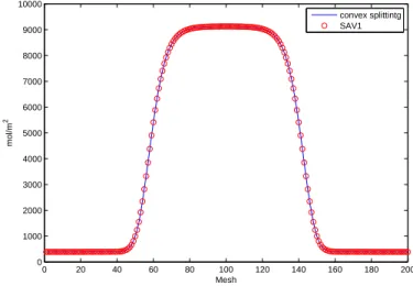
With the same initial value and boundary condition, it can be referred from Fig.

2.2that when the system reach to the stable state, both schemes give similar results.

The two curves meet very well. However, the calculation time of the SAV scheme is

much smaller than that of the convex splitting scheme. Fig. 2.3 shows CPU times of

(43)

PhD Thesis

CHAPTER 2. ENERGY STABLE SCHEMES FOR THE EQUILIBRIUM PROBLEM OF HYDROCARBON SUBSTANCES t = 0 50 100 150 200 20 40 60 80 100 120 140 160 180 200 1000 2000 3000 4000 5000 6000 7000 8000 t = 100 50 100 150 200 20 40 60 80 100 120 140 160 180 200 1000 2000 3000 4000 5000 6000 7000 8000 9000 t = 400 50 100 150 200 20 40 60 80 100 120 140 160 180 200 1000 2000 3000 4000 5000 6000 7000 8000 9000 t = 2000 50 100 150 200 20 40 60 80 100 120 140 160 180 200 1000 2000 3000 4000 5000 6000 7000 8000 9000

Figure 2.1: The evolution history of solutions of SAV1 from a single droplet.

the convex splitting scheme in this simulation.

0 20 40 60 80 100 120 140 160 180 200 0 1000 2000 3000 4000 5000 6000 7000 8000 9000 10000 Mesh mol/m 2 convex splittintg SAV1

Figure 2.2: The comparison between results of the SAV1 and the convex splitting scheme (the 1D cross section of the final state).

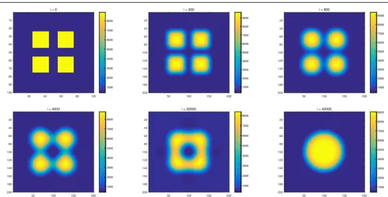
Then, we compute another benchmark problem to test the feasibility of algorithm. In this problem, the computation area is still Ω and this time we put four square

(44)

0 200 400 600 800 1000 mesh size 0 100 200 300 400 500 600 CPU time(s) SAV1 convex-spliting

Figure 2.3: CPU times of SAV1 and the convex splitting scheme on different meshes.

liquid drops in the middle of the gas region. Theoretically, firstly, the four drops start to go through the same progress as the single drop case. Then, when their shapes become round, the interface of the drops will contact with each other. Under the force of the surface tension, physically, these four liquid drops will become one big

drop. As we can see in the Fig. 2.4, our numerical results can perfectly reproduce

(45)

PhD Thesis

i = 0 20 40 60 80 100 10 20 30 40 50 60 70 80 90 100 1000 2000 3000 4000 5000 6000 7000 8000 i = 200 50 100 150 200 20 40 60 80 100 120 140 160 180 200 1000 2000 3000 4000 5000 6000 7000 8000 9000 i = 800 50 100 150 200 20 40 60 80 100 120 140 160 180 200 1000 2000 3000 4000 5000 6000 7000 8000 9000 i = 4000 50 100 150 200 20 40 60 80 100 120 140 160 180 200 1000 2000 3000 4000 5000 6000 7000 8000 i = 20000 50 100 150 200 20 40 60 80 100 120 140 160 180 200 1000 2000 3000 4000 5000 6000 7000 8000 i = 40000 50 100 150 200 20 40 60 80 100 120 140 160 180 200 1000 2000 3000 4000 5000 6000 7000 8000 9000

Figure 2.4: The evolution history of solutions of SAV1 from four droplets.

C. 3D simulation

The efficiency and accuracy of presented SAV schemes have been verified. Now we use the second order SAV scheme (2.22)-(2.22) for three dimensional simulations

to compare with laboratory data. The whole domain can be represented by Ω “

p0ˆLDq3. A uniform mesh is of 200ˆ200ˆ200 grids and the time step is taken

as ∆t “ 0.0001. In the initial condition, the liquid phase of nC4 is imposed at

350K in the region of p0.3L,0.7Lq3, and the rest domain is full ofnC4 in gas phase.

Here initial values of the liquid molar density and gas molar density are 8878.893849

mol{m3 and 403.172584 mol{m3, respectively. Fig. 2.5 shows the evolution history

of the solution which describes a cube liquid droplet turning its shape into a perfect ball shape by the force of the surface tension. The 3D simulation only takes a few minutes to reach the final state.

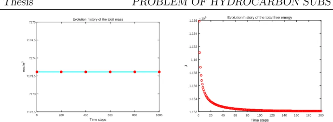
Fig. 2.6 shows the evolution history of the total energy and total mass of the

system that solved by SAV2. An obvious dissipative trend has been observed during the evolution history of the total Helmholtz free energy, with a sharp decline at the start and gradually flat in the later time. In the mean time, the mass conservation

(46)

t= 1 50 200 100 200 150 150 150 200 100 100 50 50 50 200 100 200 150 150 t= 1000 150 200 100 100 50 50 50 200 100 200 150 150 t= 3000 150 200 100 100 50 50

Figure 2.5: 3D simulation results of the evolution of nC4 at 350K.

property has also been maintained during the whole process. Here, the mass is represented by molar density. Assuming that the volume of the droplet does not change with time and that the steady state droplet has a perfect circular shape, we

make the comparison between the surface tension (N{m) obtained by the numerical

experiment and the data from laboratory. Also, we make the comparison between the capillary pressure (P a) calculated from numerical results and the Young-Laplace method. The surface tension is the net contractive force per unit length of the

(47)

PhD Thesis

0 200 400 600 800 1000 Time steps 7172.5 7173 7173.5 7174 7174.5 7175 mol/m 3

Evolution history of the total mass

0 20 40 60 80 100 120 140 160 180 200 Time steps 1.152 1.154 1.156 1.158 1.16 1.162 1.164 1.166 J

×108 Evolution history of the total free energy

Figure 2.6: The evolution history of the total mass (mol/m3_{) (Left) and the evolution}

history of the total free energy (Right).

interface which has the following form

σsur “

Fpnq ´Fpninitialq

A , (2.33)

where A is the cross surface area of the liquid droplet. In our 3D simulation, the

volume of the liquid droplet is

Vd “

4

3πr

3

“ p0.4ˆLDq3. (2.34)

After evaluating r from (2.34), we could get A “ 4πr2. In the previous work, Qiao

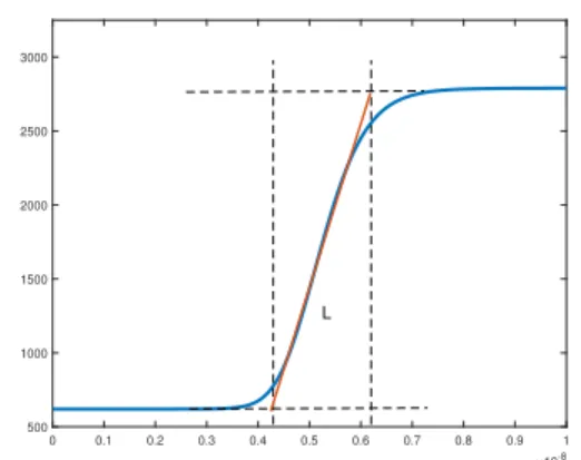
and Sun [59] set the radius of the liquid drop under the assumption that the volume of the drop does not change all along the experiment. This assumption comes from the sharp interface theory. In the same way, Li et al. [43] used the same method to calculate the surface tension. On the other hand, our numerical experiment is based on the diffuse interface theory. When we calculate the cross surface area of the droplet, the thickness of the interface needs to be considered. The determination of

the width of the interfaceLis illustrated in Fig. 2.7. So we could get the cross surface

area of the droplet as A “4πpr` L₂q2. We can see from the left figure in (2.8), the

difference between the surface tension trend calculated by the steady state of (2.23) and the experimental data, which comes mainly from modeling errors, is much better than that in paper [43] due to the improvement on surface width treatment. That

(48)

0 0.1 0.2 0.3 0.4 0.5 0.6 0.7 0.8 0.9 1 10-8 500 1000 1500 2000 2500 3000 L

Figure 2.7: The width of the interface.

makes our result more acceptable from the engineering point of view. Therefore, we could calculate another physical quality, capillary pressure, which is also of major concerns in two phase flow problems, based on the value of surface tension provided

by the fourth-order parabolic equation. The relation between the surface tension σ

and the capillary pressure,PC, could be represented by the Young-Laplace equation

in the form as

PC “Pliquid´Pgas “

2σ

r . (2.35)

Here the thermodynamic pressure for the liquid Pliquid or the gas Pgas is defined by

(1.1). Based on this formula, we could obtain the capillary pressure by applying the previously calculated value of the surface tension divided by radius, and depicted by

the right figure in Fig. 2.8. It could be observed that, the capillary pressure obtained

from our method and the previous literature are in nice agreement, which guarantees the reliability of the model (2.3) and our proposed numerical schemes.

2.2 A multi-component two-phase flow model

It is well known that, in the oil exploration and oil gathering problem, the multi-component and multi-phase problem is an unavoidable problem. For this kind of multi-component problem along with Peng-Robinson EOS, Fan etc. [18] proposed a

(49)

PhD Thesis

255 270 285 300 315 330 Temperature (K) 0.006 0.008 0.01 0.012 0.014 0.016 0.018 Interface Tension (N/m) SAV2 Laboratory data Result by Qiao and Sun [22]

255 270 285 300 315 330 350 Temperature (K) 1 1.5 2 2.5 3 3.5

Capillary Pressure (Pa)

×106

Results from Young Laplace SAV2

Figure 2.8: The comparison of the surface tension (N/m) obtained by the numer-ical experiment and the data from laboratory (left); The capillary pressure (Pa) calculated from the numerical results and the Young-Laplace method (right).

component-wise convex splitting scheme. However, during the numerical experiment, we found the model in their multi-component model is very sensible with very strict space time grid. As a result, we modify their model by involving the mobility term. After that, we use the SAV approach to solve the multi-component multi-phase system.

2.2.1 A diffuse-interface model of multi-component flows

While modeling the multi-component system, the mobility tensor is a significant element to be considered. Mobility, which is a variable defined in phase field models, plays an essential role to keep the developed model consistent with thermodynamic

laws. The mobility matrix M shall be symmetric and positive semi-definite so that

Onsager’s reciprocal principle and the second law of thermodynamics are satisfied. Different methods have been proposed to model the mobility tensor, which could be summarized into three types. The first one is to define mobility as a diagonal matrix with positive diagonal elements, which satisfies the above two principles, and is convenient to implement. Only the diffusivity of each component is considered,

so that the mobility tensor could be represented simply as: Mii. The second one is

to take mobility matrix as a full matrix, and we have two tensors Mii and Mij. It

(50)

should be noted that the mole mean diffusivity matrixDhas properties with matrix

elementsDii“0 andDij ą0. The third one is to use mass mean diffusivity instead

of mole mean diffusivity. In this section, inspiring from the first choice of mobility, we propose a new multi-component two-phase diffuse-interface model in order to use certain fast calculation approaches.

We now formulate a thermodynamic consistent mathematical model to describe the multi-component two-phase flow based on Peng-Robinson EOS, which is widely used in practice especially in petroleum industry, as it can accurately represent the thermodynamic properties of hydrocarbon mixture in the multi-phase fluids flow with the capability of handling large set of components and a large range of environment conditions. As a start, we model the flow under an isothermal condition, i.e. with a constant temperature.

The general framework we choose here is still Cahn-Hilliard type model. This is because when we consider the multi-component problem, Allen-Cahn type model can not describe the multi-component mixture. The multi-component Cahn-Hilliard model with Peng-Robinson equation of state can be written as the following form

Bni Bt `∇¨Ji “0, Ji “ ´ m ÿ j“1 Mij∇µj, (2.36)

for i “ 1,2, ..., m. Here ni, Ji and µi are the molar density, the diffusive flux and

the total chemical potential of the i-th component, respectively. M “ pMijqmˆm is

the mobility tensor, which should be symmetric and at least positive semi-definite (and in most cases, strictly positive definite) to satisfy Onsager’s reciprocal principle and the second law of thermodynamics. In [35], Kou and Sun introduced several approaches to form the mobility term. In our work, we give a new approach of

(51)

PhD Thesis

M by using a diagonal matrix with positive diagonal elements to meet the above

requirements. We set Mii“ Di N0 i |Ω| RT , i“1,2,¨ ¨ ¨ , m, (2.37) where N0

i is the total particle amount of the i-th component at the initial state and

|Ω| is the calculated volume (area in 2D). R stands for the universal gas constant

and Di ą0 is the diffusion coefficient of component i. Therefore, the diffusion flux

can be written as Ji “ ´ Di N_i0 |Ω| RT ∇µi, i“1,2,¨ ¨ ¨, m. (2.38) We need to mention that the above modeling of mobility by a diagonal matrix allows us to design certain fast calculation numerical schemes (such the SAV scheme studied in this thesis) because of its constant coefficients.

Using the mobility (2.38), the origin problem can be rewritten as

Bni

Bt `∇¨Ji “0,

Ji “ ´Mii∇µi,

(2.39)

fori“1,2,¨ ¨ ¨ , m. The total chemical potential of thei-th componentµi as used in

(2.36) has the bulk contribution µb,i and the gradient contribution µ∆,i:

µi “µb,i´µ∆,i “µb,i´

m

ÿ

j“1

cij∆nj, (2.40)

where the influence parameter cij is usually assumed to be a constant and its

ex-pression we have already given in (1.4). The bulk part µb,i is the derivative of the

bulk Helmholtz free energy density fb with respect to ni. The expression of fb in

Peng-Robinson EOS case can also be found in (1.2). The Helmholtz free energy of the total system are defined as

F “Fb`F∇, (2.41)

(52)

where Fb “ ż Ω fbpnqdx, F∇“ 1 2 ż Ω m ÿ i m ÿ j cij∇ni¨∇njdx. (2.42)

Next, an SAV scheme will be introduced to solve (2.39) for multi-component two-phase fluids flow problems.

2.2.2 The SAV approach of the multi-component model with

Peng-Robinson EOS

A. Model reformulation

Considering the multi-component two-phase model (2.39), we use the SAV approach

to reformulate it. First, we introduce _Vptq, which has the following form

Vptq “ d Fb` m ÿ i“1 CT ,iNit. (2.43)

Here, CT,i ě 0 is the thermodynamic coefficient of component i to ensure Fb `

řm

i“1CT ,iNit ě 0, and we need to choose the CT ,i based on the temperature T but

independent of the molar density. One thing we would like to mention here is that

Fb is always larger than 0 during all numerical experiments we carried out for real

substances. Using _Vptq to rewrite the chemical potential, we can get

µi “ V ptq a Fb` řm i“1CT ,iN t i µb,i´ m ÿ j“1 cij∆nj. (2.44)

Copyright Undertaking