AUSTRALIAN JOURNAL OF BASIC AND
APPLIED SCIENCES
ISSN:1991-8178 EISSN: 2309-8414 Journal home page: www.ajbasweb.com
Open Access Journal
Published BY AENSI Publication
© 2016 AENSI Publisher All rights reserved
This work is licensed under the Creative Commons Attribution International License (CC BY).
http://creativecommons.org/licenses/by/4.0/
To Cite This Article: Claudia Grace Rajakumari V. and Nesasudha M., Target Tracking in Wireless Sensor Networks using Kalman Algorithm. Aust. J. Basic & Appl. Sci., 10(5): 7-12, 2016
Target Tracking in Wireless Sensor Networks using Kalman Algorithm
Claudia Grace Rajakumari V. and Nesasudha M.
Karunya University, Coimbatore, India
Address For Correspondence:
Claudia Grace Rajakumari V., Karunya University, Coimbatore, India
A R T I C L E I N F O A B S T R A C T Article history:
Received 12 January 2016 Accepted 22 February 2016 Available online 1 March 2016
Keywords:
Wireless sensor networks, Target Tracking, Kalman Filter.
Target tracking is one of the most important applications of Wireless Sensor Networks (WSN). Wireless sensor nodes provide accurate information since they can be deployed and operated near the phenomenon. These nodes have the possibility of collaboration among themselves for the progress of target detection and tracking precisions. Target tracking in a Wireless Sensor Network (WSN) environment servers as a challenging research topic. There are many schemes for accurate target tracking. Those target tracking schemes used in WSN employ many methods which fails to track the target accurately due to non-availability of target data at regular intervals and missing of packets. Though existing tracking schemes in WSN scheme detects the target, it fails to identify the target. This work is done to overcome these problems, with the help of Kalman filter to handle maneuvering targets and multiple sensors to detect and identify the targets. This project proposes the design and working of a Kalman filter in order to locate and track an object. The target’s position from the network, is given as the input to the Kalman filter which works in a recursive manner to find the next position of the object. The implementation was done in MATLAB 7.10.0(R2010a) environment and simulation results are presented.
INTRODUCTION
The wireless sensor networks which is also called as wireless sensor and actor networks are spatially distributed autonomous sensors to monitor physical or environmental conditions, like temperature, pressure and so on. Then they cooperatively pass their data through the network to the main location. The WSN development is encouraged mainly by military applications such as battlefield surveillance. These are applied in industrial process monitoring and control, machine health monitoring, and so on (Dallil.A et al). One of the important application of wireless sensor network is target tracking. (Li. D, K. Wong et al)
Target Tracking:
While tracking a target two major problems are identified:
• The object can be tracked only if it does not move beyond the searched region.
• The appearance of the target can be affected by factors such as lighting and occlusions, which leads to inaccurate tracking.(Sandy Mahfouz et al)
Predicting the location of the target, and searching in a region centered around that location will solve these problems. This can be done using Kalman filter and hence it was proposed for target tracking (P.H. Tseng, K.T. Feng)
Methodology: Kalman filter:
A famous paper describing a recursive solution to the discrete-data linear filtering problem was published by, R.E. Kalman in 1960 after which the Kalman filter became a most common subject of research and application (L. Zhang et al). Kalman filter is a linear quadratic estimator which produces the estimates of the current state variables and it is the elementary filter for all the other models (S. Vasuhi et.al). As the next step the corrupted next measurement is observed and updated using a weighted average. All the variables are Gaussian distributed. Additional past information is not required since this algorithm is recursive. The Kalman filter normally operates as a predictor and a corrector. So the two steps involved are Prediction and updation. In order to project forward the current state and error covariance estimates thereby obtaining the a priori estimate for the next time step, the prediction process is carried out. The update equations are responsible for the feedback which gives an improved estimate when a new measurement is incorporated into the a priori estimate. The predictor equations initially predicts and projects the current state estimate ahead in time. The predicted measurements are updated by a weighted average which is the Kalman gain with the help of update equations. As we know that Kalman filter is recursive in nature, the entire process is repeated with the previous measurements in order to predict the new estimate. This recursive nature of Kalman filter is very helpful in tracking of the target in sensor networks.
Mathematical Modelling:
The Kalman filter initially assumes the state of a system at a time t obtained from the previous state at time t-1 according to the equation,
Where
(1)
• is the state vector containing the terms of interest for the system
• is the vector containing any control inputs .
• is the state transition matrix which applies the effect of each system state parameter at time t-1 on the system state at time t .
• is the control input matrix which applies the effect of each control input parameter in the vector on the state vector.
• is the vector containing the process noise terms for each parameter in the state vector. The process noise is assumed to be drawn from a zero mean multivariate normal distribution with covariance given by the covariance matrix .
Measurements of the system can also be performed, according to the model
Where
• is the vector of measurements
• is the transformation matrix that maps the state vector parameters into the measurement domain.
• is the vector containing the measurement noise terms for each observation in the measurement vector. Like the process noise, the measurement noise is assumed to be zero mean Gaussian white noise with covariance .
The initial state vector contains the position and velocity of the object.
= (3)
Then the force applied as and the mass of the object m is stored in the control vector
m
F
t=
t
The force applied during the time period Δt and the position of the object are related and written in matrix form as
= (5)
On comparing with (1) we get,
(6)
(7)
The Kalman filter algorithm involves two stages:
• Prediction
• Measurement update.
Prediction Stage:
The standard Kalman filter equations for the prediction stage are
(8)
= + (9)
where is the process noise covariance matrix associated with noisy control inputs.
In the prediction step the next estimate is predicted with the knowledge of the initial state Since KF is based on Gaussian distributinon, the variances and covariances of the variables are also predicted and stored in the matrix The Kalman filter is known to be the optimal estimator in case of a standardized one-dimensional linear system with measurement errors associated with a zero-mean Gaussian distribution.
Measurement Update:
The next step is to update the measurements that were predicted in the previous step. This update requires calculation of Kalman gain.
Thus the measurement update equations are given by
(10)
= - (11)
is the Kalman gain and is given by
(12)
The Gaussian pdfs of the predicted value and the measured value should be calculated in order to find the next estimate. The information about the state of the system is obtained from various sensors. Sometimes the
units and the scales may not be the same for all the variables. So the sensors are modelled with a new matrix .
Due to the uncertainty some states tend to be more likely than the other. The two Gaussian blobs are: One surrounding the mean of our transformed prediction, and one surrounding the actual sensor reading we got. Now both these pdfs are multiplied to find the maximum likelihood. Thus the pdfs tend to overlap hence resulting in the final estimate. This process is repeated to track the entire path of the object.
Mathematically,
PDF of the predicted state is given as
/2 (13)
PDF of the Observed or measured state is given as
/2 (14)
On multiplying both we get the final estimate as,
/2 (15)
Where
• = . + / ( + )
• = +( ( - ))/ ( + )
• = . – [ / ( + )]
RESULTS AND DISCUSSION
The simulation tool used here is Matlab 7.10.0(2010a). With assumed values of the position and velocity the input to the kalman filter that is the initial path of the object corresponding to equation (1) is generated. The graph obtained is shown in figure 1.
Fig. 1: Initial state.
With assumed values of the position and velocity the path of the object according to the observer or the measured state of the object corresponding to equation (2) is generated.
Fig. 2: Observed or Measured state.
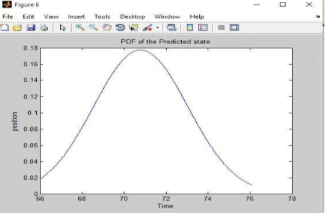
With these inputs the kalman filtering is carried on as per the mathematic modelling. These inputs undergo two stages Prediction and Updation and then the final estimate is determined. According to the Mathematical modelling multiplication of the two Gaussian PDF’s should be done. Firstly, the PDF of the Predicted state is determined and the graph figure 3 is obtained.
Fig. 3: PDF of the Predicted state.
Fig. 4: PDF of the Observed value.
On multiplying the predicted path and the path the final estimate obtained and the graph is obtained as shown in the figure 5
Fig. 5: PDF of the Final Estimate which is obtained on multiplying the PDF of Predicted state and the.
PDF of Observed state:
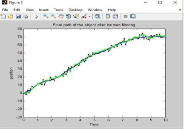
Finally, as these values are equated to the update equations, we get the path of the object that we are tracking. As the initial state and filtered output are plotted together the graph obtained is shown in the figure 6. From this graph the Initial Path and the path after filtering is found to be more or less the same since the error has been removed during the filtering process.
Fig. 6: Predicted Path of the object after Kalman filtering.
Conclusion:
object under considerstion. Here, the initial state of the object is taken as the input and the next state and covariance is predicted and the state and the covariance is updated using weighted average to get the final estimate. This prediction and updation of the state is done in recursive manner which is considered to be the unique characteristics of this Kalman filter. The simulation is done using MATLAB and the results are obtained.
REFERENCES
Dallil, A., M. Oussalah and A. Ouldali, 2013. “Sensor fusion and target tracking using evidential data association,” IEEE Sensors J., 13(1): 285–293.
Li, D., K. Wong, Y.H. Hu and A.M. Sayeed, 2002. “Detection, classification, and tracking of targets,” IEEE Signal Process. Mag., 19(2): 17–29.
Lau, E.E.L. and W.Y. Chung, 2007. “Enhanced RSSI-based real-time user location tracking system for indoor and outdoor environments,” in Proc.Int. Conf. Converg. Inform. Technol., 1213–1218.
Prasad Kalane, P.R.E.C., Loni, 2012. “Target Tracking Using Kalman Filter” International Journal of Science & Technology, 2-2.
Dr. Rameshbabu, K., J. Swarnadurga2, G. Archana, K. Menaka, 2012. “TARGET TRACKING SYSTEM USING KALMAN FILTER”, IJAERS/Vol. II/ Issue I /90-94.
Sandy Mahfouz, Farah Mourad-Chehade, Paul Honeine, Joumana Farah, and Hichem Snoussi, 2014. “Target Tracking Using Machine Learning and Kalman Filter in Wireless Sensor Networks”, IEEE Sensors Journal, 14-10.
Tseng, P.H., K.T. Feng, Y.C. Lin and C.L. Chen, 2009. “Wireless Location Tracking Algorithms for Environments with Insufficient Signal Sources,” IEEE Trans. Mobile Computing, 8(12): 1676-1689.
Vasuhi, S., V. Vaidehi, 2016. “Target tracking using Interactive Multiple Model for Wireless SensorNetwork” / Information Fusion, 27: 41–53.
Zhang, L., Y.H. Chew and W.C. Wong, 2013. “A novel angle-ofarrival assisted extended Kalman filter tracking algorithm with spacetime correlation based motion parameters estimation,” in Proc. 9th Int. Wireless Commun. Mobile Comput. Conf. (IWCMC), 1283–1289.