Consistent supersymmetric decoupling in cosmology

(1)

Cover Page

The handle http://hdl.handle.net/1887/19115 holds various files of this Leiden University

dissertation.

Author: Sousa Sánchez, Kepa

(2)

Consistent Supersymmetric

Decoupling in Cosmology.

(3)

(4)

Consistent Supersymmetric

Decoupling in Cosmology.

PROEFSCHRIFT

TER VERKRIJGING VAN

DE GRAAD VAN

D

OCTOR AAN DE

U

NIVERSITEIT

L

EIDEN,

OP GEZAG VAN

R

ECTOR

M

AGNIFICUS

PROF. MR.

P

.

F

. VAN DER

H

EIJDEN,

VOLGENS BESLUIT VAN HET

C

OLLEGE VOOR

P

ROMOTIES

TE VERDEDIGEN OP WOENSDAG 20 JUNI

2012

KLOKKE 10.00 UUR

DOOR

Kepa Sousa S´

anchez

(5)

Promotiecommissie:

Promotor: Prof. Dr. A. Ach´ucarro (Leiden University)

Overige leden: Prof. Dr. C. A. Davis (University of Cambridge, U.K.) Prof. Dr. E. R. Eliel (Leiden University)

Prof. Dr. J-W. van Holten (Leiden University) Dr. G. A. Palma (Santiago de Chile University) Dr. K. Schalm (Leiden University)

Casimir PhD Series, Delft-Leiden, 2012-16 ISBN 978-90-8593-127-0

(6)

A mis padres,

(7)

(8)

Para el adulto que padece una impotencia creativa (...) la única posibilidad que le queda es remontarse a su propia niñez y empezar de nuevo, a partir del momento en que le arrebataron sus sueños. Que no eran sueños, en absoluto, sino el fundamento de su propia vida, las raices de su existencia, sin la cuales nunca será persona verdaderamente.

The only cure for the adult incapable of any act of creativity (...) is to return to his own childhood, to the instant where his dreams were taken from him. Which were not just dreams, (...) but the very roots of his existence, without which he will never really be a person.

(9)

(10)

Preface

This thesis contains the results of a PhD project carried out at the University of Leiden, in collaborations with my advisor Ana Ach´ucarro, with Mboyo Esole and Sjoerd Hardeman. The present work discusses several problems related to the stability of ground states with broken supersymmetry in supergravity, and to the existence and stability of cosmic strings in various supersymmetric models.

In the last decades there has been a lot of interest in building cosmological models within the frameworks of the main candidate theories to explain the physics at very high energy scales, such as Grand Unification Theories, super-symmetric theories and Superstrings.

The main reason is that the phenomena described by these theories take place at energy scales way above those probed by any particle accelerator built on earth, now or in the near future. On the other hand, due to the extremely high energies involved in the very early stages of the evolution of the universe, cosmology provides an excellent framework to test all these theories.

(15)

Preface

that need to be answered, for instance the microscopic origin of the cosmological constant, or the nature of the Dark Matter particles.

Another issue of the ΛCDM model is related to the initial conditions of the universe which led to the observed galaxy distribution. According to the currently accepted ideas about galaxy formation, the large scale structure of the universe was seeded by primordial density perturbations which grew mainly due to the gravitational effects of Dark Matter, and can be seen directly as temperature fluctuations on the Cosmic Microwave Background (CMB). These irregularities were originated from quantum fluctuations stretched to cosmic size during an early period of extremely fast accelerated expansion called inflation.

The CMB temperature spectrum is consistent with the predictions of inflation, however the physical processes which are responsible for it remain unclear. In the simplest models inflation is driven by the vacuum energy of a scalar field which is slowly rolling down a very flat potential. The development of inflationary models can provide very useful information about the high energy regime. On the one hand the peculiarities of the theory where inflation is implemented would leave their imprint on the CMB, and on the other hand we have at our disposal extremely precise measurements of the CMB spectrum provided by the WMAP mission, which will be improved even further by observations of the Atacama Cosmology Telescope and the PLANCK satellite.

The topics discussed in this thesis are relevant for cosmological models based on supersymmetric theories. Supersymmetry, a symmetry which transforms bosons into fermions and viceversa, its an attractive framework which provides a solution to the hierarchy problem. Its local version, supergravity, was initially proposed as a method to cure the divergences which typically appear in theories of quantum gravity, but this idea did not succeed. Nowadays, supersymmetry and supergravity are mainly used to describe the low energy regime of the most prominent theory of quantum gravity, String Theory.

Cosmological models derived from superstrings typically involve a large num-ber of scalar fields, such as the moduli. Partly with the aim of gaining control on the analysis, and also because inflationary models based on a single field predict very accurately the spectrum of perturbations of the CMB, cosmological models assume most of these scalar fields stabilized at some high energy scale, leaving behind a low energy supersymmetric theory involving the minimum necessary to implement inflation. Moreover, since supersymmetry is known to be broken at low energies both during inflation and at present (the Standard Model particles cannot be fitted in supermultiplets without introducing new particles), the sector surviving at low energies must also provide the mechanism to break it.

(16)

since gravity couples to everything, it is non-trivial to integrate out a sector of the theory consistently while preserving supersymmetry. Moreover, since supersymmetry has to be broken in the surviving sector, there is no easy way to guarantee that the truncated fields remain massive. If the truncation is not made in a consistent way the inflaton will possibly couple to the truncated degrees of freedom, leaving distinctive features on the CMB spectrum. The study of such effect could provide us important information about the high energy regime.

In chapters 3 and 4 we study the necessary conditions to truncate consistently a sector of the theory while preserving supersymmetry, and on those models where these conditions are met we will discuss how the breaking of supersymmetry in the light sector affects the stability of the truncated fields. The basis of this work are the journal papers

• ‘F−term uplifting and moduli stabilization consistent with Kahler invari-ance.’ Ana Ach´ucarro and Kepa Sousa. JHEP 0803(2008) 002;

arXiv:0712.3460.

• ‘Consistent decoupling of heavy scalars and moduli inN = 1supergravity.’ Ana Ach´ucarro Sjoerd Hardeman and Kepa Sousa. Phys.Rev. D78(2008) 101901;arXiv:0806.4364.

• ‘F−term uplifting and the supersymmetric integration of heavy moduli.’ Ana Ach´ucarro, Sjoerd Hardeman and Kepa Sousa. JHEP 0811 (2008) 003;arXiv:0809.1441.

Although inflation is widely accepted as the main mechanism to produce the primordial energy density perturbations, the observations are still compatible with a minor contribution from other sources, such as cosmic strings. Cosmic strings are extremely thin line-like concentrations of energy of cosmic length which move at relativistic speeds. The formation of cosmic strings is a generic prediction of many promising cosmological models based on superymmetric Grand Unified Theories and superstrings.

(17)

Preface

phenomenological N = 1 models, and String Theory. In particular N = 1 models are much less constrained than those built inN = 2 supergravity and therefore they have less predictability.

In chapter 7 we present aN = 2 model that which admits a family of cosmic string solutions with the same energy but different core radius. The family is parametrized by the expectation value of a field appearing in the model which has similar couplings to the dilaton and the K¨ahler moduli in string theory com-pactifications. The research in this chapter can be found in the following article

• ‘Half-BPS cosmic string inN = 2supergravity in the presence of a dilaton.’ Mboyo Esole and Kepa Sousa. JHEP 0703(2007) 079;hep-th/0610124.

We will also discuss the stability of these strings against perturbations. In parti-cular, in a cosmological context the zero mode associated to the expectation value of the dilaton-type field could be excited, leading to the spread of the magnetic flux and the disappearence of the string. Here we will explore this possibility. The arguments used in this discussion are based on a previous publication where we analyze a class of cosmic string solutions appearing on aN = 1 supersymmetric model with a similar zero mode

• ‘A Note on the stability of axionic D-term strings.’ Ana Ach´ucarro and Kepa Sousa. Phys.Rev. D74(2006) 081701; hep-th/0601151.

(18)

CHAPTER

1 Introduction: cosmological models

in field theory and topological

defects.

1.1 Cosmology

During the 20th century our knowledge of the history of the universe experienced a spectacular development, which was triggered by important breakthroughs both in theoretical physics and in observations. The discovery of the recession of distant galaxies at the beginning of the 20th century is often referred to as one of the most significant contributions to the birth of modern cosmology. For a review on cosmology see [1].

Between 1925 and 1929 E. Hubble was able to determine the velocities of 18 galaxies by measuring the Doppler shift (redshift) of the light they emit. He confirmed that most of the galaxies appeared to move away from us, and moreover, he found that their recession velocityvsatisfied a simple relation with the distancexfrom us:

v=H x.

(19)

Cosmological models in field theory and topological defects.

the fact the galaxies are moving away from us, seems to imply that we live on a very special place in the universe. However an observer at any arbitrary point of an expanding universe which is homogeneous and isotropic would see exactly the same thing. Indeed, the galaxy surveys seem to indicate that the distribution of galaxies is homogeneous and isotropic on scales larger that about 100 Mpc, and, therefore, there are no privileged places in our universe. This statement, which is one of the conceptual cornerstones of modern cosmology, is known as thecosmological principle.

From the fact that the universe is currently expanding we could anticipate that at very early times the universe should have been very dense and hot and, extrapolating even further, that at some instant in the past everything was together at the same point. This scenario is known as the hot Big-Bang cosmology. The first works on the physics at such early times appeared during the 1940’s [2, 3]. These early attempts suggested that the universe had under-gone a phase where all the matter was ionized, with both matter and radiation in thermal equilibrium. Eventually, the temperature would be low enough for the first atoms to form, and photons would be able to travel freely, leaving a universe filled with relic radiation.

This relic radiation, known as the Cosmic Microwave Background, was detected in 1965 by A. Penzias and R. W. Wilson [4], and became one of the crucial observations that supported the Big-Bang cosmology. The most recent measurements of the Cosmic Microwave Background with theWilkinson Microwave Anisotropy Probe (WMAP) indicate that it is extremely isotropic, with temperature fluctuations of one part in 105_{, and it is known to have a}

very accurate black-body spectrum with a temperature of about 2.7 K [5]. The fluctuations of the Cosmic Microwave Background reflect the energy density perturbations which, under the action of gravity, grew to form the large scale structures of the universe.

The first rigorous attempts to describe a dynamical universe appeared at the beginning of the 20th century, shortly after Einstein formulated the equations of General Relativity [6, 7, 8, 9]. The fundamental object in General Relativity is the space-time metric, which in the case of a homogeneous and isotropic universe takes the form (we work in the unitsc=_~= 1)

ds2=dt2−a(t)2

_dr2

1−kr2 +r 2

dθ2+r2sin2θdφ2

. (1.1.1)

(20)

1.1. Cosmology

neglect small random velocities. The constant k can take the values +1,−1,0 corresponding to an closed, open and flat universe respectively.

It is very easy to check that the scale factor and the Hubble parameter are related to each other. The distance between our galaxy and the observed one can be obtained from the metric, for instance in a nearly flat universe like ours,k≈0, it is simply x=a(t)r. In this language an expanding universe corresponds to a scale factor that grows with time ˙a(t)>0. The Hubble law follows immediatly from this since:

v= dx

dt =

˙

a

ax≡H x. (1.1.2)

The evolution of the scale factor a(t) is governed by the Friedmann equation, which follows from the Einstein equations of General Relativity:

H2= a˙

2

a2 =

8πG

3 ρ−

k

a2, (1.1.3)

where G is Newton’s constant and ρ is the energy density in the universe. In order to determine the cosmological evolution, the Friedmann equation has to be supplemented by the equation for the conservation of energy

˙

ρ+ 3a˙

a(p+ρ) = 0, (1.1.4)

and an equation of state relating the pressurepwith the energy density,p=p(ρ). The energy density of the different constituents of the universe, such as matter and radiation, evolve in different ways as the universe expands. For example, in the case of non-relativistic matter (dust) the equation of state is simply p= 0, and therefore, from (1.1.4), we conclude that the energy density of non-relativistic matter evolves as ρm∼a−3. On the other hand the equation

of state for radiation is given by p= 1₃ρ, which leads to the following relation between its energy density and the scale factor ρr ∼ a−4. Since the energy

content of the universe determines its evolution, (1.1.3), this observation implies that it is possible to infer the composition of the universe from the time evolution of the scale factor.

The evolution of the scale factor was characterized accurately for the first time during the 1990s. Two teams, the Supernova Cosmology Project and the

(21)

P. Smith (both from the High-z Supernova Search Team ) the 2011 Nobel prize in physics [10]. Their data implied that the most abundant constituent of our universe ( 73 % ) was an exotic form of energy with negative pressure, which has equation of state of the formρde=ω pandω <−1/3. Nowadays the microscopic

origin of this energy, known asDark Energy, is still uncertain. These are some of the ideas which have been proposed to describe cosmic acceleration (see [11]):

• The simplest one is the introduction of thecosmological constant in Ein-steins equations. When this extra term is added the Friedmann equation reads:

H2=8πG 3 ρ−

k a2 +

Λ

3. (1.1.5)

Although this term is permitted by General Relativity it does not provide an explanation of the physics underlying cosmic acceleration.

• The cosmological constant can be interpreted as the vacuum energy of empty space. In such a case ω = −1, which is the value preferred by the observations. However particle physics theories predict a cosmological constant which is orders of magnitude too large to be consistent with the data.

• Another possible explanation is that the Dark Energy is related to the vacuum energy of a scalar field. Scalar fields are ubiquitous in theories of high energy physics such as the Standard Model (the Higgs), Grand Unification Theories (GUTs) and superstring theories.

• It has also been suggested that cosmic acceleration could be a result of gravitational physics, such as non-linear effects due to energy density in-homogeneities, or modifications of General Relativity which only become relevant at cosmological scales.

Recently the composition of the universe has been determined very accurately with the observations of the CMB provided by the WMAP satellite [5]. Usually the abundances are given relative to the critical energy density,ρc ≡3H2/8πG,

and thus they are represented by the quantities of the form Ω =ρ/ρc, and the

curvature of the universe is represented by Ωk = −k/a2H2. The CMB data

alone can bound the curvature of the universe between the limits−0.273<Ωk <

0.013 [5], indicating that we live in a closed, almost flat universe. Assuming a completely flat universe, Ωk = 0, the WMAP data alone give the following results

for the abundances [5]:

Ωb= 0.0449±0.0028 Ωdm= 0.222±0.026 Ωde= 0.734±0.029 (1.1.6)

From these data we can see that the universe is dominated by Dark Energy, Ωde.

(22)

1.1. Cosmology

origin is still undetermined. On the other hand ordinary matter, characterized by Ωb, only constitutes 4.5 % of the total energy content.

This is often called the Concordance Model or ΛCDM, where the acronym refers to the most abundant constituents of the universe, the dark energy or cosmological constant Λ, and Cold Dark Matter (CDM).

1.1.1 Cosmic Inflation.

Despite the many successes of the standard Big-Bang cosmology, which describes very well the high redshift supernova observations, the Cosmic Microwave Back-ground and the formation of large scale structure, there are several observations that cannot be explained in this framework. These are the flatness problem, the

horizon problem and themonopole problem.

The flatness problem is related to the fact that the universe today is close to having flat (Euclidean) geometry Ωk ≈ −0.08. From the Friedmann equation

it is possible to see that a Euclidean universe, Ωk = 0, is an unstable point,

meaning that during the expansion Ωk tends to move away from zero. Actually,

according to the Big-Bang cosmology, if we extrapolate backwards to the time when the CMB was formed, we find that Ωk should have had an extremely small

value |Ωk| ∼10−5, and as we extrapolate to earlier times it gets even closer to

zero, indicating a severe finetuning of this parameter.

The second problem of the standard Big-Bang cosmology is related to the finite age of the universe. Since light only had a finite time to travel, there is a maximum distance beyond which we couldn’t have received any information. Light emitted beyond that distance did not have time to reach us yet. The boundary of the observable universe is known as the horizon. Therefore two regions separated by a distance larger than the size of the horizon could never have been in causal contact. As we mentioned above the Earth is bathed in a relic radiation, the CMB, which is extremely isotropic with a temperature of about 2.7 K. Since the temperature is the same in every direction of the sky this seems to indicate that all the universe we observe was once in thermal equilibrium, and thus in causal contact. However, according to the standard Big-Bang cosmology, two opposite points of the sky are separated by a distance over a hundred times the horizon size, and could never have been in causal contact.

The last puzzle, the monopole problem, appears in the context of Grand Unified Theories, which we will discuss briefly in a later section. These theories would describe the physics of the universe at energy scales of order 1015 _GeV,

(23)

the magnetic monopoles. These particles would rapidly dominate the energy density of the universe, leading to an evolution incompatible with the present observations.

The most widely accepted explanation to all these problems was proposed in 1981 by A. Guth, cosmic inflation [12]. The basic idea of inflation is that the universe underwent an extremely fast, almost exponential accelerated expansion, at a very early stage of its evolution. During inflation, which typically could last 10−34 _{seconds, the universe was stretched by a factor of at least 10}28_{, enough}

to solve the flatness, horizon, and monopole problems. In addition, “slow roll” inflation can give an explanation for the adiabatic, near gaussian, and almost scale invariant spectrum of primordial density perturbations that is observed.

The idea of inflation can be implemented in the context of field theory intro-ducing a scalar field,the inflaton φ. In the basic picture the scalar field is in a homogeneous configurationφ0, with a very large potential energy, slowly rolling

down an extremely flat potential. The slow roll condition is

≡ − H˙

H2 1. (1.1.7)

In this setting the scalar field contributes to the energy density of the universe with its potential energy, which acts as an effective cosmological constant:

ρinf l= 1₂φ˙2+1₂(∇φ)2+V(φ)≈V(φ0). (1.1.8)

If the potential energy is sufficiently large to dominate the energy density of the universe, from the Friedmann equation it is possible to see that the scale factor evolves exponentially:

a(t) = exp s

V(φ0)

3M2 p

t

!

. (1.1.9)

whereMp is the reduced Plank mass1. In the present example it can be written

in terms of the scalar potentialV(φ), leading to so called slow roll conditions:

V ≡

Mp2

2

V0

V 1, |ηV| ≡M

2 p

|V00|

V 1. (1.1.10)

Since the scalar field is varying in time, the expansion is not exactly exponential. Eventually the scalar field reaches a point where the conditions for inflation are no longer satisfied and the exponential expansion ends. During this process the inflaton decays leading to the initial state of the standard Big-Bang cosmology.

1_{The Plank mass is defined as}_m2

p=~c/G, but in our current units ism−p2=G. However,

for convenience in this chapter we use the reduced Plank mass, which in our units readsMp−2≡

(24)

1.2. High energy physics.

In contrast with standard Big-Bang evolution, during the exponential expan-sion the universe approaches a Euclidean geometry with Ωk= 0:

Ωk=

k

a2_H2 ∝exp −

s 4 3M2

p

V(φ0)t

!

, (1.1.11)

which would explain the finetuning of the parameter Ωk at the initial stage of

Big-Bang Cosmology. Inflation also solves the horizon problem. During inflation a patch of the universe small enough to be in thermal equilibrium, and thus in causal contact, could have been stretched to be much larger that the present observable universe. Therefore the CMB radiation has the same temperature in every direction because all these points of the sky were once in thermal equilibrium. Finally the monopoles, as non relativistic matter, have an energy density that evolves as ρmonop ∼ a−3, which implies that the cosmic inflation

would have diluted them to the point that they cannot be detected.

Inflation also provides an explanation for the origin of structure formation. According to the standard picture the irregularities observed in the CMB origi-nated from quantum fluctuations, which during inflation were stretched to a cos-mic size. This mechanism is currently the most accepted one, due to the excellent agreement between its predictions and the WMAP observations of temperature fluctuations in the CMB.

1.2 High energy physics.

1.2.1 Symmetry and spontaneous symmetry breaking.

Two of the most important developments in theoretical physics during the 20th century were Quantum Field Theory and Einstein’s theory of General Relativity (see [13, 14]), which have been essential in the understanding of the four fundamental interactions of nature. While General Relativity treats gravity, Quantum Field Theory led to the formulation of the Standard Model of particle physics, which describes the other three fundaments forces: electromagnetic, strong and weak interactions.

(25)

act in the same way at every point of space time. If instead the transfor-mations are allowed to vary from point to point then it is called a local symmetry. The last type of symmetries are the basis for gauge theories. In order to gauge a local internal symmetry it is necessary to introduce a spin-1 field, a gauge boson, which has to be massless for the theory to be renormalizable.

In some situations the ground state of a system is only invariant under a subgroupH of the full symmetry group,G of the equations of motion. In such a case the group Gis said to be spontaneously broken to its subgroupH. The classical example is the Heisenberg ferromagnet, an array of spin-1/2 magnetic dipoles interacting only with their nearest neighbors. The equations of motion describing this system are invariant under the group of spatial rotations SO(3), the evolution does not depend on the original orientation of the sample. When the system is in its ground state all the spins are aligned in an arbitrary direction, and therefore the different orientations of the sample are physically distinguishable. However there is a set of rotations that can still act in the ferromagnet without producing any physical change: those which have the axis of rotation aligned with the dipoles. Thus the rotation group SO(3) is spontaneously broken by the ground state to its subgroup SO(2).

1.2.2 Spontaneous breaking of local symmetries,

the Abelian-Higs model.

The case of the Heisenberg ferromagnet is an example of the spontaneous break-ing of a global symmetry. Let us consider now what happens when the broken symmetry is gauged. A simple gauge theory that exhibits spontaneous symmetry breaking is theAbelian-Higgs model. This model is defined in 3 + 1 dimensions, it contains a complex scalar fieldφ, theHiggs, coupled to a U(1) gauge fieldAµ,

i.e. electro-magnetism. The action is given by:

S = Z

d4x

−DµφDµφ¯−₄1FµνFµν−V(φ)

, V(φ) =λ(|φ|2₋_η2₎2_, _(1.2.1)

where the covariant derivative is defined asDµφ=∂µφ−igAµφ, and the field

strength of the gauge boson byFµν =∂µAν−∂νAµ. The Euler-Lagrange

equa-tions corresponding to the action (1.2.1) are:

DµDµφ−2λ(|φ|2−η2)φ = 0 (1.2.2)

∂νFµν+ ig( ¯φDµφ−φDµφ¯) = 0. (1.2.3)

Note that the action and the equations of motions are invariant under the fol-lowing local U(1) transformations:

(26)

-1 0

1

Re!Φ"

-1

0

1 Im!Φ"

0 0.5

1 1.5

V!Φ"

-1

0

1

Figure 1.1– The scalar potential V(φ) in (1.2.1) withλ=η= 1.

where Λ(xµ_{) is a function of the point on space-time. The covariant derivative is}

defined so that it has the same transformation rule as the HiggsDµφ→eigΛDµφ.

The energy functional of the Abelian-Higgs model is given by

E= Z

dx3|Dtφ|2+|Diφ|2+1₂B2+1₂E2+λ(|φ|2−η2)2≥0, (1.2.5)

where the magnetic and electric field are defined by B = ∂1A2 −∂2A1 and

Ei =∂tAi−∂iAt respectively. The ground state of the system is defined by a

homogenous configuration withAµ= 0 and the Higgs fixed at one of the minima

of the potential, |φ0|2 =η2, such thatV(φ0) = 0. Note that this configuration

is stable since it has zero energy and the energy functional is positive definite. The set of minima of the potential can be parametrized asφ0=ηeiα, thus they

transform non-trivially under the U(1) symmetry:

φ0=ηeiα→ηei(α+gΛ). (1.2.6)

In other words, when the Higgs field is stabilized at any of these points, the gauge symmetry is spontaneously broken. The fluctuations around the background can be parametrized as:

φ= (η+ρ) eiα, Aµ=1_g∂µα+aµ, (1.2.7)

where α(xµ_{) is now a space-time dependent. We can use the gauge freedom}

to make φ real everywhere2 _{(unitary gauge), so that} _φ ₌ _η ₊_ρ_{. Using this}

parametrization, and after expanding the lagrangian to second order in the fluc-tuations around the vacuum, it reads:

L=−∂µρ∂µρ−1₄fµνfµν−g2η2aµaµ+ 4λη2ρ2+O(3), (1.2.8)

(27)

wherefµν is the field strength corresponding to the fluctuation of the gauge field

aµ. Note that the condensation of the Higgs field has led to the appearance of

a mass term in the lagrangian for the gauge boson. Thus, in the spontaneously broken theory, the spectrum of fluctuations consists of a real scalar field and a gauge boson with masses given byms = 2

√

λη, and mv =

√

2gη respectively. The process where the spontaneous breaking of a symmetry leads to the appearance of mass terms for the gauge boson is known as theHiggs mechanism.

The Abelian-Higgs model is the relativistic version of the Landau-Ginzburg model describing a superconductor. Here the complex scalar field is what would play the role of the condensate of Cooper pairs, and Aµ would be the

usual vector potential from electro-magmetism. The fact that the vector boson becomes massive reflects in the inability of the magnetic field to penetrate the condensate, this is the so calledMeissner effect.

The Higgs mechanism acts in a similar way in the case of Yang-Mills theories with a non-abelian gauge group, such as SU(N), N ≥2. In that case only the gauge fields associated to the broken generators of the symmetry group acquire a mass, while the ones associated to the unbroken subgroup remain massless.

1.2.3 The Standard Model and Grand Unification

Theo-ries.

The three fundamental forces of the Standard Model can be described by a Yang-Mills theory based on the gauge group SU(3)×SU(2)×U(1). In particular the strong interaction is described by the SU(3) factor, and the electro-magnetic and weak interactions are given in terms of the unified theory SU(2)×U(1), the Weinberg-Salam model.

In spite of being formulated as a unified theory, the electromagnetic and weak interactions have very different properties at low energies. For instance, while the electromagnetic interaction is mediated by a massless gauge boson, the photon, the mediators of the weak force (the W and Z bosons) are massive, and thus the interaction is short range. Therefore, at low energies, the symmetry group SU(2)× U(1) has to be broken to Uem(1), the gauge group of the

electromagnetic interactions. The Standard Model contains a spin-0 field, the Higgs, which transforms non-trivally under the electroweak symmetry group. At low energies the Higgs is stabilized at a configuration that minimizes its energy functional, and which breaks the electroweak symmetry group to its subgroup Uem(1).

(28)

physics. The basic idea behind Grand Unification Theories is that the Standard Model can be formulated as the broken phase of a theory with a larger symmetry group. Before the phase transition that led to the breaking of the unified group there would be no difference between the fundamental interactions. Only after the transition some of the gauge bosons become massive, and the correspond-ing interactions short range, destroycorrespond-ing the symmetry between the various forces.

The Standard Model involves three coupling constants, g3, g2 and g, one

for each of the factors of its gauge symmetry group, SU(3), SU(2) and U(1) respectively. These couplings depend logarithmically on the energy. For instance, whileg3andg2decrease for growing energies,gbecomes larger. Grand

Unified Theories based on simple groups, such as SU(5), involve a single coupling constant. The energy scale where the GUT phase transition takes place can be estimated requiring the three couplings of the Standard Model to be roughly equal. Due to the logarithmic dependence of gauge couplings on energy the ob-tained symmetry breaking scale (GUT scale) is extremely high: 1015₋₁₀16_GeV.

1.2.4 Supersymmetry and supergravity.

When trying to embed the Standard Model into a Grand Unified Theory we have to confront an important conceptual puzzle, the so called hierarchy problem. The hierarchy problem consists of explaining the smallness of the Higgs mass, as compared with the GUT scale.

In the Standard Model the Higgs mass has an upper bound implied by the unitarity of the theory3_,_M

H <103GeV [17]. However, the mass terms of scalar

fields generically receive renormalization corrections which are quadratically divergentδM2

H∼g2Λ2, withga gauge coupling, and Λ a cutoff scale. When the

standard model is embedded in a Grand Unified Theory, the appropriate value for Λ should be of order of the GUT scale or larger Λ ≥1015 _{GeV. Therefore,}

for the Higgs to have a mass of order of the electroweak scale, the bare mass squared should be of order of −Λ2_{, and cancel the radiative correction with}

extreme accuracy.

This argument implies that it is not possible to have a large hierarchy of spontaneous symmetry breaking scales without introducing a severe fine tuning of the parameters of the theory. An alternative, more natural, solution to fine tuning would be to invoke a symmetry that protects the Higgs mass from receiving corrections at all orders in perturbation theory. A prominent proposal

3_{There are studies which suggest stronger bounds on the Higgs mass,} _M

H < 225 GeV

(29)

for such a symmetry issupersymmetry (see [18]).

Supersymmetry is a symmetry that transforms particles of different spin into each other, in particular bosons into fermions and vice versa. In theories invariant under supersymmetry every boson must have a fermionic partner with equal mass. Moreover the mass terms of scalar fields are no longer quadratically divergent, since the contribution from fermions and bosons to the radiative corrections have the same magnitude but opposite sign, leading to an exact cancellation.

The particles in supersymmetric theories are arranged in supermultiplets, which are the irreducible representations of the supersymmetry algebra. Each supermultiplet always contains the same number of bosonic and fermionic degrees of freedom, and moreover, all the particles within a supermultiplet have the same mass. The field content of each supermultiplet depends on the number of supersymmetry generators, which is denoted by N. The theories invariant under the action of more than one supersymmetry generator N ≥2 are called

extended supersymmetry theories.

The known elementary particles cannot be fitted in supermultiplets, thus supersymmetry cannot be an exact symmetry of nature. An appealing idea is to consider that supersymmetry is only spontaneously broken at low energies. As long as the supersymmetry breaking scale is around 1 TeV, supersymmetry still provides a solution for the hierarchy problem. Interestingly, an analysis of the running of the gauge couplings seems to favor this possibility. In the simplest cases, when the GUT symmetry group breaks down to the Standard Model via a single phase transition, the couplings do not quite meet. However, in the supersymmetric extension of these models, the matching of the gauge couplings at the GUT scale is substantially improved.

Although no evidence of supersymmetry has been found so far in the Large Hadron Collider (LHC), nowadays some of the most prominent candidates to explain the physics above the electroweak scale are supersymmetric theories, such as the Minimal Supersymmetric Standard Model (MSSM), supersymmetric GUTs, and superstrings. These theories provide a framework to investigate important cosmological problems such as the origin of inflation, dark matter or the present day accelerated expansion.

The physical phenomena that occurred during the first stages of the universe involve enormous energies, in particular in the case of inflation they might be as high as 1015_{GeV. This energy scale is rather close to the Planck scale}_M

p∼1018

(30)

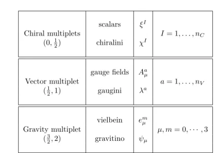
N = 1Supersymmetry N = 2 Supersymmetry

Chiral multiplet Hypermultiplet (0,1₂) (0,1₂,1₂,0)

Vector multiplet Vector multiplet (1

2,1) (0, 1 2,

1 2,1)

Gravity multiplet Gravity multiplet (3₂,2) (1,3₂,3₂,2)

Table 1.1– Massless supermultiplets of globally and locally supersymmetric models withN = 1andN = 2in 4 space-time dimensions. We denote the supermultiplets by the helicitysof the particles they involve: (s0, s0+1

2)forN = 1, and(s0, s0+ 1

2, s0+ 1

2, s0+ 1)forN = 2 supersymmetry.

and in particular should be treated as a quantum theory. Similarly to the other three interactions, gravity can be described as a gauge theory, where the symmetries that are gauged are space-time symmetries. The corresponding gauge group is the Poincar´e group, which involves space-time translations, rotations and boosts. In contrast with gauged internal symmetries, the gauge boson is a spin-2 field, thegraviton, which represents the gravitational field itself.

(31)

graviton. In supergravity theories the number of gravitinos is equal to the number of the supersymmetry generators, N. The different types of massless supermultiplets ofN = 1 andN = 2 supersymmetry are summarized in table 1.1.

Supergravity plays an important role in the construction of cosmological mod-els, since it describes the low energy regime of the most prominent theory of quantum gravity to date,String Theory.

1.2.5 String theory and the integration of heavy moduli.

In contrast with conventional quantum field theory, where the elementary particles are mathematical points, the fundamental entities in string theory are one-dimensional extended objects, namelythe strings (see [19]). The basic idea is that the elementary particles of the Standard Model would arise as oscillation modes of these fundamental strings. An appealing feature of string theory is that it involves a single fundamental parameter, the characteristic length of the stringsls, or the corresponding energy scaleEs= 1/ls. Any other quantity, such

as the strength of the interactions between strings, is field dependent.

Another remarkable property of superstring theories is that they predict the number of space-time dimensions. Indeed, for these theories to be consistent, the fundamental strings must live in a 10− or 11−dimensional space-time. So far there is no experimental evidence of extra dimensions, thus in order for string theory to describe the 4−dimensional world we experience, we must invoke a mechanism to hide the 6 or 7 extra dimensions. The most accepted solution is that the extra dimensions arecompactified on some internal manifold, so small that it remains invisible even at the largest energy scales, (the shortest length scales), tested with current accelerators.

Simple compactifications can be characterized by a single length scale4_, _l c,

or its associated energy scaleEc= 1/lc. Many results in string theory have been

derived in the limitEc Es, because, in this regime, the physics at the energy

scalesE Es admit an effective description in terms of 10 or 11 dimensional

supergravity. However, given the absence of evidence of extra dimensions, most of the proposed cosmological models assume the extra condition E Ec, so

that they can be described in the framework of 4-dimensional supergravity.

A common problem that has to be treated in all cosmological models derived from string compactifications is the presence of a large number of massless scalar fields, for which so far there is no observational evidence. In particular, this set of fields involves the moduli fields, which characterize the size and shape

(32)

1.3. Cosmic strings and other topological defects.

of the extra dimensions. The mechanisms to generate a potential that can stabilize the moduli have only been developed recently [20, 21]. This requires compactifying string theory in a new type of backgrounds,flux compactifications, which require the presence of D-branes5 _{wrapping the internal dimensions, and}

certain generalizations of the magnetic flux sourced be the branes.

In flux compactifications some of the moduli are stabilized at a high energy scale and decouple from the low energy effective theory. On the other hand, as we have mentioned before, it is phenomenologically appealing that supersymmetry remains unbroken at scales as low as 1 TeV, therefore the stabilization of these heavy fields has to leave supersymmetry unbroken. However, integrating out heavy scalars in such a way that the effective theory is still invariant under supersymmetry is not a trivial problem, the couplings between the light and heavy sectors have to satisfy certain conditions. Thus, it is important to characterize the type of couplings between the two sectors that allow for the supersymmetric integration of the heavy fields. This problem will be discussed in detail in chapter 3.

There are two situations where details of the decoupling of heavy moduli be-come important. The first one is in inflationary models derived from supergravity or superstrings with moduli stabilization. In these models the inflaton belongs to the light sector of the theory, and the slow roll conditions can be easily spoilt by its couplings to the heavy fields [22]. Thus the predictions of these models can only be trusted after having a precise characterization of the interactions between the inflationary and heavy sectors [23] (see also [24]). The second situa-tion is supersymmetry breaking. Since supersymmetry is not an exact symmetry of nature, any realistic cosmological model should involve the mechanism for su-persymmetry breaking. The breaking of susu-persymmetry in the light sector will affect the stability properties of the heavy fields that were integrated out. In par-ticular, if the heavy fields become unstable due to the supersymmetry breaking effects, the integration of heavy moduli no longer makes sense. This is especially relevant in string theory models describing late time accelerated expansion of the universe. We will come back to this problem in chapter 4.

1.3 Cosmic strings and other topological defects.

We continue this introductory chapter with a discussion about the formation of topological defects in the early universe and their cosmological implications, paying particular attention to cosmic strings.

(33)

-1.5 -1 -0.5 0.5 1 1.5Φ 0.2

0.4 0.6 0.8V!Φ"

-6 -4 -2 2 4 6 x

-1 -0.5 0.5 1 Φ!x"

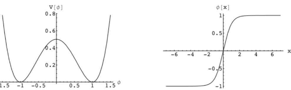
Figure 1.2 – The scalar potentialV(φ) in (1.3.2) (left) with λ= 2, η= 1 leads to the kink solution (1.3.4) φ(x)on the right.

As we have mentioned in the previous sections, phase transitions are a fundamental ingredient of many interesting cosmological scenarios, such as those based on Grand Unified Theories (GUT). An important example are hybrid inflationary models, where the exponential expansion ends in a natural way as the inflaton reaches a point of the potential with a tachyonic instability leading to a phase transition. Like in the more familiar condensed matter systems, phase transitions in the early universe also lead to the formation of localized, non-dissipative objects called topological defects (see [25, 26]). In particular, it has been proven that cosmological models based on Supersymmetric Grand Unified Theories generically predict the formation of cosmic strings at the end of inflation [27].

In this section we will introduce topological defects without considering the gravitational effects. In a theory without gravity, where the energy density is given by theT₀0component of the energy-momentum tensor (see [25]), the energy is bounded belowT00≥0 and the ground states satisfy T00= 0. We understand

bydissipative solutions of the classical equations of motion those satisfying:

lim

t→∞T

0 0(x

i_{, t}_{) = 0}_, _(1.3.1)

at every point of spacexi_.

The simplest example of a topological defect is the kink in 1 + 1 dimensions. It is possible to construct a model that exhibits kink solutions with a single real scalar fieldφ. The corresponding action is given by:

S = Z

dtdx−1 2∂µφ∂

µ_φ₋_V₍_φ₎

, (1.3.2)

where the potential is given byV(φ) =1 4λ(φ

2₋_η2₎2_{. The energy functional for}

this action reads:

E= Z

dx1 2(∂tφ)

2₊1 2(∂xφ)

2₊1 4λ(φ

2₋_η2₎2

(34)

In order for the solution to have a finite energy, the field configurationφdescribing the kink must satisfy φ2 = η2 at x → ±∞, it must be in one of the ground states of the potentialV(φ0) = 0. The set of ground states of a given theory is

called the vacuum manifold V, and in this case it is given by the homogeneous configurations φ0 =±η. Suppose now that we choose the boundary conditions

such thatφ(−∞) =−ηandφ(∞) =η, then by continuity this field configuration must necessarily have a zero for some value x=x0∈R. This configuration has

a nonzero energy, which is expected to be concentrated around x =x0, where

the scalar field is out of the vacuum. The kink solution to the classical equations of motion is given by:

φ(x) =ηtanh r

λ

2η(x−x0) !

, (1.3.4)

which is plotted in figure 1.2. This field configuration is non-dissipative in the sense that no classical time evolution can make this object decay into the vacuum

φ=±η. The reason is simple: for the energy to be finite, the value ofφat spatial infinity must remain in the vacuum manifold at all times. Since the vacuum man-ifold consists of two disconnected pieces, and time evolution is continuous, it is not possible for the scalar field to evolve to a constant field configurationφ=±η. This model provides an illustrative example of spontaneous breaking of a symmetry. Its lagrangian has a Z2 symmetry that exchanges φ and −φ.

When the Higgs condenses and chooses one of the vacua φ0 = ±η, the Z2

symmetry, which transforms the two vacua into each other, is spontaneously broken. In general, the vacuum manifold of a theory has a close relation with its underlying symmetry group G. Actually, since the scalar potential is invariant under the symmetry group, if φ0 is a zero of the potential so is gφ0 for any

transformation g ∈ G. Moreover, in the absence of accidental degeneracies, the vacuum manifold V can be identified with the coset space G/H, where H

is the unbroken subgroup. In the present case G = _Z2 is completely broken

(H ={ }), and therefore the vacuum manifold is isomorphic to the symmetry group itself V ∼=Z2. This discussion suggests that in the case of spontaneously

broken GUT theories the vacuum manifold can be highly non-trivial.

(35)

1.3.1 Global vortices.

The global U(1) model is the simplest field theory that exhibits cosmic string solutions. It describes the dynamics of a single complex scalar fieldφevolving in a scalar potential with a mexican hat form, fig. 1.3. The action reads:

S= Z

dx4

−∂µφ∂µφ¯−V(φ)

, V =λ(|φ|2₋_η2₎2_, _(1.3.5)

and its corresponding equation of motion is given by:

[∂µ∂µ−2λ(|φ|2−η2)]φ= 0. (1.3.6)

This model is invariant under a global U(1) symmetry defined by the transfor-mations:

φ→φ eigΛ, (1.3.7)

where Λ is a real constant. The energy functional associated to our action is:

E= Z

dx3

|∂tφ|2+|∂iφ¯|2+λ(|φ|2−η2)2

. (1.3.8)

As in the Abelian-Higgs model, this theory has a stable set of vacua given by all the configurations satisfying|φ| =η2, and therefore the vacuum manifold is isomorphic to a circle:

V ={φ∈C/|φ|2−η2= 0} ∼=S1. (1.3.9) Since these vacua are not invariant under the U(1) transformations (1.2.6), the global symmetry is said to be spontaneously broken down to the trivial group { }. The mass spectrum around the vacuum consists of two types of particles, one particle has a mass ms =

√

2λη, and the other is massless, the goldstone boson. The original U(1) symmetry of the action prevents the goldstone boson from having a mass, since this particle corresponds to the space dependent fluctuations of the phase of the scalar field.

This model admits cosmic string solutions, which are also known as global vortices. We will now discuss static cylindrically symmetric cosmic solutions laying along the z-axes. An appropriate ansatz for this configuration is given by:

φ=ηf(r)einθ, (1.3.10)

where we have used cylindrical coordinates{r, θ, z}. In order for the string con-figuration to have finite energy, the scalar field φ must approach the vacuum manifold asymptotically at spatial infinity, and thus the profile function f(r) must satisfy the boundary conditionf(r→ ∞) = 1. Therefore at spatial infinity the field configuration is

(36)

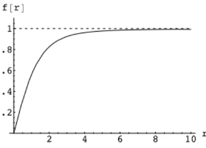
2 4 6 8 10 r 0.2

0.4 0.6 0.8 1 f!r"

Figure 1.3 – Profile function (1.3.10)f(r) =|φ(r)|characterizing the field con-figuration of a global string forn=λ=η= 1.

which represents a mapping between the the circle at infinity in real space and a circle in field space, the vacuum manifold. The parametern, called thewinding number, is an integer which counts the number of times the phase of the scalar field winds around the vacuum manifold when we go once around the circle in field space.

Since the field φ has to be single valued we have to require the profile functionf(r) to vanish at the originr = 0, thusφ leaves the vacuum manifold which implies that the field configuration has nonzero energy. Following the same argument we used in the case of the kink, we can see that there is no continuous way to deform the configuration 1.3.11 into a homogeneous solution of the form φ =eiα_{, and in particular, since time evolution is continuous, the}

cosmic string solution cannot decay into the vacuum.

Introducing the ansatz (1.3.10) into the equation of motion we obtain a second order ordinary differential equation for the profile functionf(r):

f00+_r12f

0₋n2

r2f+ 2λη

2₍₁₋_f2₎_f _{= 0}_. _(1.3.12)

The numerical solution of this equation is displayed in fig 2. The profile function

f(r) has the following asymptotic behavior:

f(r) ≈ Cnrn for r→0, (1.3.13)

f(r) ≈ 1− n

2

4λη2_r2 for r→ ∞. (1.3.14)

This indicates that the string core has a width of the order of the Compton wavelength of the massive scalar δ ∼ 1/(√2λη) = m−s1; for r equal to a few δ

(37)

energy functional (1.3.8). Including a small contribution from the core we obtain the following energy per unit lengthµ:

µ≈η2+ 2πn2η2

Z R

δ

dr r ≈2πn

2_η2_log_R/δ, _(1.3.15)

which is logarithmically divergent for large values of the cutoffR. In a cosmo-logical context this cutoff would be given by the distance to the nearest string with the opposite winding number. A characteristic property of these strings is that they interact with long range forces, which decay asR−1_{with the distance}

Rbetween them. Actually, due to the repulsion between the strings, those with winding number|n|>1 are unstable to decay into single |n|= 1 strings, which are completely stable [28].

1.3.2 Abrikosov-Nielsen-Olesen vortex.

Let us discuss again the Abelian-Higgs model presented in section 1.2.2. In this case the internal U(1) symmetry has been promoted to a local one. In our previous discussion of the Abelian-Higgs model we mentioned that the ground states of the system, up to gauge transformations, were given by the configurations satisfyingAµ= 0 andφ=ηeiα, withαsome real constant. Thus,

as in the global U(1) model, the vacuum manifold is isomorphic toS1, implying the existence of cosmic string solutions.

The cosmic strings in the Abelian-Higgs model have different properties from those in the global U(1) model. In particular it is possible to find solutions with finite energy per unit length. For the energy to be finite we have to require, as in the case of global vortices, the Higgs to lay in the vacuum manifold at spatial infinity:

lim |~x|→∞|φ|

2₌_η2_. _(1.3.16)

Moreover, the covariant derivativesDµφmust vanish asymptotically. In order to

achieve this the gauge fields have to satisfy the condition:

lim |~x|→∞Aµ=

1

ig∂µlogφ, (1.3.17)

which also implies that the field strengthFµν vanishes at spatial infinity, since

[Dµ, Dν]φ=−igFµνφ.

As in the previous section we now consider static cylindrically symmetric cosmic string solutions along the z-axis. We will use in cylindrical coordinates {r, θ, z}, and we will impose the gauge A0 = Ar = 0. A cosmic string with a

winding numberncan be described by the ansatz:

(38)

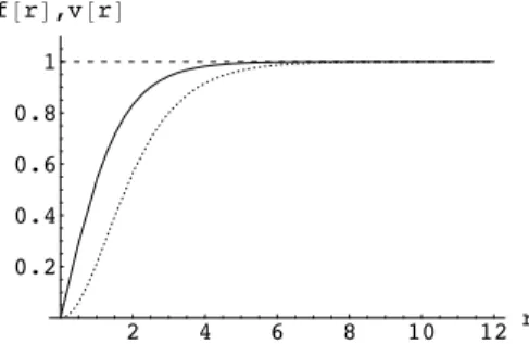
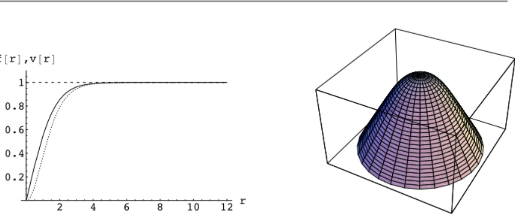
2 4 6 8 10 12r

0.2 0.4 0.6 0.8 1 f!r",v!r"

Figure 1.4 – Profile functions (1.3.18) f(r) (solid line) and v(r) (dotted line) characterizing the field configuration of a local string saturating the BPS bound,

2λ=g2, withn=g= 2η= 1.

where f(r) and v(r) are real functions satisfying the following boundary condi-tions:

f(r), v(r)→1 for r→ ∞, and f(r), v(r)→0 for r→0. (1.3.19) Introducing this ansatz in the equations of motion (1.2.3) we find the equations for the profile functionsf(r) andv(r):

f00(r) + 1_rf0(r)−n2

r2[1−v(r)]

2_{+ 2}_λη2₍₁₋_f₍_r₎2₎_f₍_r_{) = 0}_, _(1.3.20)

v00(r) − 1 rv

0₍_r_{) +}_g2_η2_[1₋_v₍_r_{)] = 0}_. _(1.3.21)

This type of vortices have a tube of magnetic flux in their core which is quantized by the winding number n. Integrating the magnetic flux over the whole plane perpendicular to the string gives:

Φm=

Z

R2

dx2B= Z

S1 ∞

d~l ~A=2πn

g . (1.3.22)

Here we have applied Stokes’ theorem withS_∞1 being the circle at spatial infinity containing the string, and used the the asymptotic behavior of the gauge field and the Higgs. The energy per unit length of these strings is finite and has a dependence on the parameters of the form [29]:

µ=πη2(2λ/g2). (1.3.23)

(39)

way:

µ = Z

dx2|(D1±iD2)φ|2+1₂[B±g(|φ|2−η2)]2+1₂(2λ−g2)(|φ|2−η2)2

±gη2

Z

d2xB≥0. (1.3.24)

This expression can be obtained from (1.2.5), using the identities:

|(D1±iD2)φ|2 = |Dφ~ |2∓i ¯φ[D1, D2]φ±∇ ∧~ J ,~ (1.3.25)

[D1, D2]φ = −igBφ, (1.3.26)

and discarding the boundary term associated to the curl of the currentJ~= i ¯φ ~∇φ. Note that in the limit 2λ=g2the first line in (1.3.24) is a sum of positive definite terms, and thus the energy per unit lengthµis bounded below6:

µ≥ ±gη2

Z

d2xB= 2πη2|n|. (1.3.27)

Any field configuration saturating this bound must also be a solution to the static equations of motion, since it extremizes the energy functional. In order to saturate the bound the cosmic string background must satisfy the following first order differential equations:

(D1±iD2)φ= 0, B±g(|φ|2−η2) = 0, (1.3.28)

which are know as the BPS equations. Inserting the ansatz for a cylindrically symmetric straight string (1.3.18) we obtain the following system of equations for the profile functions:

f0(r) +|n_r|(v(r)−1)f(r) = 0 |n|v0(r) +g2η2r(f(r)2−1) = 0. (1.3.29) These equations only admit solutions with the correct boundary conditions (1.3.19) provided we choose the signs so thatn=±|n|. The functionsf(r) and

v(r) which solve this set of equations are represented in figure 1.4. These cosmic strings have an energy per unit lengthµ=πη2_|_n_{|, which satisfies the expression}

(1.3.23) with= 1.

For generic values of the couplings, λand g, parallel cosmic strings interact with short-range forces. For instance, if 2λ > g2 _{the cosmic strings repel, and}

if 2λ < g2 _{they attract [30]. When the Abelian-Higgs model satisfies the BPS}

limit 2λ=g2_{, it is possible to find static multivortex solutions of the equations of}

motion [32]. In consequence, string configurations with windings|n|>1 are only stable provided that 2λ≤g2, otherwise the strings decay inton stable vortices with a unit of magnetic flux [28]. The vortex solutions of the AH model satisfying the BPS limit are especially interesting because their low energy dynamics can be studied with high accuracy using the moduli space approximation [33, 34, 35].

(40)

1.4. Topological defects in cosmology.

1.4 Topological defects in cosmology.

1.4.1 Defect formation.

The process of formation of topological defects in cosmology in known as the

Kibble mechanism [36] (for a review see [26]). As the universe undergoes a phase transition, in general the Higgs will condense into different vacua at different points in space time. For example in the model we just discussed, as the two vacuaφ=±η are completely equivalent from the point of view of the equations of motion, the Higgs could condense into any of them with equal probability. This leads to the formation of separate domains, or regions of the universe where the Higgs has the same value. As the universe cools down, these domains expand and eventually coalesce. In the boundary of the domains the scalar field interpolates between different vacua, as occurs in the previous example. These field configurations interpolating between different vacua at spatial infinity are the defects. The formation of these domains is unavoidable, because the vacuum where the Higgs condenses can only be correlated over finite distances smaller than the size of the horizon (see section 1.1), and therefore it will be different at points of space-time which are not in causal contact.

The type of topological defects that are formed during a phase transition is determined by the topology of the vacuum manifold. The value of the Higgs in a

m-sphereSmat spatial infinity defines a continuous maphbetweenSm andV:

h:Sm−→ V. (1.4.1)

Since the Higgs has to remain in the vacuum manifold at spatial infinity at all times, and time evolution is a continuous operation, then it is clear that the existence of stable defects can be determined studying the set of continuous deformations of the maph. In particular, non-dissipative solutions are associated with non-contractiblem-spheres in the vacuum manifold. Saying that the image of the the map h cannot be contracted to a point, is the same as stating that the field cannot evolve to a homogeneous configuration. Note that if the field configuration ”wraps around” one of these non-contractible m-spheres of the vacuum manifold, then continuity implies that somewhere in real space the Higgs must leave the vacuum manifold restoring the old (symmetric) phase. As in the case of the kink, the energy density is expected to peak in the region of space where the Higgs leaves the vacuum. These concentrations of energy signal the positions of the defects.

The non-contractiblem-spheres of the vacuum manifold are classified by the elements of the m-th homotopy group7 _π

m(V). In particular, if the vacuum

manifold is disconnected, π0(V)6= , sheet-like structures are formed:

topolog-ical domain walls. When the first homotopy group of the vacuum manifold is

7_{The set}_π

(41)

non-trivial then one-dimensional defects form during the transition: topological

cosmic strings. Ifπ2(V) is non trivial then the phase transition will lead to the

formation of point defects, topologicalmonopoles.

For example, in the case of vortices (both global and local), the gauge group

G = U(1) is completely broken by the vacuum, i.e. the unbroken subgroup

H = . Therefore the vacuum manifold has a non-trivial first homotopy group

π1(U(1)/ ) =π1(S1) =Z, implying that the action should admit cosmic string

solutions labeled by an integern∈_Z, which is precisely the winding number of the string.

1.4.2 Cosmological implications.

The formation of defects has many cosmological implications. In particular, in four dimensions, they contribute to the energy density of the universe, affecting its geometry and the evolution of the scale factor. They might source density perturbations in the CMB in addition to those seeded by inflation, and they can have an impact in the amount of observed dark matter. The predictions of cosmological models related to the formation of defects, when contrasted with astronomical data, can help to constrain their parameter space, or even rule them out completely.

Domain walls and magnetic monopoles are very constrained from the observations. Let’s consider first the case of a domain wall network. Although the expansion of the universe tends to dilute the density of the network, at the same time these sheet-like defects are stretched. Since their surface energy density remains constant, the energy density of the network evolves with the scale factor as ρdw ∼ a−1 rapidly dominating any other contribution, which

is in contradiction with the observations (1.1.6). The production of magnetic monopoles during the GUT transition leads to a similar problem. According to these theories magnetic monopoles would be created with high abundances and, moreover, since they are extremely massive,mmonop∼1016GeV, they would

be-have as non-relativistic matterρmonop∼a−3. Although, in principle, monopoles

and anti-monopoles can annihilate, the process is not effective enough to reduce their abundance significantly. Therefore in a standard Big-Bang cosmological scenario their formation would lead to an overclosed universe, and would also disrupt the Big-Bang nucleosynthesis. As we saw in section 1.1, this discrepancy with the astronomical data can be cured invoking a period of inflation after the GUT transition. After inflation monopoles become extremely rare, with only one per Hubble volume, and do not have significant cosmological implications.

(42)

produc-1.5. Cosmic Strings.

tion of small loops8. The numerical simulations of cosmic string formation show that generically the networks consist of a small number of infinite strings (∼10) crossing the Horizon, together with a scale invariant distribution of small loops. These loops are continuously formed during the self-interesctions of the long strings. Due to the tension of the string, the loops oscillate and shrink emitting gravitational waves. The network has an additional energy loss mechanism, namely the emission of massive radiation. Full field theory simulations indicate that the later one is the main energy loss mechanism [37, 38], while Nambu-Goto simulations seem to favor loop production [39]. According to a recent work by Blanco-Pilladoet al. [40] the origin of the discrepancies arises because most loops form in scales too large to fit in the simulation box9_{of field theory calculations,}

while Nambu-Goto simulations do not describe the emission of massive radiation.

Eventually, no matter which is the main energy mechanism, the network reaches a scaling regime, where all its relevant length scales grow in proportion with the size of the Horizon. It follows that during the scaling regime the energy density of the network evolves as ρstring ∼ µt−2, with µ the string tension,

similarly to the critical density ρc ∼G−1t−2. Therefore their quotient remains

a constant, which for GUT strings is of the order of Ωstring ∼Gµ∼10−6, and

does not contradict the observations.

1.5 Cosmic Strings.

The formation of a cosmic string network after inflation is a common prediction of many promising cosmological models (see [41, 42, 43]). In particular it was shown in [27] that all supersymmetric GUT scenarios below a certain complexity, (based in gauge groups with rank r ≤ 8), lead to the formation of cosmic strings. More recently, in the context of superstrings, string net-works have been proven to appear at the end of brane inflation10_{, which is a}

particular realization of hybrid inflationary models in the context of superstrings.

Cosmic strings were originally proposed in the 80’s as a possible candidate to explain the primordial perturbations observed in the CMB. Nowadays inflation, due to its remarkable prediction of the CMB spectrum, has been established as the main mechanism to seed the perturbations, but the CMB data is still compatible with a 4.8% contribution from cosmic strings11_[44].

8_{Global string networks lose energy in a very efficient way too. Due to the coupling to the} goldstone boson the strings can radiate their energy into massless particles.

9_{The size of the simulation box is limited by the computational resources available and the} complexity of the problem.

10_{In brane inflationary models the brane positions along the compact directions play the role} of the inflaton.

Consistent supersymmetric decoupling in cosmology

Cover Page

The handle http://hdl.handle.net/1887/19115 holds various files of this Leiden University

dissertation.

Author: Sousa Sánchez, Kepa

Consistent Supersymmetric

Decoupling in Cosmology.

Consistent Supersymmetric

Decoupling in Cosmology.

PROEFSCHRIFT

D

U

L

R

M

P

F

H

C

P

2012

Kepa Sousa S´

anchez

Promotiecommissie:

Contents

Preface

CHAPTER

1

Introduction: cosmological models

in field theory and topological

defects.

1.1

Cosmology

1.1.1

Cosmic Inflation.

1.2

High energy physics.

1.2.1

Symmetry and spontaneous symmetry breaking.

1.2.2

Spontaneous breaking of local symmetries,

the Abelian-Higs model.

1.2.3

The Standard Model and Grand Unification

Theo-ries.

1.2.4

Supersymmetry and supergravity.

1.2.5

String theory and the integration of heavy moduli.

1.3

Cosmic strings and other topological defects.

1.3.1

Global vortices.

1.3.2

Abrikosov-Nielsen-Olesen vortex.

1.4

Topological defects in cosmology.

1.4.1

Defect formation.

1.4.2

Cosmological implications.

1.5

Cosmic Strings.