Performance Characteristics Optimization of
Electrical Discharge Machining Process using
Back Propagation Neural Network
and Genetic Algorithm
Robert Napitupulu1, Arif Wahyudi1, and Bobby O.P Soepangkat1
AbstractThis study attempts to make a model and optimize the complicated Electrical Discharge Machining (EDM) process using soft computing techniques. Artificial Neural Network (ANN) with back propagation algorithm is used to model the process. In this study, the machining parameters, namely pulse current, on time, off time and gap voltage are optimized with considerations of multiple performance characteristics such as Metal Removal Rate (MRR) and surface roughness. As the output parameters are conflicting in nature so there is no single combination of cutting parameters, which provides the best machining performance. Genetic Algorithm (GA) with properly defined objective functions was then adapted to the neural network to determine the optimal multiple performance characteristics.
KeywordsElectrical discharge machining (EDM), Artificial neural network (ANN), Multiple performance characteristics, Genetic algorithm (GA).
AbstrakPada penelitian ini mencoba untuk membuat model dan mengoptimalkan proses yang rumit pada Electrical Discharge Machining (EDM) menggunakan teknik komputasi. Jaringan Saraf Tiruan (JST) dengan algoritma propagasi kembali digunakan untuk memodelkan proses. Dalam penelitian ini, parameter mesin, yaitu pulsa saat ini, tepat waktu, off waktu dan kesenjangan tegangan dioptimalkan dengan pertimbangan dari beberapa karakteristik kinerja seperti Metal Removal Rate (MRR) dan kekasaran permukaan. Sebagai parameter output bertentangan di alam sehingga tidak ada kombinasi tunggal parameter pemotongan, yang menyediakan kinerja mesin terbaik. Algoritma genetika (GA) dengan didefinisikan dengan baik fungsi obyektif kemudian disesuaikan dengan jaringan saraf untuk menentukan beberapa karakteristik kinerja yang optimal.
Kata KunciDistribusi Log-logistik, Momen, Kumulan, FungsiKarakteristik.
I.INTRODUCTION1
log-logistic Electrical Discharge Machining (EDM) is one of the most extensively used non-conventional material removal or machining process. The unique feature of this process is the usage of thermal energy to machine electrically conductive parts regardless of hardness. This characteristic has become the distinctive advantage of EDM process in the manufacture of mould, die, automotive, aerospace and surgical component [1]. The selection of machining parameters for obtaining optimal responses is very much essential as this is a costly process to increase production rate considerably by reducing the machining time.
Material Removal Rate (MRR), surface roughness and tool wear are the most important response parameters in die-sinking EDM. Several researchers have conducted various investigations for improving the process performance [2–7]. Determination of proper machining parameters for obtaining the best process performance is still a challenging job. To solve this type of multi-optimization problem Lin et al. [2] used Grey Relational Analysis (GRA) based on an orthogonal array and fuzzy based Taguchi method. Lin and Lin [3] used grey-fuzzy
1Robert Napitupulu, Arif Wahyudi, and Bobby O.P Soepangkat are
with Departement of Mechanical Engineering, Faculty of Industrial Technology, Institut Teknologi Sepuluh Nopember, Surabaya, 60111, Indonesia. Email: [email protected]; [email protected]; [email protected].
logic for the optimization of EDM sinking process, as the performance parameters are fuzzy in nature, such as higher the better (MRR) and lower the better (tool wear and surface roughness), and contain certain degree of uncertainty. Grey relational coefficient analyzes the relational degree of the multiple responses (material removal rate, surface roughness and electrode wear rate). Fuzzy logic is used to perform a fuzzy reasoning of the multiple performance characteristics.
Artificial Neural Networks (ANN) have been developed by using the current understanding of the biological nervous system, and considered to be highly flexible modeling tools with capabilities on learning the mathematical mapping between input variables and output features for nonlinear system [8]. The relationships between machining parameters of EDM such as current, pulse on time and pulse off time and MRR and tool wear have been developed by using Back Propagation Neural Network (BPNN) [9]. MRR model has also developed for EDM process using pulse on time, pulse off time, sparking frequency and gap current [10].
of the EDM parameters has been done by Su et al. [5] and conducted from the rough cutting to the finish cutting stage.The relationship between the machining parameters and machining performance was established by using a trained neural network. GA with properly defined objective functions was then adapted to the neural network to determine the optimal machining parameters. Transformation of MRR, tool wear and surface roughness into a single objective was conducted by using a simple weighted method.
EDM process has been considered as complex and stochastic process [9]. It is difficult to determine the optimal EDM parameters for best machining performance such as productivity and accuracy. MRR and tool wear are two important output parameters which decide the cutting performance. But these performance parameters are conflicting in nature. The characteristic of MRR is the higher is better while the characteristic of tool wear is lower is better.
In a single objective optimization, there is only one solution. But in case of multiple objectives, there may not exist one solution, which is the best with respect to all objectives. In EDM process, it is not easy to obtain a single optimal combination of machining parameters for the performance parameters, as the machining parameters affect them differently. Classical methods for solving multi-objective problem have some drawbacks. Hence, there is a need for a multi-objective optimization method to arrive at the solutions to this problem. These methods transform the multi-objective problem into single objective by assigning some weights based on their relative importance [9]. These classical methods will also fail when the function becomes discontinuous.
Since GA is a good tool for solving multi-objective optimization and its works with a population of points, it seems natural to use multi-objective GA in EDM process to determine the optimal solution point from best performance to capture a number of solutions simultaneously [11]. In the present work, a hybrid of BPNN and GA has been used to obtain the optimal combination of machining parameters.
II.METHOD Material and Equipments
In this study, an EDM machine Hitachi H-DS025 was used as the experimental machine. A rectangular copper was used as electrode to erode a workpiece of AISI 4140 with a diameter of 25 mm. The schematic diagram of the experimental set-up is shown in Fig. 1. The w orkpiece and electrode were separated by a moving dielectric fluid such as kerosene.
Artificial Neural Network (ANN)
An ANN can be briefly described as an information-processing system that has certain performance characteristics in common with biological neural networks. According to Thillaivannan et al. [11], ANN have been developed as generalization of mathematical models of human cognition or neural biology based on the assumptions that:
a. The processing of information occurs at many elements called neurons.
b. Signals are passed between neurons over connection links.
c. Each connection link has an associated weight, which, in a typical neural net, multiplies the signal transmitted.
d. An activation function (usually nonlinear) is applied by each neuron to its net input (sum of weighted input signals) to determine its output signal.
There are numerous studies that have been reported on the development of neural networks based on different architectures in the past decades. Basically, neural networks can be characterized by its important features, such as the architecture, the activation functions, and the learning algorithms. In general, each category of the neural networks would have its own input characteristics, and therefore it can only be applied for modeling some specific processes [11].
1) Architecture
In general, neural networks are categorized by their architecture. The convergence rate at the stage of training the network parameters is determined by the number of hiddeen layers. Since the number of neurons is typically assumed to be dominant in the networks, one hidden layer could be considered sufficient in the multi-layered networks. Hence, the number of neurons must be determined by an optimization method [11]. MATLAB® software, which is a high-performance language for technical computing, can be used for modeling and developing of neural network.
2) Activation Functions
Signal links designated by corresponding weightings are used to connect the neurons. An internal state called the activation is representing each individual neuron. The activation is functionally dependent of the inputs. The sigmoid functions (S-shaped curves), such as logistic functions and hyperbolic tangent functions, are generally adopted for representing the activation. In the networks, a neuron sends its activation to the other neurons for information exchange via signal links [11].
3) Algorithm
There are numerous variations of the backpropagation algorithm. The simplest implementation of backpropagation learning updates the network weights and biases in the direction in which the performance function decreases most rapidly the negative of the gradient. One iteration of this algorithm can be written as Xk+1 = Xk – αk gk
where Xk+1 is a vector of current weights and biases, Xk is the current gradient, and gk is the learning rate.
This algorithm can be implemented in two different ways, namely incremental mode and batch mode. In the incremental mode, the gradient is computed and the weights are updated after each input is applied to the network. In the batch mode all of the inputs are applied to the network before the weights are updated [11].
4) Training
performance of the standard steepest descent algorithm. One heuristic modification is the momentum technique. There are two more heuristic techniques, i.e., variable learning rate backpropagation and resilient backpropagation.
5) Backpropagation
There are several applications of ANN such as Back-Propagation Network (BPN) and a General Regression Neural Network (GRNN). In general, BPN can be considered as the most utilized neural network. The development of BPN represents a landmark in the history of neural networks because it provides a computationally efficient method for the training of the multi-layer perceptron [12]. A multi-layer perceptron trained with the back propagation algorithm may be viewed as a practical way of performing a non-linear input-output mapping of a general nature.
Genetic Algorithm
The development of GA was based on the probabilistic nature that the global optimum is searched in a random and parallel manner through operations of reproduction, crossover and mutation [13]. Many conventional optimization methods have the disadvantage of requiring derivatives of an objective function about the problem to be solved and become easily trapped into local minimum in the search scope [13].
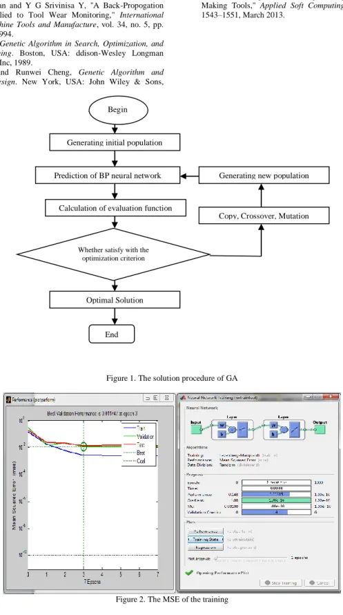
There are three main operators in GA, i.e., selection, crossover and mutation [14]. Selection means that two individuals from the whole population of individuals are selected as “parents.” Crossover serves to exchange the segments of selected parents between each other according to a certain probability. In other words, it combines two parents to form children for the next generation. The mutation operation randomly alternates the value of each element in a given chromosome according to the mutation probability. Mutation forms new children at random so as to avoid premature convergence. The procedure may be stopped after the terminated condition has been reached. Fig.2 illustrates the solution procedure of GA.
III.RESULT AND DISCUSSION
An experiment was designed using Taguchi method [15], which uses an orthogonal array to study the entire parametric space with a limited number of experiments. The four EDM parameters (control factors) are pulse current, on time, off time and gap voltage. As shown in Table 1, one of them was set at two different levels while the other three were set at three different levels. Therefore, the total degrees of freedom were seven. L18
orthogonal array that used for the experiment is shown in Table 2 and led to a total 18 tests. A random order was also determined for running the tests.
Transformation Data
The data that would be used for input layer and output layer of the BPNN should be transformed in accordance with the interval of activation function. In this study, the sigmoid biner (logsig) and sigmoid bipolar (tansig) functions are adopted for representing the activation. Based on the sigmoid biner activation, the data should be in the interv al of [0,1]. But, the value of the data according to this activation function are greater than 0 or
less than 1. Hence, the data are transformed into the interval of [0.1,0.9] [16]. The transformation is also conducted based on the quality characteristics of the responses.
Since the quality characteristic of MRR (larger is better) is opposite of the quality characteristic of surface roughness (smaller is better), the transformation of the input parameters (pulse current, on time, off time and gap voltage) and surface roughness are conducted by using the following equation:
(𝑘) = 0.1 + 0.8 𝑋𝑖(𝑘)−min 𝑋𝑖(𝑘)
max 𝑋𝑖(𝑘)− min 𝑋𝑖(𝑘) (1) 𝑋𝑖∗(𝑘) is the transformed values of machining
parameters and responses. Min 𝑋𝑖(𝑘) is the smallest
value of 𝑋𝑖(𝑘) for the kth response and max 𝑋𝑖(𝑘) is the
largest value of 𝑋𝑖(𝑘) for the kth response.
Table 3 shows the result of the transformation of each
input parameters, MRR and surface roughness which would be used as the input and output parameters in developing BPNN based prediction model. In this study, MATLAB version R210a is used as a computing software.
1) Architecture of BPNN
In this study, the varied parameters or factors for developing BPNN are:
a. The number of hidden layer: 1 and 2.
b. The number of neuron in each hidden layer: 8 and 10. c. Activation function: logsig and tansig.
d. Training method: trainlm and trainrp.
An experiment using 24 full factorial design is
conducted to determine the combination of parameters or factors which which could give the smallest Mean Square Error (MSE). Table 4 shows 16 combinations of parameters used to develop BPNN network. This experiment uses learning rate 0.1 and the performance goal is 1e-10.
2) Training, Testing and Validation
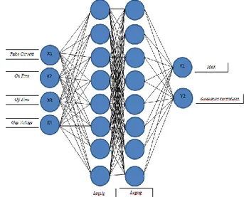
Generally, in developing the prediction model based on BPNN, the percentages of the data used for training, testing and validation are 70%, 15% and 15% respectively. Figure 3 shows the MSE of the training using the first network which consists of eight neurons, one hidden layer, logsig type of activation function and trainlm type of training function. The output type is purelin. The MSE obtained after training 16 networks are shown in Figure 4. The sixth network of the network architecture 4-8-8-2 with logsig activation function and trainrp training type has the smallest value of MSE, i.e., 0.00852. Network architecture 4-8-8-2 implies 4-input layer, 2-hidden layer with 8 neurons in each hidden layer and 2-output layer, and shown in Fig. 5.
3) Optimization of GA-based BPNN (GA-BPNN)
The setting parameters of optimization are as follows: a. Population size = 500
b. Crossover probability = 0.6 c. Generation = 60
d. Mutation probability = 0.05 e. Initial = [0;1]
Optimization for obtaining maximum MRR and minimum surface roughness is conducted by using the following steps:
Table 3 shows that values of MRR and surface roughness of the 10th combination of machining
parameters are 0.3634 and 0.141 respectively. Hence, the least average value of MRR and surface roughness can be calculated as follows:
𝑀𝑒𝑎𝑛 = 𝐴𝑣𝑒𝑟𝑎𝑔𝑒 𝑀𝑅𝑅+𝑎𝑣𝑒𝑟𝑎𝑔𝑒 𝑠𝑢𝑟𝑓𝑎𝑐𝑒 𝑟𝑜𝑢𝑔ℎ𝑛𝑒𝑠𝑠
2 (2) 𝑀𝑒𝑎𝑛 = 0.3634 + 0.141
2 𝑀𝑒𝑎𝑛 = 0.2520
Enter the above value into MATLAB software version R2010a.
1. Run the program which would be terminated if: a. The total number of generation (60) or maximum
iteration has been achieved.
b. The best fitness value has been achieved.
The result shows that the average value of MRR and surface roughness of the 348th combination of machining
parameters is 0.1489, lower than the initial value of the average of MRR and surface roughness, i.e., 0.2520. Table 5 shows the result of the GA-BPNN optimization of MRR and surface roughness.
4) Verification
Verification experiment is conducted by using the combination of the machining parameters resulted from GA-BPNN as shown in Table 6 with five replications. The result of the verification experiment then compared to the result of the 10th combination of machining
parameters of the initial experiment. Table 7 shows the comparison of the results of verification experiment and initial experiment.
Table 7 shows that the average of MRR and surface roughness resulted by the verification experiment (0.136) is lower than the average of MRR and surface roughness resulted by the initial experiment (0.252). This result has proven that the optimum setting of EDM sinking
machining parameters could give a better MRR and surface roughness than the initial setting.
Two-sample t-test is conducted to determine whether the MRR of verification experiment is larger than the MRR of initial experiment, and the surface roughness of verification experiment is smaller than the surface roughness of initial experiment. The followings are the hypothesis of the statistical tests for:
a. MRR
H0: The average of MRR of initial experiment = the
average of MRR of verification experiment
H1: The average of MRR of initial experiment < the
average of MRR of verification experiment b. Surface roughness
H0: The average of surface roughness of initial
experiment = the average of surface roughness of verification experiment
H1: The average of surface roughness of initial
experiment > the average of surface roughness of verification experiment.
The results of the two-sample t-test are shown in Table 8. The optimum setting of the EDM sinking machining parameters resulted from the BPNN-GA optimization is gap voltage at 9 volt, off time at 21 µs s, on time at 50 µs and pulse current at 25 ampere. The result of the hypothesis test of MRR concludes that the average of MRR of initial experiment is the same with the average
of MRR of verification experiment. Table 9 shows that the optimum setting of EDM sinking machining parameters produces more precise values of MRR than the initial setting. Therefore, even though those two averages are statistically the same, it can be concluded that the optimum setting would produce a higher MRR. As shown in Table 9, MRR is increased from 19.5 to 27.077 mm3/min and SR is decreased from 2.51 to 2.25
µm.
CONCLUSION
The paper has presented the use of the combination of Back Propagation Neural Network (BPNN) and Genetic Algorithm (GA) for the optimization of EDM sinking process with multiple performance characteristics. A verification experiment has been conducted to confirm the results of this approach. As a result, the optimization methodology developed in this study is useful in improving multiple performance characteristics in the EDM sinking process. The setting of the EDM sinking parameters which produce the maximum MRR and the lowest surface roughness is gap voltage at 9 volt, off time at 21 µs s, on time at 50 µs and pulse current at 25 ampere.
REFERENCES
[1] Shankar Singh, S Maheshwari, and P C Pandey, "Some Investigations into The Electric Discharge Machining of Hardened Tool Steel using Different Electrode Materials," Journal of Material Processing Technology, vol. 149, no. 1-3, pp. 272–277, June 2004.
[2] C L Lin, J L Lin, and T C Ko, "Optimisation of The EDM Process Based on The Orthogonal Array with Fuzzy Logic and Grey Relational Analysis Method," International Journal of Advanced Manufacturing Technology, vol. 19, no. 4, pp. 271– 277, February 2002.
[3] J L Lin and C L Lin, "The use of Grey-Fuzzy Logic for The Optimization of The Manufacturing Process," Journal of Materials Processing Technology, vol. 160, no. 1, pp. 9–14, March 2005.
[4] Kesheng Wang, Hirpa L Gelgele, Yi Wang, Qingfeng Yuan, and Minglung Fang, "A Hybrid Intelligent Method for Modelling The EDM Process," International Journal of Machine Tools and Manufacture, vol. 43, no. 10, pp. 995–999, August 2003. [5] J C Su, J K Kao, and Y S Tarng, "Optimisation of The Electrical
Discharge Machining Process using a GA-Based Neural Network," The International Journal of Advanced Manufacturing Technology, vol. 24, no. 1, p. July, July 2004.
[6] Shajan Kuriakose and M S Shunmugam, "Multi-objective Optimization of Wireelectro Discharge Machining Process by Non-Dominated Sorting Genetic Algorithm," Journal of Materials Processing Technology, vol. 170, no. 1-2, pp. 133– 141, December 2005.
[7] Cao Fenggou and Yang Dayong, "The Study of High Efficiency and intelligent Optimization System in EDM Sinking Process," Journal of Materials Processing Technology, vol. 149, no. 1-3, pp. 83–87, June 2004.
[8] Jun Qu and Albert J Shih, "Development of The Cylindrical Wire Electrical Discharge Machining Process, Part I: Concept, Design, and Material Removal Rate," Journal of Manufacturing Science and Engineering, vol. 124, pp. 237-244, August 2002.
[9] Debabrata Mandal, Surjya K Pal, and Partha Saha, "Modeling of Electrical Discharge Machining Process using Back Propagation Neural Network and Multi-Objective Optimization using Non-Dominating Sorting Genetic Algorithm-II," Journal of Materials Processing Technology, vol. 186, no. 1-3, pp. 154–162, May 2007.
[11] A Thillaivanan, P Asokan, K N Srinivasan, and R Saravanan, "Optimization of Operating Parameters for EDM Process Based on The Taguchi Method and Artificial Neural Network," Int. Journal of Engineering Science and Technology, vol. 2, no. 12, pp. 6880-6888, 2010.
[12] S Purushothaman and Y G Srivinisa Y, "A Back-Propogation Algorithm Applied to Tool Wear Monitoring," International Journal of Machine Tools and Manufacture, vol. 34, no. 5, pp. 625–631, July 1994.
[13] D E Goldberg, Genetic Algorithm in Search, Optimization, and Machine Learning. Boston, USA: ddison-Wesley Longman Publishing Co., Inc, 1989.
[14] Mitsuo Gen and Runwei Cheng, Genetic Algorithm and Engineering Design. New York, USA: John Wiley & Sons, 1997.
[15] S H Park, Robust Design and Analysis for Quality Engineering, 1st ed.: Springer, 1996.
[16] C Ahilan, Somasundaram Kumanan, N Sivakumaran, and J Edwin R Dhas, "Modeling and Prediction of Machining Quality in CNC Turning Process using Intelligent Hybrid Decision Making Tools," Applied Soft Computing, vol. 13, no. 3, pp. 1543–1551, March 2013.
Figure 1. The solution procedure of GA
Figure 2. The MSE of the training Beg
in
Generating initial population
Prediction of BP neural network
Calculation of evaluation function
Copy, Crossover, Mutation Generating new population
Optimal Solution Whether satisfy with the
optimization criterion
Figure 3. The MSE after training 16 networks Figure 5. BPNN network architecture used for modeling.
TABLE 1.
MACHINING PARAMETERS AND THEIR LEVELS
TABLE 2. ORTHOGONAL ARRAY L18
Run Order
Machining Parameters
Gap voltage
(Volt)
Off time (µs)
On time (µs)
Pulse Current (Ampere)
1 8 21 50 15
2 8 23 100 15
3 8 25 150 15
4 8 21 50 20
5 8 23 100 20
6 8 25 150 20
7 8 21 50 25
8 8 23 100 25
9 8 25 150 25
10 10 21 50 15
11 10 23 100 15
12 10 25 150 15
13 10 21 50 20
14 10 23 100 20
15 10 25 150 20
16 10 21 50 25
17 10 23 100 25
18 10 25 150 25
0.000000 0.001000 0.002000 0.003000 0.004000 0.005000 0.006000 0.007000 0.008000 0.009000 0.010000 0.011000 0.012000 0.013000 0.014000 0.015000 0.016000 0.017000 0.018000 0.019000 0.020000 0.021000 0.022000 0.023000 0.024000 0.025000 0.026000 0.027000 0.028000 0.029000 0.030000 0.031000 0.032000
1 3 5 7 9 11 13 15
Machining Parameters level 1 level 2 level 3
A Gap voltage (GV) Volt 8 - 10
B Off time (OFF) s 21 23 25
C On time (ON) s 50 100 150
TABLE 3.
THE RESULT OF THE TRANSFORMATION OF EACH INPUT PARAMETERS
TABLE 4.
COMBINATIONS OF PARAMETERS USED TO DEVELOP BPNN NETWORK.
Network Neuron
Unit
Hidden Layer
Activation function
Training function
1 8 1 logsig trainlm
2 8 1 logsig trainrp
3 8 1 tansig trainlm
4 8 1 tansig trainrp
5 8 2 logsig trainlm
6 8 2 logsig trainrp
7 8 2 tansig trainlm
8 8 2 tansig trainrp
9 10 1 logsig trainlm
10 10 1 logsig trainrp
11 10 1 tansig trainlm
12 10 1 tansig trainrp
13 10 2 logsig trainlm
14 10 2 logsig trainrp
15 10 2 tansig trainlm
16 10 2 tansig trainrp
TABLE 5.
THE RESULT OF THE GA-BPNN OPTIMIZATION OF MRR AND SURFACE ROUGHNESS.
Combination of machining parameters
Machining Parameters Responses
Gap Voltage (V) Off Time (µs) On Time (µs) Pulse Current
(A)
MRR (mm3/min)
Surface Rouhness
(µm)
348 0.42695 0.10334 0.17831 0.89976 0.16457 0.13339
348 88.174 213.916 504.178 249.971 34.135 48.551
348 9 21 50 25 34.135 48.551
Run Gap
Voltage Off Time
On Time
Pulse
Current MRR
Surface Roughness
Run Gap
Voltage Off Time
On Time
Pulse
Current MRR
Surface Roughness
Order Order
1 0.100 0.100 0.100 0.100 0.8809 0.1290 1 0.100 0.100 0.100 0.100 0.9 0.142
2 0.100 0.100 0.500 0.500 0.6358 0.3310 2 0.100 0.100 0.500 0.500 0.6606 0.321
3 0.100 0.100 0.900 0.900 0.3908 0.3660 3 0.100 0.100 0.900 0.900 0.5183 0.492
4 0.100 0.500 0.100 0.100 0.7516 0.3930 4 0.100 0.500 0.100 0.100 0.7911 0.217
5 0.100 0.500 0.500 0.500 0.6386 0.5200 5 0.100 0.500 0.500 0.500 0.5959 0.4
6 0.100 0.500 0.900 0.900 0.2895 0.6240 6 0.100 0.500 0.900 0.900 0.3726 0.601
7 0.100 0.900 0.100 0.500 0.5529 0.4920 7 0.100 0.900 0.100 0.500 0.6181 0.443
8 0.100 0.900 0.500 0.900 0.3506 0.4470 8 0.100 0.900 0.500 0.900 0.4477 0.422
9 0.100 0.900 0.900 0.100 0.7859 0.4000 9 0.100 0.900 0.900 0.100 0.7784 0.549
10 0.900 0.100 0.100 0.900 0.4526 0.1180 10 0.900 0.100 0.100 0.900 0.2741 0.163
11 0.900 0.100 0.500 0.100 0.7858 0.1000 11 0.900 0.100 0.500 0.100 0.6088 0.202
12 0.900 0.100 0.900 0.500 0.4973 0.3380 12 0.900 0.100 0.900 0.500 0.6163 0.289
13 0.900 0.500 0.100 0.500 0.502 0.1700 13 0.900 0.500 0.100 0.500 0.4839 0.389
14 0.900 0.500 0.500 0.900 0.4075 0.5200 14 0.900 0.500 0.500 0.900 0.1966 0.396
15 0.900 0.500 0.900 0.100 0.7093 0.3330 15 0.900 0.500 0.900 0.100 0.7475 0.421
16 0.900 0.900 0.100 0.900 0.3676 0.2800 16 0.900 0.900 0.100 0.900 0.1 0.367
17 0.900 0.900 0.500 0.100 0.7527 0.2740 17 0.900 0.900 0.500 0.100 0.8447 0.221
TABLE 6.
THE RESULT OF THE VERIFICATION EXPERIMENT
Machining Parameters Responses
Gap Voltage
(V)
Off Time
(µs)
On Time (µs)
Pulse Current
(A)
MRR (mm3/min) Surface Roughness
(µm)
9 21 50 25
34.116 4.56
34.124 4.52
34.151 4.54
34.132 4.82
34.118 4.70
Average 34.128 4.63
TABLE 7.
THE RESULT OF THE VERIFICATION EXPERIMENT
Responses Transformed Responses
Average MRR (mm3/min)
Surface
roughness (µm) MRR (mm3/min)
Surface roughness (µm)
Verification 34.116 4.56 0.1652 0.100 0.133
experiment 34.124 4.52 0.1649 0.095 0.130
34.151 4.54 0.1641 0.098 0.131
34.132 4.82 0.1647 0.130 0.147
34.118 4.70 0.1651 0.116 0.141
Average 34.1282 4.628 0.1648 0.1078 0.136
Initial experiment
24.45 4.72 0.453 0.118 0.285
30.45 5.12 0.274 0.163 0.219
Average 27.45 4.92 0.3635 0.1405 0.252
TABLE 8.
THE RESULT OF THE TRANSFORMATION OF EACH INPUT PARAMETERS
Responses p-value H0 Average
MRR 0.866 Fail to reject μ1 = μ2
Surface roughness 0.048 Rejected μ1 > μ2
TABLE 9.
THE COMPARISON OF THE RESULTS OF VERIFICATION EXPERIMENT AND INITIAL EXPERIMENT.
Initial Optimal Process Condition
Improvement Prediction Verification
Level of machining parameters
GV (10 volt) GV (9 volt) GV (9 volt)
OFF (21 µs) OFF (21 µs) OFF (21 µs)
ON (50 µs) ON (50 µs) ON (50 µs)
PC (25 ampere) PC (25 ampere) PC (25 ampere)
Material Removal Rate
(mm3/min) 27.45 41.13 increased 24.33 %
Surface Roughness