IOS Press
RDF2Vec: RDF Graph Embeddings
and Their Applications
Editor(s):Freddy Lecue, Accenture Tech Labs, Ireland and INRIA, France
Solicited review(s):Achim Rettinger, Karlsruhe Institute of Technology, Germany; Jiewen Wu, Institute for Infocomm Research, Singapore;
one anonymous reviewer
Petar Ristoski
a, Jessica Rosati
b,c, Tommaso Di Noia
b, Renato De Leone
c, Heiko Paulheim
aaData and Web Science Group, University of Mannheim, B6, 26, 68159 Mannheim
E-mail: petar.ristoski@informatik.uni-mannheim.de, heiko@informatik.uni-mannheim.de
bPolytechnic University of Bari, Via Orabona, 4, 70125 Bari
E-mail: jessica.rosati@poliba.it, tommaso.dinoia@poliba.it
cUniversity of Camerino, Piazza Cavour 19/f, 62032 Camerino
E-mail: jessica.rosati@unicam.it, renato.deleone@unicam.it
Abstract.Linked Open Data has been recognized as a valuable source for background information in many data mining and information retrieval tasks. However, most of the existing tools require features in propositional form, i.e., a vector of nominal or numerical features associated with an instance, while Linked Open Data sources are graphs by nature. In this paper, we present RDF2Vec, an approach that uses language modeling approaches for unsupervised feature extraction from sequences of words, and adapts them to RDF graphs. We generate sequences by leveraging local information from graph sub-structures, harvested by Weisfeiler-Lehman Subtree RDF Graph Kernels and graph walks, and learn latent numerical representations of entities in RDF graphs. We evaluate our approach on three different tasks: (i) standard machine learning tasks, (ii) entity and document modeling, and (iii) content-based recommender systems. The evaluation shows that the proposed entity embeddings outperform existing techniques, and that pre-computed feature vector representations of general knowledge graphs such as DBpedia and Wikidata can be easily reused for different tasks.
Keywords: Graph Embeddings, Linked Open Data, Data Mining, Document Semantic Similarity, Entity Relatedness, Recommender Systems
1. Introduction
Since its introduction, the Linked Open Data (LOD)
[79] initiative has played a leading role in the rise of
a new breed of open and interlinked knowledge bases
freely accessible on the Web, each of them being part
of a huge decentralized data space, the LOD cloud.
This latter is implemented as an open, interlinked
col-lection of datasets provided in machine-interpretable
form, mainly built on top ofWorld Wide Web
Consor-tium(W3C) standards, such as RDF1 and SPARQL2. Currently, the LOD cloud consists of about1,000 in-terlinked datasets covering multiple domains from life science to government data [79]. The LOD cloud has been recognized as a valuable source of background knowledge in data mining and knowledge discovery in general [74], as well as for information retrieval and recommender systems [17]. Augmenting a dataset with background knowledge from Linked Open Data
1http://www.w3.org/TR/2004/
REC-rdf-concepts-20040210/, 2004.
2http://www.w3.org/TR/rdf-sparql-query/, 2008
can, in many cases, improve the results of the prob-lem at hand, while externalizing the cost of maintain-ing that background knowledge [61].
Most data mining algorithms work with a proposi-tionalfeature vectorrepresentation of the data, which means that each instance is represented as a vector of featureshf1, f2, ..., fni, where the features are ei-ther binary (i.e.,fi ∈ {true, f alse}), numerical (i.e.,
fi∈R), or nominal (i.e.,fi∈S, whereSis a finite set of symbols). Linked Open Data, however, comes in the form ofgraphs, connecting resources with types and relations, backed by a schema or ontology. Therefore, in order to make LOD accessible to existing data min-ing tools, an initialpropositionalization[34] of the cor-responding graph is required. Even though the new set of propositional features do not encode all the knowl-edge available in the original ontological data, they can be effectively used to train a model via machine learn-ing techniques and algorithms. Usually, binary features (e.g.,trueif a type or relation exists,false other-wise) or numerical features (e.g., counting the number of relations of a certain type) are used [63,72]. Other variants, e.g., counting different graph sub-structures, have also been proposed and used [91].
Typically, those strategies led to high-dimensional, sparse datasets, which cause problems for many data mining algorithms [1]. Therefore, dense, lower-dimensional representations are usually preferred, but less straight forward to generate.
In language modeling, vector space word embed-dings have been proposed in 2013 by Mikolov et al. [41,42]. They train neural networks for creating a low-dimensional, dense representation of words, which show two essential properties: (a) similar words are close in the vector space, and (b) relations between pairs of words can be represented as vectors as well, allowing for arithmetic operations in the vector space. In this work, we adapt those language modeling ap-proaches for creating a latent representation of entities in RDF graphs.
Since language modeling techniques work on sen-tences, we first convert the graph into a set of se-quences of entities using two different approaches, i.e., graph walks and Weisfeiler-Lehman Subtree RDF graph kernels. In the second step, we use those se-quences to train a neural language model, which esti-mates the likelihood of a sequence of entities appear-ing in a graph. Once the trainappear-ing is finished, each en-tity in the graph is represented as a vector of latent nu-merical features. We show that the properties of word
embeddings also hold for RDF entity embeddings, and that they can be exploited for various tasks.
We use several RDF graphs to show that such latent representation of entities have high relevance for dif-ferent data mining and information retrieval tasks. The generation of the entities’ vectors is task and dataset in-dependent, i.e., we show that once the vectors are gen-erated, they can be reused for machine learning tasks, like classification and regression, entity and document modeling, and to estimate the proximity of items for content-based or hybrid recommender systems. Fur-thermore, since all entities are represented in a low di-mensional feature space, building the learning models and algorithms becomes more efficient. To foster the reuse of the created feature sets, we provide the vec-tor representations of DBpedia and Wikidata entities as ready-to-use files for download.
This paper considerably extends [73], in which we introduced RDF2Vec for the first time. In particular, we demonstrate the versatility of RDF embeddings by extending the experiments to a larger variety of tasks: we show that the vector embeddings not only can be used in machine learning tasks, but also for document modeling and recommender systems, without a need to retrain the embedding models. In addition, we ex-tend the evaluation section for the machine learning tasks by comparing our proposed approach to some of the state-of-the-art graph embeddings, which have not been used for the specified tasks before. In further sets of experiments, we compare our approach to the state-of-the-art entity relatedness and document mod-eling approaches, as well to the state-of-the-art graph embedding approaches.
Preliminary results for the recommender task have already been published in [76]. In this paper, we fur-ther extend the evaluation in recommendation scenar-ios by considering a new dataset (Last.FM) and by implementing a hybrid approach based on Factoriza-tion Machines. Both contribuFactoriza-tions highlight the effec-tiveness of RDF2Vec in building recommendation en-gines that overcame state of the art hybrid approaches in terms of accuracy also when dealing with very sparse datasets (as is the case ofLast.FM).
2. Related Work
While the representation of RDF as vectors in an embedding space itself is a considerably new area of research, there is a larger body of related work in the three application areas discussed in this paper, i.e., the use of LOD in data mining, in document modeling, and in content-based recommender systems.
Generally, our work is closely related to the ap-proaches DeepWalk [65] and Deep Graph Kernels [95]. DeepWalk uses language modeling approaches to learn social representations of vertices of graphs by modeling short random-walks on large social graphs, like BlogCatalog, Flickr, and YouTube. The Deep Graph Kernel approach extends the DeepWalk ap-proach by modeling graph substructures, like graphlets, instead of random walks. Node2vec [22] is another ap-proach very similar to DeepWalk, which uses second order random walks to preserve the network neighbor-hood of the nodes. The approach we propose in this paper differs from these approaches in several aspects. First, we adapt the language modeling approaches on directed labeled RDF graphs, unlike the approaches mentioned above, which work on undirected graphs. Second, we show that task-independent entity vectors can be generated on large-scale knowledge graphs, which later can be reused on a variety of machine learning tasks on different datasets.
2.1. LOD in Machine Learning
In the recent past, a few approaches for generat-ing data mingenerat-ing features from Linked Open Data have been proposed. Many of those approaches assume a manual design of the procedure for feature selection and, in most cases, this procedure results in the formu-lation of a SPARQL query by the user. LiDDM [48] al-lows the users to declare SPARQL queries for retriev-ing features from LOD that can be used in different machine learning techniques. Similarly, Cheng et al. [10] proposes an approach for automated feature gen-eration after the user has specified the type of features in the form of custom SPARQL queries.
A similar approach has been used in the Rapid-Miner3semweb plugin [31], which preprocesses RDF data in a way that can be further handled directly in RapidMiner. Mynarz et al. [47] have considered using user specified SPARQL queries in combination with
3http://www.rapidminer.com/
SPARQL aggregates. FeGeLOD[63] and its succes-sor, theRapidMiner Linked Open Data Extension[70], have been the first fully automatic unsupervised ap-proach for enriching data with features that are derived from LOD. The approach uses six different unsuper-vised feature generation strategies, exploring specific or generic relations. It has been shown that such fea-ture generation strategies can be used in many data mining tasks [64,70].
When dealing with Kernel Functions for graph-based data, we face similar problems as in feature gen-eration and selection. Usually, the basic idea behind their computation is to evaluate the distance between two data instances by counting common substructures in the graphs of the instances, i.e., walks, paths and trees. In the past, many graph kernels have been pro-posed that are tailored towards specific applications [29,57], or towards specific semantic representations [13]. However, only a few approaches are general enough to be applied on any given RDF data, regard-less the data mining task. Lösch et al. [39] introduce two general RDF graph kernels, based on tion graphs and intersection trees. Later, the intersec-tion tree path kernel was simplified by de Vries et al. [14]. In another work, de Vries et al. [90,91] introduce an approximation of the state-of-the-art Weisfeiler-Lehman graph kernel algorithm aimed at improving the computation time of the kernel when applied to RDF. Furthermore, the kernel implementation allows for explicit calculation of the instances’ feature vec-tors, instead of pairwise similarities.
characterized by two vectors, the norm vector of the hyperplane, and the translation vector on the hyper-plane. While both TransE and TransH, embed the re-lations and the entities in the same semantic space, the TransR model [38] builds entity and relation em-beddings in separate entity space and multiple rela-tion spaces. This approach is able to model entities that have multiple aspects, and various relations that focus on different aspects of entities.
2.2. Entity and Document Modeling
Both for entity and document ranking, as well as for the subtask of computing the similarity or related-ness of entities and documents, different methods us-ing LOD have been proposed.
2.2.1. Entity Relatedness
Semantic relatedness of entities has been heavily re-searched over the past couple of decades. There are two main direction of studies. The first are approaches based on word distributions, which model entities as multi-dimensional vectors that are computed based on distributional semantics techniques [2,18,27]. The sec-ond are graph-based approaches relying on a graph structured knowledge base, or knowledge graph, which are the focus of this paper.
Schuhmacher et al. [80] proposed one of the first ap-proaches for entity ranking using the DBpedia knowl-edge graph. They use several path and graph based approaches for weighting the relations between enti-ties, which are later used to calculate the entity re-latedness. A similar approach is developed by Hulpus et al. [30], which uses local graph measures, targeted to the specific pair, while the previous approach uses global measures. More precisely, the authors propose the exclusivity-based relatedness measure that gives higher weights to relations that are less used in the graph. In [54] the authors propose a hybrid approach that exploits both textual and RDF data to rank re-sources in DBpedia related to the IT domain.
2.2.2. Entity and Document Similarity
As for the entity relatedness approaches, there are two main directions of research in the field of se-mantic document similarity, i.e., approaches based on word distributions, and graph-based approaches. Some of the earliest approaches of the first category make use of standard techniques like bag-of-words models, but also more sophisticated approaches. Explicit Se-mantic Analysis (ESA) [18] represents text as a vec-tor of relevant concepts. Each concept corresponds to a
Wikipedia article mapped into a vector space using the TF-IDF measure on the article’s text. Similarly, Salient Semantic Analysis (SSA) [25] uses hyperlinks within Wikipedia articles to other articles as vector features, instead of using the full body of text.
Nunes et al. [56] present a DBpedia based document similarity approach, in which they compute a docu-ment connectivity score based on docudocu-ment annota-tions, using measures from social network theory. Thi-agarajan et al. [86] present a general framework show-ing how spreadshow-ing activation can be used on seman-tic networks to determine similarity of groups of enti-ties. They experiment with Wordnet and the Wikipedia Ontology as knowledge bases and determine similar-ity of generated user profiles based on a 1-1 annotation matching.
Schuhmacher et al. [80] use the same measure used for entity ranking (see above) to calculate semantic document similarity. Similarly, Paul et al. [60] present an approach for efficient semantic similarity computa-tion that exploits hierarchical and transverse relacomputa-tions in the graph.
One approach that does not belong to these two main directions of research is the machine-learning ap-proach by Huang et al. [28]. The apap-proach proposes a measure that assesses similarity at both the lexical and semantic levels, and learns from human judgments how to combine them by using machine-learning tech-niques.
Our work is, to the best of our knowledge, the first to exploit the graph structure using neural language mod-eling for the purpose of entity relatedness and similar-ity.
2.3. Recommender Systems
Providing accurate suggestions, tailored to user’s needs and interests, is the main target of Recommender Systems (RS) [68], information filtering techniques commonly used to suggest items that are likely to be of use to a user. These techniques have proven to be very effective to face theinformation overload prob-lem, that is the huge amount of information available on the Web, which risks to overwhelm user’s experi-ence while retrieving items of interest. The numerous approaches facilitate the access to information in a per-sonalized way, building a user profile and keeping it up-to-date.
informa-tion about the past behaviour and opinions of an ex-isting user community to predict which item the cur-rent user will be more interested in, while the content-basedapproach [68] relies on the items’ “content”, that is the description of their characteristics. In a collabo-rativesetting, a profile of the user is built by estimating her choice pattern through the behaviour of the over-all user community. The content-based approach, in-stead, represents items by means of a set of features and defines a user profile as an assignment of impor-tance to such features, exploiting the past interaction with the system. To overcome the limitations of tra-ditional approaches, which define the content based on partial metadata or on textual information option-ally associated to an item, a process of “knowledge infusion” [81] has been performed for the last years, giving rise to the class of semantics-aware content-based recommender systems [20]. Many content-content-based RS have incorporated ontological knowledge [40], un-structured or semi-un-structured knowledge sources (e.g., Wikipedia) [81], or the wealth of the LOD cloud, and recently the interest in unsupervised techniques where the human intervention is reduced or even withdrawn, has significantly increased.
LOD datasets, e.g., DBpedia [37], have been used in content-based recommender systems, e.g., in [16] and [17]. The former performs a semantic expansion of the item content based on ontological information ex-tracted from DBpedia and LinkedMDB [26], an open semantic web database for movies, and tries to derive implicit relations between items. The latter involves both DBpedia and LinkedMDB and adapts the Vec-tor Space Model to Linked Open Data: it represents the RDF graph as a three-dimensional tensor, where each slice is an ontological property (e.g. starring, di-rector,...) and represents its adjacency matrix.
It has been proved that leveraging LOD datasets is also effective for hybrid recommender systems [8], that is in those approaches that boost the collabora-tive information with additional knowledge about the items. In [55], the authors propose SPRank, a hy-brid recommendation algorithm that extracts seman-tic path-based features from DBpedia and uses them to compute top-N recommendations in a learning to rank approach and in multiple domains, movies, books and musical artists. SPRank is compared with nu-merous collaborative approaches based on matrix fac-torization [33,67] and with other hybrid RS, such as
BPR-SSLIM[53], and exhibits good performance es-pecially in those contexts characterized by high spar-sity, where the contribution of the content becomes
essential. Another hybrid approach is proposed in [71], which builds on training individual base recom-menders and using global popularity scores as generic recommenders. The results of the individual recom-menders are combined using stacking regression and rank aggregation.
Most of these approaches can be referred to as top-downapproaches [20], since they rely on the integra-tion of external knowledge and cannot work without human intervention. On the other side,bottom-up ap-proaches ground on thedistributional hypothesis[24] for language modeling, according to which the mean-ing of words depends on the context in which they occur, in some textual content. The resulting strategy is therefore unsupervised, requiring a corpus of tex-tual documents for training as large as possible. Ap-proaches based on the distributional hypothesis, re-ferred to asdiscriminative models, behave as word em-bedding techniques where each term (and document) becomes a point in the vector space. They substi-tute the term-document matrix typical of Vector Space Model with a term-context matrix, on which they ap-ply dimensionality reduction techniques such as La-tent Semantic Indexing (LSI) [15] and the more scal-able and incremental Random Indexing (RI) [77]. The latter has been involved in [45] and [46] to define the so called enhanced Vector Space Model (eVSM) for content-based RS, where user’s profile is incremen-tally built summing the features vectors representing documents liked by the user and a negation operator is introduced to take into account also negative prefer-ences, inspired by [94], that is according to the princi-ples of Quantum Logic.
Word embedding techniques are not limited to LSI and RI. The word2vec strategy has been recently pre-sented in [41] and [42], and to the best of our knowl-dge, has been applied to item recommendations in a few works [44,59]. In particular, [44] is an empirical evaluation of LSI, RI and word2vec to make content-based movie recommendation exploiting textual infor-mation from Wikipedia, while [59] deals with check-in venue (location) recommendations and adds a non-textual feature, the past check-ins of the user. They both draw the conclusion that word2vec techniques are promising for the recommendation task. Finally, there is a single example ofproduct embedding[21], namely
3. Approach
In our approach, we adapt neural language models for RDF graph embeddings. Such approaches take ad-vantage of the word order in text documents, explic-itly modeling the assumption that closer words in a sequence are statistically more dependent. In the case of RDF graphs, we consider entities and relations be-tween entities instead of word sequences. Thus, in or-der to apply such approaches on RDF graph data, we first have to transform the graph data into sequences of entities, which can be considered as sentences. Using those sentences, we can train the same neural language models to represent each entity in the RDF graph as a vector of numerical values in a latent feature space.
3.1. RDF Graph Sub-Structures Extraction
We propose two general approaches for converting graphs into a set of sequences of entities, i.e, graph walks and Weisfeiler-Lehman Subtree RDF Graph Kernels.
Definition 1 An RDF graph is a labeled, directed graph G = (V, E), where V is a set of vertices, and E is a set of directed edges, where each vertexv ∈V is identified by a unique identifier, and each edgee∈E is labeled with a label from a finite set of edge labels.
The objective of the conversion functions is for each vertexv∈V to generate a set of sequencesSv, where the first token of each sequences ∈ Sv is the vertex
v followed by a sequence of tokens, which might be edge labels, vertex identifiers, or any substructure ex-tracted from the RDF graph, in an order that reflects the relations between the vertexv and the rest of the tokens, as well as among those tokens.
3.1.1. Graph Walks
In this approach, given a graphG= (V, E), for each vertexv∈V, we generate all graph walksPvof depth
drooted in vertexv. To generate the walks, we use the breadth-first algorithm. In the first iteration, the algo-rithm generates paths by exploring the direct outgoing edges of the root node vr. The paths generated after the first iteration will have the following patternvr→
ei, whereei ∈Evr, andEvr is the set of all outgoing
edges from the root nodevr. In the second iteration, for each of the previously explored edges the algorithm visits the connected vertices. The paths generated after the second iteration will follow the following pattern
vr →ei →vi. The algorithm continues until d
iter-Algorithm 1: Algorithm for generating RDF graph walks
Data:G= (V, E): RDF Graph,d: walk depth Result:PG: Set of sequences
1 PG=∅
2 foreachvertexv∈V do 3 Q= initialize queue
4 w= initialize walk
5 addvtow
6 addEntry(v, w)toQ 7 whileQis nonemptydo 8 entry= deq(Q)
9 currentV ertex=entry.key
10 currentW alk=entry.value
11 ifcurrentW alk.length==dthen
12 addcurrentW alktoPG
13 continue
14 end
15 Ec=currentV ertex.outEdges()
16 foreachvertexe∈Ecdo
17 w=currentW alk
18 addetow
19 ifw.length==dthen
20 addwtoPG
21 continue
22 end
23 ve=e.endV ertex()
24 addvetow
25 addEntry(ve, w)toQ
26 end
27 end
28 end
ations are reached. The final set of sequences for the given graphGis the union of the sequences of all the verticesPG = Sv∈V Pv. The algorithm is shown in Algorithm 1.
In the case of large RDF graphs, generating all pos-sible walks for all vertices results in a large number of walks, which makes the training of the neural lan-guage model highly inefficient. To avoid this problem, we suggest for each vertex in the graph to generate only a subset, with size n, of all possible walks. To generate the walks, the outgoing edge to follow from the currently observed vertexvc is selected based on the edge weight, i.e., the probability for selecting an edgeeiisP r[ei] =
weight(ei)
P|Evc|
j=1 weight(ej)
, whereei∈Evc,
cur-Algorithm 2: Algorithm for generating weighted RDF graph walks
Data:G= (V, E): RDF Graph,d: walk depth,
n: number of walks Result:PG: Set of sequences
1 PG:=∅
2 foreachvertexv∈V do
3 nv= n
4 whilenv>0do
5 w= initialize walk
6 addvtow
7 currentV ertex=v
8 dv=d
9 whiledv>0do
10 Ec=currentV ertex.outEdges()
11 e= selectEdge(Ec)
12 dv=dv- 1
13 addetow
14 ifdv>0then
15 ve=e.endV ertex()
16 addvetow
17 currentV ertex=ve
18 dv=dv- 1
19 end
20 end
21 addwtoPG
22 nv=nv- 1
23 end
24 end
rent nodevc. While there are many possibilities to set the weight of the edges, in this work we only con-sider equal weights, i.e., random selection of outgo-ing edges where an edgeeiis selected with probability
P r[ei] = |E(1vc)|, whereei∈Evc, andEvcis the set of
all outgoing edges from the current nodevc. The algo-rithm is shown in Algoalgo-rithm 2. Other weighting strate-gies can be integrated into the algorithm by replacing the functionselectEdgein line 11, e.g., weighting the edge based on the frequency, based on the frequency of the edge’s end node, or based on global weight-ing metrics, like PageRank [7]. The impact of different weighting strategies on the resulting embeddings has been discussed in [11].
3.1.2. Weisfeiler-Lehman Subtree RDF Graph Kernels
As an alternative to graph walks, we also use the subtree RDF adaptation of the Weisfeiler-Lehman
al-gorithm presented in [90,91] to convert an RDF graph into a set of sequences. The Weisfeiler-Lehman Sub-tree graph kernel is a state-of-the-art, efficient kernel for graph comparison [82]. The kernel computes the number of sub-trees shared between two (or more) graphs by using the Weisfeiler-Lehman test of graph isomorphism. This algorithm creates labels represent-ing subtrees in h iterations, i.e., after each iteration there is a set of subtrees, where each of the subtrees is identified with a unique label. The rewriting proce-dure of Weisfeiler-Lehman goes as follows: (i) the al-gorithm creates a multiset label for each vertex based on the labels of the neighbors of that vertex; (ii) this multiset is sorted and together with the original label concatenated into a string, which is the new label; (iii) for each unique string a new (shorter) label replaces the original vertex label; (iv) at the end of each iteration, each label represents a unique full subtree.
There are two main modifications of the original Weisfeiler-Lehman graph kernel algorithm in order to be applicable on RDF graphs [90,91]. First, the RDF graphs have directed edges, which is reflected in the fact that the neighborhood of a vertexvcontains only the vertices reachable via outgoing edges. Second, as mentioned in the original algorithm, labels from two iterations can potentially be different while still repre-senting the same subtree. To make sure that this does not happen, the authors in [90,91] have added tracking of the neighboring labels in the previous iteration, via the multiset of the previous iteration. If the multiset of the current iteration is identical to that of the previous iteration, the label of the previous iteration is reused.
The Weisfeiler-Lehman relabeling algorithm for an RDF graph is given in Algorithm 3, which is the same relabeling algorithm proposed in [90]. The algorithm takes as input the RDF graphG = (V, E), a labeling functionl, which returns a label of a vertex or edge in the graph based on an index, the subraph depthdand the number of iterationsh. The algorithm returns the labeling functions for each iterationl0tolh, and a label dictionaryf. Furthermore, the neighborhoodN(v) = (v0, v)∈Eof a vertex is the set of edges going to the vertexvand the neighborhoodN((v, v0)) = v of an edge is the vertex that the edge comes from.
The procedure of converting the RDF graph to a set of sequences of tokens goes as follows: (i) for a given graphG = (V, E), we define the Weisfeiler-Lehman algorithm parameters, i.e., the number of iterationsh
Algorithm 3: Weisfeiler-Lehman Relabeling for RDF
Data:G= (V, E): RDF Graph,l: labeling function for G = (V, E),d: subgraph depth,h: number of iterations Result:l0tolh: label functions,f label
dictionary
1 forn= 0;n < h; i++do
2 # 1. Multiset-label determination
3 foreachv∈V ande∈Eandj= 0tod
do
4 ifn= 0andl(v, j)is definedthen 5 setMn(v, j) =l0(v, j) =l(v, j)
6 end
7 ifn= 0andl(e, j)is definedthen 8 setMn(e, j) =l0(e, j) =l(e, j)
9 end
10 ifn >0andl(v, j)is definedthen 11 setMn(v, j) ={ln−1(u, j)|u∈
N(v)}
12 end
13 ifn >0andl(e, j)is definedthen 14 setMn(e, j) ={ln−1(u, j+ 1)|u∈
N(e)}
15 end
16 end
17 # 2. Sorting each multiset
18 foreachMn(v, j)andMn(e, j)do
19 sort the elements inMn(v, j), resp.
Mn(e, j), in ascending order and concatenate them into a string
sn(v, j), resp.sn(e, j)
20 end
21 foreachsn(v, j)andsn(e, j)do
22 ifn >0then
23 addln1(v, j), resp.ln1(e, j), as a prefix tosn(v, j), resp.sn(e, j)
24 end
25 end
26 # 3. Label compression
27 foreachsn(v, j)andsn(e, j)do
28 mapsn(v, j), resp.sn(e, j), to a new compressed label, using a function
f :P∗ →P, such that
f(sn(v, j)) =f(sn(v0, j))iff
sn(v, j) =sn(v0, j), resp.
f(sn(e, j)) =f(sn(e0, j))iff
sn(e, j) =sn(e0, j)
29 end
30 # 4. Relabeling
31 foreachsn(v, j)andsn(e, j)do
32 setln(v, j) =f(sn(v, j))and
ln(e, j) =f(sn(e, j))
33 end
34 end
v∈V of the original graphG, we extract all the paths of depthdwithin the subgraph of the vertexvon the relabeled graph using Algorithm 1. We set the original label of the vertexvas the starting token of each path, which is then considered as a sequence of tokens. The sequences after each iteration will have the following pattern vr → ln(ei, j)→ ln(vi, j), whereln returns the label of the edges and the vertices in thenth itera-tion. The sequences could also be seen asvr→T1→
T1...Td, whereTd is a subtree that appears on depth
din the vertex’s subgraph; (iii) we repeat step (ii) until the maximum iterationshare reached. (iv) The final set of sequences is the union of the sequences of all the vertices in each iterationPG =Shi=1Sv∈V Pv.
3.2. Neural Language Models – word2vec
Neural language models have been developed in the NLP field as an alternative to represent texts as a bag of words, and hence, a binary feature vector, where each vector index represents one word. While such ap-proaches are simple and robust, they suffer from sev-eral drawbacks, e.g., high dimensionality and severe data sparsity, which limits their performance. To over-come such limitations, neural language models have been proposed, inducing low-dimensional, distributed embeddings of words by means of neural networks. The goal of such approaches is to estimate the likeli-hood of a specific sequence of words appearing in a corpus, explicitly modeling the assumption that closer words in the word sequence are statistically more de-pendent.
improves the model training efficiency, and improves the vector quality of the less frequent words; (ii) us-ing simplified variant of Noise Contrastive Estimation [23], called negative sampling.
3.2.1. Continuous Bag-of-Words Model
The CBOW model predicts target words from con-text words within a given window. The model architec-ture is shown in Fig. 1a. The input layer is comprised of all the surrounding words for which the input vec-tors are retrieved from the input weight matrix, aver-aged, and projected in the projection layer. Then, using the weights from the output weight matrix, a score for each word in the vocabulary is computed, which is the probability of the word being a target word. Formally, given a sequence of training wordsw1, w2, w3, ..., wT, and a context windowc, the objective of the CBOW model is to maximize the average log probability:
1
T
T
X
t=1
log p(wt|wt−c...wt+c), (1)
where the probabilityp(wt|wt−c...wt+c)is calculated using the softmax function:
p(wt|wt−c...wt+c) =
exp(¯vTv0
wt)
PV
w=1exp(¯vTv0w)
, (2)
wherev0wis the output vector of the wordw,V is the complete vocabulary of words, and¯vis the averaged input vector of all the context words:
¯
v= 1 2c
X
−c≤j≤c,j6=0
vwt+j (3)
3.2.2. Skip-Gram Model
The skip-gram model does the inverse of the CBOW model and tries to predict the context words from the target words (Fig. 1b). More formally, given a se-quence of training words w1, w2, w3, ..., wT, and a context window of size c, the objective of the skip-gram model is to maximize the following average log probability:
1
T
T
X
t=1
X
−c≤j≤c,j6=0
log p(wt+j|wt), (4)
where the probabilityp(wt+j|wt)is calculated using the softmax function:
p(wt+c|wt) =
exp(v0T wt+cvwt)
PV
v=1exp(v0wTvvwt)
, (5)
wherevwandvw0 are the input and the output vector of the wordw, andV is the complete vocabulary of words.
In both cases, calculating the softmax function is computationally inefficient, as the cost for computing is proportional to the size of the vocabulary. Therefore, two optimization techniques have been proposed, i.e., hierarchical softmax and negative sampling [42]. The empirical studies in the original paper [42] have shown that in most cases negative sampling leads to a better performance than hierarchical softmax, which depends on the selected negative samples, but it has higher run-time.
Once the training is finished, all words (or, in our case, entities) are projected into a lower-dimensional feature space, and semantically similar words (or enti-ties) are positioned close to each other.
4. Evaluation
We evaluate our approach on three different tasks: (i) standard machine-learning classification and re-gression; (ii) document similarity and entity related-ness; (iii) top-N recommendation both with content-based and hybrid RSs. For all three tasks, we utilize two of the most prominent RDF knowledge graphs [62], i.e., DBpedia [37] and Wikidata [89]. DBpedia is a knowledge graph which is extracted from structured data in Wikipedia. The main source for this extrac-tion are the key-value pairs in the Wikipedia infoboxes. Wikidata is a collaboratively edited knowledge graph, operated by the Wikimedia foundation4 which also hosts various language editions of Wikipedia.
We use the English version of the 2015-10 DBpe-dia dataset, which contains4,641,890instances and 1,369mapping-based object properties.5 In our eval-uation, we only consider object properties, and ignore datatype properties and literals.
4http://wikimediafoundation.org/ 5http://wiki.dbpedia.org/
a)CBOW architecture b)Skip-gram architecture
Fig. 1. Architecture of the CBOW and Skip-gram model.
For the Wikidata dataset, we use the simplified and derived RDF dumps from 2016-03-28.6 The dataset contains17,340,659entities in total. As for the DB-pedia dataset, we only consider object properties, and ignore the data properties and literals.
The first step of our approach is to convert the RDF graphs into a set of sequences. As the number of generated walks increases exponentially [91] with the graph traversal depth, calculating Weisfeiler-Lehman subtrees RDF kernels, or all graph walks with a given depthd for all of the entities in the large RDF graph quickly becomes unmanageable. Therefore, to extract the entities embeddings for the large RDF datasets, we use only random graph walks entity sequences, gener-ated using Algorithm 2. For both DBpedia and Wiki-data, we first experiment with 200 random walks per entity with depth of 4, and 200 dimensions for the en-tities’ vectors. Additionally, for DBpedia we experi-ment with 500 random walks per entity with depth of 4 and 8, with 200 and 500 dimensions for the entities’ vectors. For Wikidata, we were unable to build models with more than 200 walks per entity, because of mem-ory constrains, therefore we only experiment with the dimensions of the entities’ vectors, i.e., 200 and 500.
We use the corpora of sequences to build both CBOW and Skip-Gram models with the following pa-rameters: window size = 5; number of iterations = 5; negative sampling for optimization; negative samples = 25; with average input vector for CBOW. The pa-rameter values are selected based on recommendations from the literature [41]. To prevent sharing the con-text between entities in different sequences, each
se-6http://tools.wmflabs.org/wikidata-exports/
rdf/index.php?content=dump\_download.php\ &dump=20160328
quence is considered as a separate input in the model, i.e., the sliding window restarts for each new sequence. We used thegensimimplementation7 for training the models. All the models, as well as the code, are pub-licly available.8
In the evaluation section we use the following no-tation for the models:KB2Vec model #walks #dimen-sions depth, e.g.DB2vec SG 200w 200v 4d, refers to a model built on DBpedia using the skip-gram model, with 200 walks per entity, 200 dimensional vectors and all the walks are of depth 4.
5. Machine Learning with Background Knowledge from LOD
Linking entities in a machine learning task to those in the LOD cloud helps generating additional features, which may help improving the overall learning out-come. For example, when learning a predictive model for the success of a movie, adding knowledge from the LOD cloud (such as the movie’s budget, director, genre, Oscars won by the starring actors, etc.) can lead to a more accurate model.
5.1. Experimental Setup
For evaluating the performance of our RDF embed-dings in machine learning tasks, we perform an evalu-ation on a set of benchmark datasets. The dataset con-tains four smaller-scale RDF datasets (i.e., AIFB, MU-TAG, BGS, and AM), where the classification target is
7https://radimrehurek.com/gensim/
8http://data.dws.informatik.uni-mannheim.
Table 1
Datasets overview. For each dataset, we depict the number of in-stances, the machine learning tasks in which the dataset is used (C stands for classification, andRstands for regression) and the source of the dataset. In case of classification,cindicates the number of classes.
Dataset #Instances ML Task Original Source
Cities 212 R/C (c=3) Mercer
Metacritic Albums 1600 R/C (c=2) Metacritic Metacritic Movies 2000 R/C (c=2) Metacritic
AAUP 960 R/C (c=3) JSE
Forbes 1585 R/C (c=3) Forbes
AIFB 176 C (c=4) AIFB
MUTAG 340 C (c=2) MUTAG
BGS 146 C (c=2) BGS
AM 1000 C (c=11) AM
the value of a selected property within the dataset, and five larger datasets linked to DBpedia and Wikidata, where the target is an external variable (e.g., the meta-critic score of an album or a movie). The latter datasets are used both for classification and regression. Details on the datasets can be found in [75].
For each of the small RDF datasets, we first build two corpora of sequences, i.e., the set of sequences generated from graph walks with depth 8 (marked as W2V), and set of sequences generated from Weisfeiler-Lehman subtree kernels (marked as K2V). For the Weisfeiler-Lehman algorithm, we use 3 iterations and depth of 4, and after each iteration we extract all walks for each entity with the same depth. We use the cor-pora of sequences to build both CBOW and Skip-Gram models with the following parameters: window size = 5; number of iterations = 10; negative sampling for op-timization; negative samples = 25; with average input vector for CBOW. We experiment with 200 and 500 dimensions for the entities’ vectors.
We use the RDF embeddings of DBpedia and Wiki-data (see Section 4) on the five larger Wiki-datasets, which provide classification/regression targets for DBpe-dia/Wikidata entities (see Table 1).
We compare our approach to several baselines. For generating the data mining features, we use three strategies that take into account the direct relations to other resources in the graph [63,72], and two strategies for features derived from graph sub-structures [91]:
– Features derived from specific relations. In the experiments we use the relationsrdf:type(types), anddcterms:subject(categories) for datasets linked to DBpedia.
– Features derived from generic relations, i.e., we generate a feature for each incoming (rel in) or outgoing relation (rel out) of an entity, ignoring
the value or target entity of the relation. Further-more, we combine both incoming and outgoing relations (rel in & out).
– Features derived from generic relations-values, i.e., we generate a feature for each incoming (rel-vals in) or outgoing relation (rel-(rel-vals out) of an entity including the value of the relation. Further-more, we combine both incoming and outgoing relations with the values (rel-vals in & out). – Kernels that count substructures in the RDF graph
around the instance node. These substructures are explicitly generated and represented as sparse feature vectors.
∗ The Weisfeiler-Lehman (WL) graph kernel for RDF [91] counts full subtrees in the sub-graph around the instance node. This ker-nel has two parameters, the subgraph depth
dand the number of iterationsh(which de-termines the depth of the subtrees). Follow-ing the settFollow-ings in [90], we use two pairs of settings,d = 2, h = 2 (WL_2_2) and
d= 4, h= 3(WL_4_3).
∗ The Intersection Tree Path kernel for RDF [91] counts the walks in the subtree that spans from the instance node. Only the walks that go through the instance node are considered. We will therefore refer to it as the root Walk Count (WC) kernel. The root WC kernel has one parameter: the length of the pathsl, for which we test4(WC_4) and6(WC_6), fol-lowing the settings in [90].
Furthermore, we compare the results to the state-of-the art graph embeddings approaches: TransE, TransH and TransR. These approaches have shown compa-rable results with the rest of the graph embeddings approaches on the task of link predictions. But most importantly, while there are many graph embeddings approaches, like RESCAL [51], Neural Tensor Net-works (NTN) [83], ComplEx [87], HolE [50] and oth-ers, the approaches based on translating embeddings approaches scale to large knowledge-graphs as DB-pedia.9 We use an existing implementation and build models on the small RDF datasets and the the whole DBpedia data with the default parameters.10For all the models we train1,000epochs and build vectors with size100. We have to note that the primary goal of such
9Because of high processing requirements we were not able to build the models for the Wikidata dataset.
Table 2
Classification results on the small RDF datasets. The best results are marked in bold. Experiments marked with “\” did not finish within ten days, or have run out of memory.
Strategy/Dataset AIFB MUTAG BGS AM
NB KNN SVM C4.5 NB KNN SVM C4.5 NB KNN SVM C4.5 NB KNN SVM C4.5
rel in 16.99 47.19 50.70 50.62 \ \ \ \ 61.76 54.67 63.76 63.76 12.0 36.62 37.54 37.37
rel out 45.07 45.56 50.70 51.76 41.18 54.41 62.94 62.06 54.76 69.05 72.70 69.33 18.57 63.46 63.84 63.66 rel in & out 25.59 51.24 50.80 51.80 \ \ \ \ 54.76 67.00 72.00 70.00 18.42 63.00 64.38 63.96 rel-vals in 73.24 54.54 81.86 80.75 \ \ \ \ 79.48 83.52 86.50 68.57 13.36 38.55 41.74 34.72 rel-vals out 86.86 55.69 82.39 71.73 62.35 62.06 73.53 62.94 84.95 65.29 83.10 73.38 82.17 53.17 85.75 84.66 rel-vals in&out 87.42 57.91 88.57 85.82 \ \ \ \ 84.95 70.81 85.80 72.67 82.17 52.56 86.55 86.53
WL_2_2 85.69 53.30 92.68 71.08 91.12 62.06 92.59 93.29 85.48 63.62 82.14 75.29 83.80 63.49 87.97 87.12 WL_4_3 85.65 65.95 83.43 89.25 70.59 62.06 94.29 93.47 90.33 85.57 91.05 87.67 87.00 54.65 86.42 87.32 WC_4 86.24 60.27 75.03 71.05 90.94 62.06 91.76 93.82 84.81 69.00 83.57 76.90 82.81 70.43 87.73 88.12 WC_6 86.83 64.18 82.97 71.05 92.00 72.56 86.47 93.82 85.00 67.00 78.71 76.90 81.50 67.50 86.97 87.23
TransE 82.29 90.85 89.74 62.94 72.65 47.65 72.65 65.29 61.52 70.67 65.71 63.57 56.66 71.23 75.48 75.04 TransH 80.65 88.10 84.67 59.74 70.59 43.24 70.29 57.06 58.81 69.95 69.38 58.95 58.43 71.24 76.69 76.02 TransR 80.03 90.26 89.74 58.53 72.35 46.76 72.94 59.12 61.33 61.76 64.43 57.48 52.45 73.40 77.40 76.60
W2V CBOW 200 70.00 69.97 79.48 65.33 74.71 72.35 80.29 74.41 56.14 74.00 74.71 67.38 74.95 76.67 81.76 79.36 W2V CBOW 500 69.97 69.44 82.88 73.40 75.59 70.59 82.06 72.06 55.43 73.95 74.05 65.86 82.48 83.84 86.67 77.17 W2V SG 200 76.76 71.67 87.39 65.36 70.00 71.76 77.94 68.53 66.95 69.10 75.29 71.24 81.17 82.18 87.23 83.74 W2V SG 500 76.67 76.18 89.55 71.05 72.35 72.65 78.24 68.24 68.38 71.19 78.10 63.00 82.48 81.43 88.21 86.24
K2V CBOW 200 85.16 84.48 87.48 76.08 78.82 69.41 86.47 68.53 93.14 95.57 94.71 88.19 80.35 81.74 86.37 82.17 K2V CBOW 500 90.98 88.17 86.83 76.18 80.59 70.88 90.88 66.76 93.48 95.67 94.82 87.26 80.01 80.55 86.09 81.19 K2V SG 200 85.65 87.96 90.82 75.26 78.53 69.29 95.88 66.00 91.19 93.24 95.95 87.05 83.04 81.87 88.35 87.22 K2V SG 500 88.73 88.66 93.41 69.90 82.06 70.29 96.18 66.18 91.81 93.19 96.33 80.76 83.32 82.12 88.83 86.72
embeddings is the link prediction task, not standard machine learning tasks.
We perform no feature selection in any of the exper-iments, i.e., we use all the features generated with the given feature generation strategy. For the baseline fea-ture generation strategies, we use binary feafea-ture vec-tors, i.e., 1 if the feature exists for the instance, 0 oth-erwise.
We perform two learning tasks, i.e., classification and regression. For classification tasks, we use Naive Bayes, k-Nearest Neighbors (k=3), C4.5 decision tree, and Support Vector Machines (SVMs). For the SVM classifier we optimize the complexity constantC11 in the range {10−3,10−2,0.1,1,10,102,103}. For re-gression, we use Linear Rere-gression, M5Rules, and k-Nearest Neighbors (k=3). We measure accuracy for classification tasks, and root mean squared error (RMSE) for regression tasks. The results are calculated using stratified 10-fold cross validation.
The strategies for creating propositional features from Linked Open Data are implemented in the
Rapid-11The complexity constant sets the tolerance for misclassification, where higher C values allow for “softer” boundaries and lower val-ues create “harder” boundaries.
Miner LOD extension12 [64,70]. The experiments, in-cluding the feature generation and the evaluation, were performed using the RapidMiner data analytics plat-form.13 The RapidMiner processes and the complete results can be found online.14. The experiments were run using a Linux machine with20GB RAM and 4 In-tel Xeon 2.60GHz CPUs.
5.2. Results
The results for the task of classification on the small RDF datasets are shown in Table 2.15 Experiments marked with “\” did not finish within ten days, or have run out of memory. The reason for that is the high num-ber of generated features for some of the strategies, as explained in Section 5.4. From the results, we can ob-serve that the K2V approach outperforms all the other approaches. More precisely, using the skip-gram
fea-12http://dws.informatik.uni-mannheim.de/en/
research/rapidminer-lod-extension
13https://rapidminer.com/
14http://data.dws.informatik.uni-mannheim.
de/rmlod/LOD\_ML\_Datasets/
ture vectors of size 500 in an SVM model provides the best results on all three datasets. The W2V approach on all three datasets performs closely to the standard graph substructure feature generation strategies, but it does not outperform them. K2V outperforms W2V be-cause it is able to capture more complex substructures in the graph, like sub-trees, while W2V focuses only on graph paths. Furthermore, the related approaches, perform rather well on the AIFB dataset, and achieve comparable results to the K2V approach, however, on the other two dataset K2V significantly outperforms all three of them.
The results for the task of classification and re-gression on the five datasets using the DBpedia and Wikidata entities’ vectors are shown in Tables 3 and 4. We can observe that the latent vectors extracted from DBpedia and Wikidata outperform all of the stan-dard feature generation approaches. Furthermore, the RDF2vec approaches built on the DBpedia dataset continuously outperform the related approaches, i.e., TransE, TransH, and TransR, on both tasks for all the datasets, except on the Forbes dataset for the task of classification. In this case, all the related approaches outperform the baseline approaches as well as the RDF2vec approach. The difference is most significant when using the C4.5 classifier. In general, the DBpedia vectors work better than the Wikidata vectors, where the skip-gram vectors with size 200 or 500 built on graph walks of depth 8 on most of the datasets lead to the best performance. An exception is the AAUP dataset, where the Wikidata skip-gram 500 vectors out-perform the other approaches. Furthermore, in Table we can notice that the SVM model achieves very low accuracy on the AAUP dataset. The explanation for such poor performance might be that the instances in the dataset are not linearly separable, therefore the SVM is unable to correctly classify the instances.
On both tasks, we can observe that the skip-gram vectors perform better than the CBOW vectors. Fur-thermore, the vectors with higher dimensionality and longer walks lead to a better representation of the en-tities and better performance on most of the datasets. However, for the variety of tasks at hand, there is no universal approach, i.e., a combination of an embed-ding model and a machine learning method, that con-sistently outperforms the others.
The structure and quality of the underlying knowl-edge graph may influence the results of the algorithms. For example, there are quite a few differences in the average degree of resources in different knowledge graphs [69], which influence the walks and ultimately
Table 5
Average outgoing degree for selected classes.
Clsas DBpedia Wikidata
City 129.74 84.47
Movie 64.28 57.08
Album 64.13 22.86
University 60.01 34.55
Company 50.40 19.03
Book 45.70 23.54
Music Artist 80.86 34.19
the embeddings. For the datasets at hand, the entities are cities, movies, albums, universities, and compa-nies. Table 5 shows the average outgoing degrees for the entities in those classes, in the respective knowl-edge graphs. This means that for most of the cases, the entities at hand are, on average, described at more de-tail in DBpedia, i.e., we can expect that also the em-beddings for DBpedia will be of higher quality. It is further remarkable that the biggest discrepancy for the classification task between the best DBpedia and the best Wikidata embeddings occurs for the Metacritic albums dataset (with 15 percentage points), which is also the class with the highest difference in the degree distribution. On the other hand, for universities, which have a high level of detail in both knowledge graphs, the difference is not that severe (and Wikidata embed-dings are even superior on the regression task). How-ever, the number of datasets is still too small to make a quantitative statement about the relation between level of detail in the knowledge graph and performance of the embeddings. Similar observation holds in the en-tity and document modeling evaluation (see Section 6), and the recommender systems evaluation (see Section 7).
5.3. Semantics of Vector Representations
a)DBpedia vectors
b)Wikidata vectors
Fig. 2. Two-dimensional PCA projection of the 500-dimensional Skip-gram vectors of countries and their capital cities.
capital city is preserved. Furthermore, we can observe that more similar entities are positioned closer to each other, e.g., we can see that the countries that are part of the EU are closer to each other, and the same applies for the Asian countries.
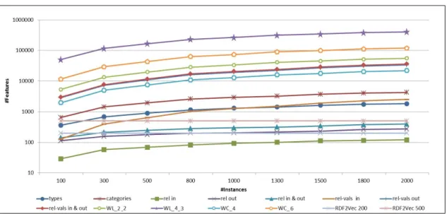
5.4. Features Increase Rate
Finally, we conduct a scalability experiment, where we examine how the number of instances affects the number of generated features by each feature
genera-tion strategy. For this purpose we use theMetacritic Moviesdataset. We start with a random sample of100 instances, and in each next step we add200(or 300) unused instances, until the complete dataset is used, i.e.,2,000instances. The number of generated features for each sub-sample of the dataset using each of the feature generation strategies is shown in Figure 3.
From the chart, we can observe that the number of generated features sharply increases when adding more samples in the datasets, especially for the strate-gies based on graph substructures.
In contrast, the number of features remains constant when using the RDF2Vec approach, as it is fixed to 200 or 500, respectively, independently of the number of samples in the data. Thus, by design, it scales to larger datasets without increasing the dimensionality of the dataset.
6. Entity and Document Modeling
Calculating entity relatedness and similarity are fun-damental problems in numerous tasks in information retrieval, natural language processing, and Web-based knowledge extraction. While similarity only considers subsumption relations to assess how two objects are alike, relatedness takes into account a broader range of relations, i.e., the notion of relatedness is wider than that of similarity. For example, “Facebook” and “Google” are both entities of the classcompany, and they have high similarity and relatedness score. On the other hand, “Facebook” and “Mark Zuckerberg” are not similar at all, but are highly related, while “Google” and “Mark Zuckerberg” are not similar at all, and have lower relatedness value compared to the first pair of entities.
6.1. Approach
In this section, we introduce several approaches for entity and document modeling based on the previously built latent feature vectors for entities.
6.1.1. Entity Similarity
mea-Fig. 3. Features increase rate per strategy (log scale).
sure, which is applied on the vectors of the entities. Formally, the similarity between two entities e1 and
e2, with vectorsV1andV2, is calculated as the cosine similarity between the vectorsV1andV2:
sim(e1, e2) =
V1·V2
||V1|| · ||V2|| (6)
6.1.2. Document Similarity
We use those entity similarity scores in the task of calculating semantic document similarity. We follow a similar approach as the one presented in [60], where two documents are considered to be similar if many entities of the one document are similar to at least one entity in the other document. More precisely, we try to identify the most similar pairs of entities in both docu-ments, ignoring the similarity of all other pairs.
Given two documentsd1 andd2, the similarity be-tween the documentssim(d1, d2)is calculated as fol-lows:
1. Extract the sets of entitiesE1andE2in the doc-umentsd1andd2.
2. Calculate the similarity score sim(e1i, e2j) for each pair of entities in documentd1andd2, where
e1i∈E1ande2j ∈E2
3. For each entity e1i ind1 identify the maximum similarity to an entity ind2max_sim(e1i, e2j ∈
E2), and vice versa.
4. Calculate the similarity score between the docu-mentsd1andd2as:
sim(d1, d2) = P|E1|
i=1max_sim(e1i,e2j∈E2)+P |E2|
j=1max_sim(e2j,e1i∈E1)
|E1|+|E2|
(7)
6.1.3. Entity Relatedness
In this approach we assume that two entities are re-lated if they often appear in the same context. For ex-ample, “Facebook” and “Mark Zuckerberg”, which are highly related, are often used in the same context in many sentences. To calculate the probability of two en-tities being in the same context, we make use of the RDF2Vec models and the set of sequences of entities generated as described in Section 3. Given a RDF2vec model and a set of sequences of entities, we calculate the relatedness between two entitiese1ande2, as the probabilityp(e1|e2)calculated using the softmax func-tion. In the case of a CBOW model, the probability is calculated as:
p(e1|e2) =
exp(vT e2v
0
e1)
PV
e=1exp(veT2v 0
e)
, (8)
wherev0
eis the output vector of the entitye, andV is the complete vocabulary of entities.
In the case of a skip-gram model, the probability is calculated as:
p(e1|e2) = exp(v
0T
e1ve2)
PV
e=1exp(ve0Tve2)
, (9)
6.2. Evaluation
For both tasks of determining entity relatedness and document similarity, we use existing benchmark datasets to compare the use of RDF2Vec models against state of the art approaches.
6.2.1. Entity Relatedness
For evaluating the entity relatedness approach, we use the KORE dataset [27]. The dataset consists of 21 main entities, whose relatedness to the other 20 entities each has been manually assessed, leading to 420 rated entity pairs. We use the Spearman’s rank correlation as an evaluation metric.
We use two approaches for calculating the related-ness rank between the entities, i.e. (i) the entity simi-larity approach described in section 6.1.1; (ii) the en-tity relatedness approach described in section 6.1.3.
We evaluate each of the RDF2Vec models sepa-rately. Furthermore, we also compare to the Wiki2vec model,16which is built on the complete Wikipedia cor-pus, and provides vectors for each DBpedia entity.
Table 6 shows the Spearman’s rank correlation re-sults when using the entity similarity approach. Table 7 shows the results for the relatedness approach. The results show that the DBpedia models outperform the Wikidata models. Increasing the number of walks per entity improves the results. Also, the skip-gram models outperform the CBOW models continuously. We can observe that the relatedness approach outperforms the similarity approach.
Furthermore, we compare our approaches to sev-eral state-of-the-art graph-based entity relatedness ap-proaches:
– baseline: computes entity relatedness as a func-tion of distance between the entities in the net-work, as described in [80].
– KORE: calculates keyphrase overlap relatedness, as described in the original KORE paper [27]. – CombIC: semantic similarity using a Graph Edit
Distance based measure [80].
– ER: Exclusivity-based relatedness [30].
The comparison, shown in Table 8, shows that our entity relatedness approach outperforms all the rest for each category of entities. Interestingly enough, the en-titysimilarityapproach, although addressing a differ-ent task, also outperforms the majority of state of the art approaches.
16https://github.com/idio/wiki2vec
6.3. Document Similarity
To evaluate the document similarity approach, we use the LP50 dataset [35], namely a collection of 50 news articles from the Australian Broadcasting Cor-poration (ABC), which were pairwise annotated with similarity rating on a Likert scale from 1 (very differ-ent) to 5 (very similar) by 8 to 12 different human an-notators. To obtain the final similarity judgments, the scores of all annotators are averaged. As a evaluation metrics we use Pearson’s linear correlation coefficient and Spearman’s rank correlation plus their harmonic mean.
Again, we first evaluate each of the RDF2Vec mod-els separately. Table 9 shows document similarity re-sults. As for the entity relatedness, the results show that the skip-gram models built on DBpedia with 8 hops lead to the best performances.
Furthermore, we compare our approach to several state-of-the-art graph-based document similarity ap-proaches:
– TF-IDF: Distributional baseline algorithm. – AnnOv: Similarity score based on annotation
overlap that corresponds to traversal entity simi-larity with radius 0, as described in [60].
– Explicit Semantic Analysis (ESA) [18].
– GED: semantic similarity using a Graph Edit Dis-tance based measure [80].
– Salient Semantic Analysis (SSA), Latent Seman-tic Analysis (LSA) [25].
– Graph-based Semantic Similarity (GBSS) [60].
The results for the related approaches were copied from the respective papers, except for ESA, which was copied from [60], where it is calculated via public ESA REST endpoint.17The results, shown in Table 10, show that our document similarity approach outper-forms all of the related approaches for both Pearson’s linear correlation coefficient and Spearman’s rank cor-relation, as well as their harmonic mean.
We do not compare our approach to the machine-learning approach proposed by Huang et al. [28], be-cause that approach is a supervised one, which is tai-lored towards the dataset, whereas ours (as well as the others we compare to) are unsupervised.
Table 6
Similarity-based relatedness Spearman’s rank correlation results
Model IT companies Hollywood
Celebrities
Television Series
Video Games
Chuck Norris
All 21 entities
DB2vec SG 200w 200v 4d 0.525 0.505 0.532 0.571 0.439 0.529
DB2vec CBOW 200w 200v 0.330 0.294 0.462 0.399 0.179 0.362
DB2vec CBOW 500w 200v 4d 0.538 0.560 0.572 0.596 0.500 0.564
DB2vec CBOW 500w 500v 4d 0.546 0.544 0.564 0.606 0.496 0.562
DB2vec SG 500w 200v 4d 0.508 0.546 0.497 0.634 0.570 0.547
DB2vec SG 500w 500v 4d 0.507 0.538 0.505 0.611 0.588 0.542
DB2vec CBOW 500w 200v 8d 0.611 0.495 0.315 0.443 0.365 0.461
DB2vec CBOW 500w 500v 8w 0.486 0.507 0.285 0.440 0.470 0.432
DB2vec SG 500w 200v 8w 0.739 0.723 0.526 0.659 0.625 0.660
DB2vec SG 500w 500v 8w 0.743 0.734 0.635 0.669 0.628 0.692
WD2vec CBOW 200w 200v 4d 0.246 0.418 0.156 0.374 0.409 0.304
WD2vec CBOW 200w 500v 4d 0.190 0.403 0.103 0.106 0.150 0.198
WD2vec SG 200w 200v 4d 0.502 0.604 0.405 0.578 0.279 0.510
WD2vec SG 200w 500v 4d 0.464 0.562 0.313 0.465 0.168 0.437
Wiki2vec 0.613 0.544 0.334 0.618 0.436 0.523
Table 7
Context-based relatedness Spearman’s rank correlation results
Model IT companies Hollywood
Celebrities
Television Series
Video Games
Chuck Norris
All 21 entities
DB2vec SG 200w 200v 4d 0.643 0.547 0.583 0.428 0.591 0.552
DB2vec CBOW 200w 200v 0.361 0.326 0.467 0.426 0.208 0.386
DB2vec CBOW 500w 200v 4d 0.671 0.566 0.591 0.434 0.609 0.568
DB2vec CBOW 500w 500v 4d 0.672 0.622 0.578 0.440 0.581 0.578
DB2vec SG 500w 200v 4d 0.666 0.449 0.611 0.360 0.630 0.526
DB2vec SG 500w 500v 4d 0.667 0.444 0.609 0.389 0.668 0.534
DB2vec CBOW 500w 200v 8d 0.579 0.484 0.368 0.460 0.412 0.470
DB2vec CBOW 500w 500v 8d 0.552 0.522 0.302 0.487 0.665 0.475
DB2vec SG 500w 200v 8d 0.811 0.778 0.711 0.658 0.670 0.736
DB2vec SG 500w 500v 8d 0.748 0.729 0.689 0.537 0.625 0.673
WD2vec CBOW 200w 200v 4d 0.287 0.241 -0.025 0.311 0.226 0.205
WD2vec CBOW 200w 500v 4d 0.166 0.215 0.233 0.335 0.344 0.243
WD2vec SG 200w 200v 4d 0.574 0.671 0.504 0.410 0.079 0.518
WD2vec SG 200w 500v 4d 0.661 0.639 0.537 0.395 0.474 0.554
Wiki2vec 0.291 0.296 0.406 0.353 0.175 0.329
7. Recommender Systems
As discussed in Section 2.3, theLinked Open Data
(LOD) initiative [5] has opened new interesting possi-bilities to realize better recommendation approaches. Given that the items to be recommended are linked to a LOD dataset, information from LOD can be ex-ploited to determine which items are considered to be similar to the ones that the user has consumed in the past, allowing to discover hidden information and
Table 8
Spearman’s rank correlation results comparison to related work
Approach IT
companies
Hollywood Celebrities
Television Series
Video Games
Chuck Norris
All 21 entities
baseline 0.559 0.639 0.529 0.451 0.458 0.541
KORE 0.759 0.715 0.599 0.760 0.498 0.698
CombIC 0.644 0.690 0.643 0.532 0.558 0.624
ER 0.727 0.643 0.633 0.519 0.477 0.630
DB_TransE -0.023 0.120 -0.084 0.353 -0.347 0.070
DB_TransH -0.134 0.185 -0.097 0.204 -0.044 0.035
DB_TransR -0.217 0.062 0.002 -0.126 0.166 0.058
DB2Vec Similarity 0.743 0.734 0.635 0.669 0.628 0.692
DB2Vec Relatedness 0.811 0.778 0.711 0.658 0.670 0.736
Table 9
Document similarity results - Pearson’s linear correlation coefficient (r) Spearman’s rank correlation (ρ) and their harmonic meanµ
Model r ρ µ
DB2vec SG 200w 200v 4d 0.608 0.448 0.516 DB2vec CBOW 200w 200v 4d 0.562 0.480 0.518 DB2vec CBOW 500w 200v 4d 0.681 0.535 0.599 DB2vec CBOW 500w 500v 4d 0.677 0.530 0.594 DB2vec SG 500w 200v 4d 0.639 0.520 0.573 DB2vec SG 500w 500v 4d 0.641 0.516 0.572 DB2vec CBOW 500w 200v 8d 0.658 0.491 0.562 DB2vec CBOW 500w 500v 8d 0.683 0.512 0.586 DB2vec SG 500w 200v 8d 0.708 0.556 0.623
DB2vec SG 500w 500v 8d 0.686 0.527 0.596 WD2vec CBOW 200w 200v 4d 0.568 0.383 0.458 WD2vec CBOW 200w 500v 4d 0.593 0.386 0.467 WD2vec SG 200w 200v 4d 0.606 0.385 0.471 WD2vec SG 200w 500v 4d 0.613 0.343 0.440
Wiki2vec 0.662 0.513 0.578
DB_TransE 0.565 0.432 0.490
DB_TransH 0.570 0.452 0.504
DB_TransR 0.578 0.461 0.513
Table 10
Comparison of the document similarity approach to the related work
Approach r ρ µ
TF-IDF 0.398 0.224 0.287 AnnOv 0.590 0.460 0.517
LSA 0.696 0.463 0.556
SSA 0.684 0.488 0.570
GED 0.630 \ \
ESA 0.656 0.510 0.574
GBSS 0.704 0.519 0.598
DB2Vec 0.708 0.556 0.623
RDF graph embeddings are a promising way to ap-proach those challenges and build content-based rec-ommender systems. As for entity similarity in the pre-vious section, the cosine similarity between the latent vectors representing the items can be interpreted as a measure of reciprocal proximity and then exploited to produce recommendations.
In this section, we explore the development of a hy-brid RS, leveraging the latent features extracted with RDF2Vec. The hybrid system takes advantage of both RDF graph embeddings and Factorization Machines (FMs) [66], an effective method combining Support Vector Machines with factorization models.
7.1. Factorization Machines
ˆ
y(x) =w0+ n
X
i=1
wixi+ n
X
i=1 n
X
j=i+1
(viTvj)xixj (10)
whereyˆrepresents the estimate of functiony. In (10) the parameters to be estimated are the global bias
w0 ∈ R, the vectorw = [w1, ..., wn] ∈ Rn whose componentwi models the strength of theithvariable and a matrixV ∈ Rn×k, which describes thei
th vari-able with itsith rowvi, i.e., with a vector of sizek, wherekis a hyperparameter defining the factorization dimensionality. On the other hand the model equation for a SVM of the same degree 2 is defined as:
ˆ
y(x) =w0+ √
2 n
X
i=1
wixi+ n
X
i=1
w(2)i,ix2i+
√ 2
n
X
i=1 n
X
j=i+1
wi,j(2)xixj (11)
with model parametersw0∈ R,w∈ Rnand the sym-metric matrixW(2)∈ Rn×n. From the comparison of equations (10) and (11) we can realize that both model all nested interactions up to degree 2 but with a fun-damental difference: the estimation of the interactions between variables in the SVM model is done directly and independently withwi,jwhereas it is parametrized in the FM model. In other words, parameterswi,jand
wi,lwill be completely independent in the SVM case while parametersvT
i vjandvTivloverlap thanks to the shared parametervi.
The strength of FMs models is also due to linear complexity [66] and due to the fact that they can be optimized in the primal and they do not rely on support vectors like SVMs. Finally, [66] shows that many of the most successful approaches for the task of collab-orative filtering are de facto subsumed by FMs, e.g., Matrix Factorization [84,78] and SVD++ [32].
7.2. Experiments
We evaluate different variants of our approach on three datasets, and compare them to common ap-proaches for creating content-based item representa-tions from LOD, as well as to state of the art collabo-rative and hybrid approaches. Furthermore, we inves-tigate the use of two different LOD datasets as back-ground knowledge, i.e., DBpedia and Wikidata.
7.2.1. Datasets
In order to test the effectiveness of vector space em-beddings for the recommendation task, we have per-formed an extensive evaluation in terms of ranking accuracy on three datasets belonging to different do-mains, i.e.,Movielens18for movies,LibraryThing19
for books, andLast.fm20for music. The first dataset,
Movielens 1M, contains 1 million 1-5 stars rat-ings from 6,040 users on 3,952 movies. The dataset
LibraryThingcontains more than 2 millions rat-ings from 7,279 users on 37,232 books. As there are many duplicated ratings in the dataset, which oc-cur when a user has rated the same item more than once, her last rating is selected. The unique ratings are 749,401, in the range from 1 to 10. BothMovielens
andLibraryThingdatasets contain explicit ratings, and to test the approach also on implicit feedbacks, a third dataset built on the top of theLast.fm mu-sic system is considered.Last.fm contains 92,834 interactions between 1,892 users and 17,632 musical artists. Each interaction is annotated with the corre-sponding listening count.
The original datasets are enriched with background information using the item mapping and linking to DBpedia technique described in [58], whose dump is available publicly.21 Since not all the items have a corresponding resource in DBpedia, after the map-ping, the versions of Movielens, LibraryThing and Last.fm datasets contain 3,883 movies, 11,695 books, and 11,180 musical artists, respectively.
The datasets are finally preprocessed to guarantee a fair comparison with the state of the art approaches described in [55]. Here, the authors propose to (i) re-move popularity biases from the evaluation not con-sidering the top 1% most popular items, (ii) reduce the sparsity ofMovielensdataset in order to have at least a sparser test dataset and (iii) remove from
LibraryThingandLast.fmusers with less than five ratings and items rated less than five times. The fi-nal statistics on the three datasets are reported in Table 11.
7.2.2. Evaluation Protocol
The ranking setting for the recommendation task consists of producing a ranked list of items to suggest to the user and in practical situations turns into the
so-18http://grouplens.org/datasets/movielens/ 19https://www.librarything.com/
20http://www.lastfm.com
21https://github.com/sisinflab/