Research Article
A Fast Algorithm for Solving a Class of the Linear
Complementarity Problem in a Finite Number of Steps
Yamna Achik,
1Asmaa Idmbarek,
1Hajar Nafia,
1Imane Agmour,
1and Youssef El foutayeni
1,21Analysis, Modeling and Simulation Laboratory, Hassan II University, Morocco 2Unit for Mathematical and Computer Modeling of Complex Systems, IRD, France Correspondence should be addressed to Youssef El foutayeni; [email protected]
Received 26 August 2020; Accepted 18 December 2020; Published 30 December 2020
Academic Editor: Victor Kovtunenko
Copyright © 2020 Yamna Achik et al. This is an open access article distributed under the Creative Commons Attribution License, which permits unrestricted use, distribution, and reproduction in any medium, provided the original work is properly cited. The linear complementarity problem is receiving a lot of attention and has been studied extensively. Recently, El foutayeni et al. have contributed many works that aim to solve this mysterious problem. However, many results exist and give good approximations of the linear complementarity problem solutions. The major drawback of many existing methods resides in the fact that, for large systems, they require a large number of operations during each iteration; also, they consume large amounts of memory and computation time. This is the reason which drives us to create an algorithm with afinite number of steps to solve this kind of problem with a reduced number of iterations compared to existing methods. In addition, we consider a new class of matrices called the E-matrix.
1. Introduction
In the last decades, the complementarity problem has played a very important role in several domains. It has been the focus of many researchers and scientists. As an example, we can cite the works of Cottle [1, 2] published between 1964 and 1966. Note that the above problem appears in older works without reporting the name of complementarity prob-lems. In particular, we mention the work of Du Val [3] and Ingleton [4]. Letf be a function defined inℝntoℝn. A com-plementarity problem (CP) associated with the function f consists tofind a vector z∈ℝn such as z≥0,fðzÞ≥0, and
zTfðzÞ= 0. If the functionf is affine, it is presented in form fðzÞ=Mz+q,whereqis a vector ofℝn andM is a square matrix of ordern. Then, we have a linear complementarity problem denoted by LCPðM,qÞ. The origin of the name complementarity comes from the fact that ifz∈ℝn
+is a
solu-tion of a linear complementarity problem, then zi= 0 or
fiðzÞ= 0 for all i= 1, 2,⋯,n. The linear complementarity problem has been widely studied by researchers from a
variety of backgrounds, which has been a rich and varied literature (see [5–17] and references therein). In [18], Kadiri and Yassine described a new purification method for solving monotonic linear complementarity problems. In their paper, the proposed method is associated with each iterate of the sequence, generated by an interior point method, one basis that is not necessarily feasible. The authors proved that, under the strict complementarity and nondegeneracy hypotheses, the sequence of bases converges on a definite number of iter-ations to an optimal basis which gives the exact solution to the problem. In [19], to solve the linear complementarity problem, Alves and Judice [19] proposed a pivoting heuristic based on tabu search and its integration into an enumerative framework. Recently, El foutayeni et al. [20–28] added a contribution to the resolution of the linear complementarity problem. In particular, in [27], they proved the equivalent between solving a linear complementarity problem and solv-ing a nonlinear equation. Also, they give a globally convergent hybrid algorithm which is based on vector divisions for solving the linear complementarity problem. In [27], the same authors Volume 2020, Article ID 8881915, 8 pages
determined the conditions that allow a linear complementar-ity problem to have a solution. They calculated the solution when it exists. In [24], they proposed to solve the linear complementarity problem in the case where it has several solutions. The aim of [29] is to propose an iterative method of interior points that converge in the polynomial time to the best solution of the linear complementarity problem; this convergence requires at mostoðn0,5LÞiterations, where
n is the number of the variables and L is the length of a binary coding of the input; furthermore, the algorithm does not exceed oðn3,5LÞ arithmetic operations until its
conver-gence. In [24], El foutayeni and Khaladi have shown that the linear complementarity problemLCPðM,qÞis completely equivalent tofinding thefixed point of the mapx= maxð0,
ðI−MÞx−qÞ, and they showed that tofind an approxima-tion of the soluapproxima-tion to the second problem, they proposed an algorithm that starts from an arbitrary interval vector Xð0Þ, then they generalize a sequence of the interval vector
ðXðkÞÞk=1,⋯that converges to the best solution of linear com-plementarity problems. Newly, in [30], for solving the linear complementarity problem, Wang et al. [31] propose an inte-rior point method tofind the solution of the linear comple-mentarity problem, where the matrix is a real square hidden Z-matrix. In this context, we can see the works [31–39].
It is well known that it is impossible to ensure the exis-tence of a linear complementarity problem solution associ-ated with any matrix and vector. This leads us to ask the following questions: Under which conditions on the matrix and the vector does this type of problem admit a solution, and if it exists, what are the conditions for the uniqueness of this solution? Once the existence and uniqueness are assured, how we can express this solution according to the data of the problem? Despite the great importance of the lin-ear complementarity problems in several areas, they are not yet completely resolved. However, many results exist and give good approximations of the solutions, but the main dis-advantage of many existing methods resides in the fact that, for large systems, they require a large number of operations during each iteration and they consume large amounts of memory and computation time. This is the reason that drives us to look for new methods that deal with this kind of prob-lem which lower the number of operations at each iteration compared to existing methods.
In the present work, we formulate an algorithm that can solve the linear complementarity problemLCPðM,qÞ. This algorithm has afinite number of steps and converges to the solution. Also, we consider a new class of matrices called theE-matrix. The algorithm has been surprisingly effective. A numerical implementation of the algorithm is given in this work.
We organized this document as follows. In Section 1, we give preliminary definitions and we list some initial notations that we need throughout this document. In Section 2, we present the proposed linear complementarity problem under some conditions. In Section 3, we formulate an algorithm for solving our linear complementarity problem with the E class’s matrix. And in Section 4, we give numerical examples to confirm the theoretical part of our algorithm.
2. Preliminary and Notations
In this section, we recall preliminary definitions and general notations used in this paper.
For any positive integern, let ℝn×n be the ensemble of all real n×nmatrices. We denote by I the matrix of iden-tity, ek is thekthcolumn of I, ande=ð1,⋯, 1ÞT is a vector where all entries equal to 1. We also use the following notation Ck· and C·k to represent the kth row and the kth column of the C matrix, respectively; Yn=fy/∣y∣=eg is the ensemble of all ±1 vectors of ℝn, and its cardinality is equal to 2n. For each x∈Rn, we define his sign vector
sgnðxÞ by ðsgnðxÞÞi= 1 if xi≥0 and ðsgnðxÞÞi=−1 if xi < 0 with i∈f1, 2,⋯,ng. Then, sgnðxÞ∈Yn. For each z∈ ℝn, we denote T
z= diagðz1,⋯,znÞ.
Definition 1. GivenM∈ℝn×n, the set of matrices
A=fS∈ℝn×n:jS−ðM+IÞj≤I+j jMg=½M−j jM, 2I+M+j jM,
ð1Þ
is called an interval matrix.
Definition 2. A square interval matrixAis called regular if eachS∈Ais regular and singular if it existsS∈Asingular.
Proposition 3.An interval matrixAis singular if and only if the inequality
M+I
ð Þx
j j≤ðI+j jMÞj jx, ð2Þ
has a nontrivial solution.
Proof.We suppose thatAcontains a singular matrixS, then there exist x≠0such thatSx= 0, which implies thatjðM+
IÞxj=jðM+IÞx−Sxj≤ðI+jMjÞjxj:Conversely, let (2) hold for x≠0: Define y∈ℝn and z∈Y
n by yi=½ðI+MÞxi/
½ðI+∣M∣Þ∣x∣i, for i=f1,⋯,ng. If ½ðI+∣M∣Þ∣x∣i> 0 or
yi= 1and ½ðI+∣M∣Þ∣x∣i= 0taking into account that z= sgnðxÞ, then Tzx=jxj: Hence, ½ððI+MÞ−TyðI+∣M∣ÞTzÞ
xi=ððI+MÞxÞi−yiððI+∣M∣Þ∣x∣Þi= 0for eachi.
Therefore,ðI+MÞ−TyðI+∣M∣ÞTzis singular, and since
jyij≤1for each i due to ð1Þ, it follows that jðI+MÞ−Ty
ðI+jMjÞTz−ðI+MÞj=jTyðI+jMjÞTzj≤ðI+∣M∣Þ: Hence,ðI+MÞ−TyðI+∣M∣ÞTz∈AandAis singular. We use the previous proposition to show the regularity or the singularity of the matrixAin some cases.
Proposition 4.LetAbe regular and let
I+M+ðI−MÞTz′
ð Þx′=ðI+M+ðI−MÞTz″Þx″, ð3Þ
hold for somez′,z″∈Ynandx′≠x″:
Proof.We assume that for eachi,zi′zi′′=−1impliesxi′xi′′≤0,so ∣xi′−xi′′∣=∣xi′∣+∣xi′′∣. We shall prove in this case that
Tz′x′−Tz″x″
≤x′−x″, ð4Þ
i.e., the inequalityjzi′xi′−zi′′x′′ij≤ ∣xi′−xi′′∣ holds for eachi: Since jzi′xi′−zi′′xi′′j=jzi′ðxi′−zi′zi′′xi′′Þj=jxi′−zi′zi′′xi′′j, this is clear fact forzi′zi′′=−1:Ifzi′zi′′=−1,sojzi′xi′−zi′′xi′′j=jxi′+xi′′j≤ ∣
xi′∣+∣xi′′∣=∣xi′−xi′′∣which together proves (3).
Now, from (3), we have jðI+MÞðx′−x″Þj=jðI−MÞ
ðTz′x′−Tz″x″Þj≤ðI+jMjÞjx′−x″j, by (4), with x′−x″ ≠0, thenAis singular following the first proposition, and this is a contradiction.
We use the Sherman-Morrison formula to prove the effi -ciency of the proposed algorithm.
LetA∈ℝn×nbe nonsingular matrix,ðb,cÞ∈ℝn×n, and let α= 1 +cTA−1b.
So, we havedetðA+bcTÞ=αdetðAÞ,ifα= 0,thenA+
bcT is singular, and if α≠0, we deduce that ðA+bcTÞ−1=
A−1−ð1/αÞA−1bcTA−1(see [40]).
3. Main Results
It is a known fact (see El foutayeni and Khaladi [27]) that the linear complementarity problem LCPðq,MÞ is completely equivalent to solving the equation ðI+MÞx+
ðI−MÞ∣x∣ =q, wherez=∣x∣ −xand w=∣x∣+x. To pres-ent the algorithm, we define a new class of matrices that we call the class of E-matrices.
Definition 5. Let M∈ℝn×n . The matrix M is called the
E -matrix if all the principal minors ofMare nonzero and if all the eigenvalues ofMare different from−1.
Notation 6. We denoteEthe set ofE-matrices
E=fM∈Mn/MP≠0 andλi≠ −1,∀i∈f1, 2,⋯,ngg, ð5Þ such thatMPis the set of the principal minors ofMandλiis the eigenvalues ofM.
Lemma 7.We have the equivalence between the following four properties of a matrixA:
(1) All the principal minors of matrixAare positive (2) For each vectorx≠0,there existsisuch thatxiyi>0,
withy=Ax
(3) For each vectorx≠0, there exists a diagonal matrix
Dx≥0such thatðAx,DxxÞ>0
(4) The real eigenvalues associated withAand every prin-cipal minor ofAare positive
Proof.1⇒2:We denote byNthe set of indices1, 2, 3⋯,n: We select an arbitrary vectorx≠0,and we assume thatxiyi
≤0, for each i∈N, withy=Ax. LetΓ=fi/xi≠0g:Clearly Γ≠0:IfAðΓÞis the main submatrix with rows and columns ofΓ,xðΓÞis the vector wherein coordinates have indices ofΓ and coincide with those ofx; hence, fori∈Γ, the coordinates ziof the vectorz=AðΓÞxðΓÞcoincide withyi:So, there exists a diagonal matrixU≥0(overΓ×Γ) such asz=−UxðΓÞ,i.e.,
ðAðΓÞ+UÞxðΓÞ= 0. Therefore, the matrix AðΓÞ+U is singular. Note that the principal minors ofAðΓÞare positive. So, we have the same result forAðΓÞ+U sinceU is diagonal positive. This is a contradiction that proves the implication.
2⇒3. We suppose thatx≠0is a vector,y=Ax, andiis the index for whichxiyi> 0:There exists a positive numberη, such as xiyi+η∑j≠ixjyjis positive. To prove this, it is suffi -cient to chooseDxas the diagonal matrix, wheredii= 1and
djj=η,forj≠i:3⇒4. Let0≠Γ⊂Nand letλbe a real eigen-value ofAðΓÞwith the eigenvectorxðΓÞ:We denote byxthe vector with the coordinates xi that coincide with those of
xðΓÞfor i∈Γ: In accordance with (4), there exists a diag-onal matrix Dx≥0 such that ðAx,DxxÞ> 0: But evidently,
ðAx,DxxÞ=λðx,DxxÞ, since ðx,DxxÞ> 0. Then, we have λ > 0:4⇒1. Now, using the fact that the determinant of a matrix A is equal to the product of all eigenvalues of A and that the product of the nonreal eigenvalues of a real matrix is positive, we can easily complete the proof.
Lemma 8.Any matrixP-matrix is anE-matrix.
Proof.LetMbe aP-matrix. Then, all principal minors ofM are positive. From the previous Lemma, we can deduce that all real eigenvalues ofMare positive sinceMis anE-matrix.
It is easy to check that the identity matrix is anE-matrix; every symmetric positive definite matrix is anE-matrix and any Hilbert matrix is an E-matrix (we recall that a Hilbert matrix is a square matrix of general termshij= 1/ði+j−1Þ).
Theorem 9.For all matrixM∈E‐matricesand vectorq∈ℝn, the following algorithm “SolveLCP” has a finite number of steps and converges to the solution of the linear complemen-tarity problemLCPðM,qÞif it exists.
The linear complementarity problemLCPðM,qÞimplies I+M
ð Þx+ðI−MÞj jx =q: ð6Þ
According to a change of variables,z=∣x∣ −x and w= ∣x∣+x. Hence, if we considerTz= diagðzÞwithz= sgnðxÞ, then the equation (4) becomes
I+M
ð Þ+ðI−MÞTz
ð Þx=q: ð7Þ
The problem is that we do not know the values of eitherx or z, but we know that they must satisfyTzx=jxj≥0, i.e.,
zixi≥0for eachi:
Step 1. The algorithm beginning with the vector p= 0and during each pass of the loop“while”it increases by 1; hence pk becomespk+ 1 which means that after a finite number
of steps,pk will become superior to2n−kand the algorithm will end.
Step 2.The initial point isz= sgnððI+MÞ−1qÞ; it is achiev-able sinceðI+MÞis a regular matrix; indeed, we haveM∈ E‐matrices, so all the principal minors of M are nonzero, and for allλeigenvalues ofM,λ≠ −1:Then, there existsv
∈ℝn such that Mv=λv: Therefore, ðI+MÞv=ð1 +λÞv; hence,ð1 +λÞis an eigenvalue ofðI+MÞ:
Step 3.x=ððI+MÞ+ðI−MÞTzÞ−
1
qis also feasible, since the matrixH=ððI+MÞ+ðI−MÞTzÞis regular. We have H=
ðHijÞ1≤i,j≤nwhere
Hij=
1 +mii
ð Þ+zið1−miiÞ, ifi=j,
mij−mijzj, ifi≠j: (
ð8Þ
Consequently,ðHÞij= 2ejifzj> 0orðHÞij= 2mijifzj< 0;
Mis regular becauseM∈E‐matrices. Therefore, all the col-umn vectors ofMare linearly independent, soHis regular. Step 4.Whenxandzare held, we calculatexz; we have two cases
Case 1.xizi> 0,for alli∈f1,⋯,ng,thenTzx≥0implies that
Tzx=∣x∣ and such x=ððI+MÞ+ðI−MÞTzÞ−
1
q, we find
ðI+MÞx+ðI−MÞ∣x∣ =ððI+MÞ+ðI−MÞTzÞx=q. So, x solves the equation (4) and z=∣x∣ −x is the solution of the linear complementarity problem LCPðM,qÞ.
Case 2. xizi< 0, we assume the existence of j such as j= minfi:xizi< 0gand we updated the matrix Tz and z. So, we bring backzjto−zj, and theTzmatrix will be modified. Then, for all realt,T~z=Tz−2tzjejeTj.
The matrix H will change to the matrix H~ defined by ~
H=H−2tzjðI−MÞejeTj.
Now checking the regularity of the matrixH~. We have, according to the formula of Sherman-Morrison, detðH~Þ=
ð1−2tzjeTjH−1ðI−MÞejÞdetðHÞ:
We consider C=−H−1ðI−MÞ, thendetðH~Þ=ð1 + 2tz
j
CjjÞdetðHÞ. Therefore, we have two possible cases
(a) If 1 + 2zjCjj≤0, we have Cjj≠0 and the function φ :ℝ⟶ℝdefined by φðtÞ= 1 + 2tzjCjj satisfies φð0Þφð1Þ= 1 + 2zjCjj≤0: Then, according to the Theorem of Intermediate Values, there existt0∈½0,
An algorithm for solving the linear complementarity problemLCPðM,qÞ function ½z∗= SolveLCPðM,qÞ
p= 0∈ℝn
z= sgnððI+MÞ−1qÞ x=ððI+MÞ+ðI−MÞTzÞ−1q
C=−ððI+MÞ+ðI−MÞTzÞ−1ðI−MÞ
whilezixi< 0for somei
j= minfi/zixi< 0g
if1 + 2zjCjj≤0
x=½;
display(no solution) return
end pj=pj+ 1
if log2ðpjÞ>n−j x=½;
display(no solution) return
end
if1 + 2zjCjj> 0
Tz=Tz−2zjejeTj ;
zj=−zj;
α=ðð2zjÞ/ðð1−2zjCjjÞÞÞ;
x=x+αxjC·j;
C=C+αC·jCj·;
end end z∗=∣x∣ −x;
end
1 such as φðt0Þ= 0, so t0=−1/2zjjCjj and thus detðH−2t0zjðI−MÞejeTjÞ= 0; hence, in this case, the matrixH~is singular and the solution does not exist (b) If1 + 2zjCjj> 0, we have the matrix ðI+MÞ+ðI−
MÞTz=H−2zjðI−MÞejeTj which is regular fort= 1,then according to Sherman-Morrison’s formula
I+M
ð Þ+ðI−MÞTz
½ −1
=H−1+H −12
zjðI−MÞejeTjH−1 1 + 2zjCjj =H−1+αC·jeTjH−1:
ð9Þ
We obtain α= −2zj
1 + 2zjCjj ,
x=H−1q+αC·jeTjH−
1
q=x+αxjC·j,
C=−H−1ðI−MÞ−αC·jeTjH−1ðI−MÞ=C+αCj·C·j: 8 > > > > > < > > > > > :
ð10Þ
Therefore, we conclude that the matrix C plays an important role for giving an explicit calculation of x=
ððI+MÞ+ðI−MÞTzÞ−
1
q at each step.
Step 5.Let us show that iflog2pj>n−j, then the matrixAis singular and the solutionxdoes not exist. This will be proven by showing that ifAis regular sopj≤2n−jfor eachj. So, we can demonstrate that every jcan appear at most2n−jtimes
ðj=n,⋯, 1Þ; we have two cases
Case 1.j=n: we suppose thatnappears at least twice in the sequence and that x′,z′ and x},z} correspond to the two closest occurrences, that is to say, that there is no other occurrence of n between them. So, xi′zi′≥0 and xizi≥0
fori=f1,⋯,n−1g,andxn′z′n< 0,x}nz}n< 0,zn′zn}=−1, which implies that xn′zn′xn}z}n> 0 and xn′xn}< 0: Then, xi′zi′xizi≥0
for all i=f1,⋯,n−1g. But since I+M
ð Þ+ðI−MÞTz
½ x′=q=½ðI+MÞ+ðI−MÞTzx},
ð11Þ
we obtain the relation (11) using the fact that x=
½ðI+MÞ+ðI−MÞTz−
1
qand x′≠x} since xn′xn}< 0; it fol-lows from Proposition 4 that there is ani wherezi′zi}=−1 and xi′xi}> 0, which implies that x′izi′xi}zi}< 0, which is a contradiction, so n occurs at most once in the sequence. Case 2. j<n: letz′,x′ andz},x} correspond to two occur-rences of j, so that zi′xi′≥0,zixi≥0 for i=f1,⋯,j−1g,
zj′x′j< 0,zj}xj}< 0and zj′zj}=−1:This gives thatxi′zi′xizi≥0
for i=f1,⋯,j−1g,x′jz′jx}jz}j> 0 and x′jxj}< 0. Then, as the condition (11) holds because ofx=½ðI+MÞ+ðI−MÞTz−
1
q and x′≠x} since xn′xn}< 0, then Proposition 4 implies the existence of an iwhere zi′zi}=−1 and xi′xi}> 0, as well as xi′zi′xi}zi}< 0 so that i>j. So aszi′zi}=−1,i should have entered the sequence of j; there is an occurrence of some i>j in the sequence; this means, by the assumptions, that j cannot appear there more than ð2n−j−1+⋯+2 + 1Þ+ 1 = 2n−j times.
4. Numerical Examples
In this section, we demonstrate the effectiveness of our pro-posed algorithm in relation to the execution time and the number of iterations. To do this, we made comparisons between our algorithm and other existing methods. In the first, we give a simple example of a matrixE-matrix of order 4, for which wefind the solution in a short time. In the sec-ond example, we compare the results obtained by our method with those obtained by the method of El foutayeni et al., the method of Yu, and the method of Chen-Harker-Kanzow-Smale (CHKS), and in the third example, we com-pare the execution time of our method with the method of Lemke and the method of the interior point.
Example 10. Considering the next linear complementarity problem, where we search to determine a vectorzinℝ4such
thatz≥0,w=Mz+q≥0andzTw= 0, with
M=
4 2 0 3
−1 4 −3 −6
1 −1 1 1
0 1 0 5
2 6 6 6 6 6 4 3 7 7 7 7 7 5,q=
−1 2 −1 −1 2 6 6 6 6 6 4 3 7 7 7 7 7 5:
ð12Þ
It is easy to prove that the associated matrix M is anE-matrix, by applying the proposed algorithm. Then, we obtain z=ð0, 1, 2, 0ÞT and the elapsed time is 0.000547 seconds.
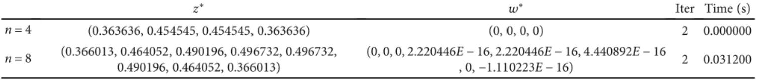
Example 11. In this example, we compare the results obtained with our method to those obtained with the method of El foutayeni, the method given by Yu, and the method of Chen-Harker-Kanzow-Smale (CHKS). For attending this, we adopt our MATLAB program to calcu-late the optimal solution z, the final values w=Mz+q, the number of iterations, and the time in seconds. Consider-ing the followConsider-ing linear complementarity problemLCPðM,
qÞ, where M=ðmijÞ1≤i,j≤n such as mii= 4 for i=j,mi,i+1=
mi+1,i=−1 for all i= 1,⋯,n, and it equals to 0 otherwise, andq=ðqiÞ1≤i≤nsuch asqi=−1:
Tables 1–4 present the summaries of the results obtained, where Iter represents the iteration numbers when the algo-rithm ends and Time indicates the total cost in seconds to resolve the problem.
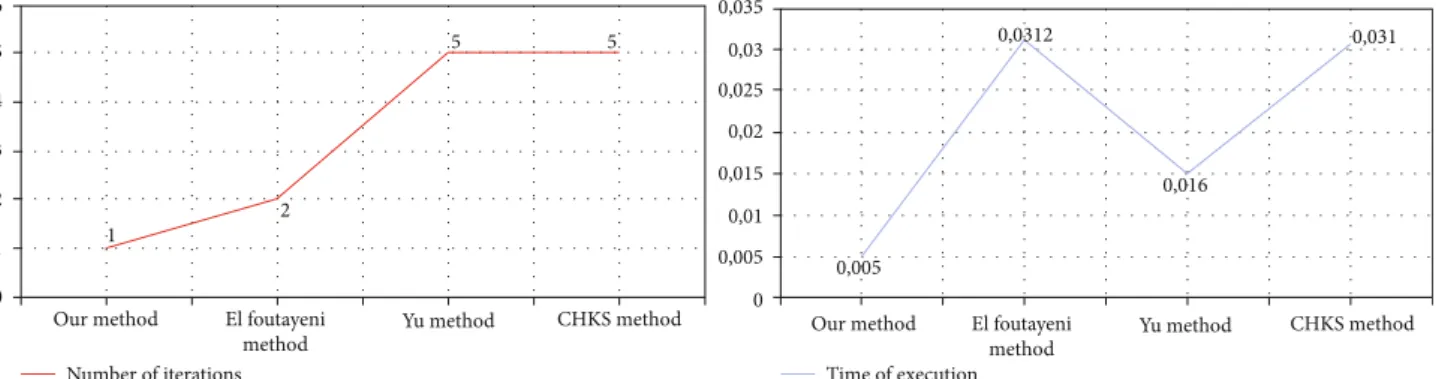
From Figures 1 and 2, we can notice that our method can be comparable with the method of El foutayeni, the method of Yu, and the method of CHKS, from the iteration numbers and CPU computation time in seconds.
Example 12. In this example, we compare three different methods in order to solve a linear complementarity problem
CPðM,qÞ. Thefirst one is our method, the second one is Lemke’s method, and the last one is the interior point method[30]. We take the same example, whereM=ðmijÞ1≤i,j≤nsuch asmii= 4,
mi,i+1=mi+1,i=−1for alli= 1,⋯,nand zero in the rest and
q=ðqiÞ1≤i≤nsuch asqi=−1:The matrixMis definitely positive, so we ensure the convergence of Lemke’s method. InTable 5, the first column represents the dimension of the linear complemen-tarity problem. The second provides (the third and the fourth) the computation time in seconds for Lemke’s method to be per-formed (interior point algorithm and our algorithm).
Based on this table, in the case wheren= 1000, we con-clude that Lemke’s method is divergently compared to time (it needs 334 seconds to display the results), but our Table1: Numeric outcomes of our method.
z∗ w∗ Iter Time (s)
n= 4 (0.3636, 0.4545, 0.4545, 0.3636) (0, 0, 0, 0) 1 0.0040
n= 8 (0.3660, 0.4641, 0.4902, 0.4967, 0.4967, 0.4902, 0.4641, 0.3660) (0, 0, 0, 0 0, 0, 0, 0) 1 0.0050 Table2: Numeric outcomes of the El foutayeni method.
z∗ w∗ Iter Time (s)
n= 4 (0.363636, 0.454545, 0.454545, 0.363636) (0, 0, 0, 0) 2 0.000000
n= 8 (0.366013, 0.464052, 0.490196, 0.496732, 0.496732,
0.490196, 0.464052, 0.366013)
(0, 0, 0, 2.220446E−16, 2.220446E−16, 4.440892E−16
, 0,−1.110223E−16) 2 0.031200
Table3: Numeric outcomes of the Yu method.
z∗ w∗ Iter Time
(s) n= 4 (0.363636, 0.454545, 0.454545, 0.363636) (0, 0,−1.11022E−16, 0) 5 0.031 n= 8 (0.366013, 0.464052, 0.490196, 0.496732, 0.496732, 0.490196, 0.464052,
0.366013)
(−1.11022E−16, 0, 0, 0, 0,−1.11022E−16,
0, 0) 5 0.016
Table4: Numeric outcomes of the CHKS method.
z∗ w∗ Iter Time
(s) n= 4 (0.363636, 0.454545, 0.454545, 0.363636) (−6.72751E−12,−5.38214E−12,−5.38214E−12,−6.72751E−12) 5 0.016 n= 8 (0.366013, 0.464052, 0.490196, 0.496732,
0.496732, 0.490196, 0.464052, 0.366013)
(−6.68399E−12,−5.27156E−12,−4.9909E−12,−4.92495E−12,
−4.92495E−12,−4.9909E−12,−5.27178E−12,−6.68399E−12) 5 0.031
Number of iterations
6 0,035
0,03 0,025 0,02
0,004
0
0,031
0,016 0,015
0,01 0,005 0 5
4 3 2 1 0
Our method El foutayeni method
Yu method CHKS method Our method El foutayeni
method Yu method
CHKS method Time of execution
1
2
5 5
Figure1: Comparison between our method with the method of El foutayeni, the method of Yu, and the method of CHKS as a function of time and number of iterations in the case wheren= 4.
method only needs 0.928443 seconds to find the solution ofLCPðM,qÞ. The same is said for the point interior method. We noticed that our algorithm is faster than the other algo-rithms compared to the execution time. Then, we can deduce that the performance of our method is effective.
5. Conclusion
Solving a linear LCP complementarity problem has been the goal of much research. Thus, in this article, we have proposed an algorithm allowing us to solve the LCP linear complemen-tarity problem. This algorithm has afinite number of steps and converges to the solution. In addition, we have consid-ered a new class of matrices called theE-matrix such that the algorithm is efficient. In perspective, we seek tofind a simple method to solve linear complementarity problems with any matrixM and vectorqwithout treating the cases on the matrixM, so that it is fast in execution time and in the number of iterations. A digital implementation of the algorithm is given in this work.
Data Availability
No data were used to support this study.
Conflicts of Interest
The authors declare that they have no conflicts of interest.
References
[1] R. W. Cottle,“Note on a fundamental theorem in quadratic programming,” Journal of the Society for Industrial and Applied Mathematics, vol. 12, no. 3, pp. 663–665, 1964. [2] R. W. Cottle,“Nonlinear programs with positively bounded
Jacobians,” SIAM Journal on Applied Mathematics, vol. 14, no. 1, pp. 147–158, 1966.
[3] P. Du Val,“The unloading problem for plane curves,”American Journal of Mathematics, vol. 62, no. 1/4, pp. 307–311, 1940. [4] A. W. Ingleton,“A problem in linear inequalities,”Proceedings
of the London Mathematical Society, vol. 16, pp. 519–536, 1966. [5] C. E. Lemke,“Bi-matrix equilibrium points and mathematical programming,”Management Science, vol. 11, no. 7, pp. 681– 689, 1965.
[6] R. W. Cottle,“The principal pivoting method of quadratic pro-gramming,”inMathematics of Decision Sciences, Part 1, G. B. Dantzig and A. F. Veinott, Eds., pp. 142–162, AMS, Provi-dence, RI, 1968.
[7] B. C. Eaves and C. E. Lemke,“Equivalence of LCP and PLS,” Mathematics of Operations Research, vol. 6, no. 4, pp. 475– 484, 1981.
[8] L. Mathiesen,“An algorithm based on a sequence of linear complementarity problems applied to a Walrasion equilibrium model: an example,” Mathematical Programming, vol. 37, no. 1, pp. 1–18, 1987.
[9] S. J. Chung,“NP-completeness of the linear complementarity problem,”Journal of Optimization Theory and Applications, vol. 60, no. 3, pp. 393–399, 1989.
[10] R. W. Cottle, J. S. Pang, and R. E. Stone,The Linear Comple-mentarity Problem, Academic Press, 1992.
[11] J. S. Pang and A. Gabriel,“NE/SQP: a robust algorithm for the nonlinear complementarity problem,” Mathematical Pro-gramming, vol. 60, no. 1-3, pp. 295–337, 1993.
[12] B. Chen and P. T. Harker,“A non-interior-point continuation method for linear complementarity problems,”SIAM Journal on Matrix Analysis and Applications, vol. 14, no. 4, pp. 1168– 1190, 1993.
[13] C. Geiger and C. Kanzow,“On the resolution of monotone complementarity problems,” Computational Optimization and Applications, vol. 5, no. 2, pp. 155–173, 1996.
[14] C. Kanzow,“Some non-interior continuation methods for lin-ear complementarity problems,” SIAM Journal on Matrix Analysis and Applications, vol. 17, no. 4, pp. 851–868, 1996. Number of iterations
6 0,035
0,03 0,025 0,02 0,015 0,01 0,005 0 5
4 3 2 1 0
Our method El foutayeni method
Yu method CHKS method Our method El foutayeni method
Yu method CHKS method Time of execution
1
2
0,005
0,0312
0,016
0,031 5 5
Figure2: Comparison between our method with the method of El foutayeni, the method of Yu, and the method of CHKS as a function of time and number of iterations in the case wheren= 8.
Table5: The execution time for the different methods. n Lemke Interior point Proposed algorithm
10 5 23 0.00447
20 8 34 0.005160
50 14 56 0.014906
100 32 148 0.030162
200 74 289 0.04148
400 126 518 0.110811
500 159 665 0.177190
[15] K. G. Murty,Linear Complementarity, Linear and Nonlinear Programming, Internet ed., 1997.
[16] R. W. Cottle and G. B. Dantzig,“George B. Dantzig: A legend-ary life in mathematical programming,” Mathematical Pro-gramming, vol. 105, no. 1, pp. 1–8, 2006.
[17] Z. Yu and Y. Qin,“A cosh-based smoothing Newton method for P0 nonlinear complementarity problem,”Nonlinear Anal-ysis: Real World Applications, vol. 12, no. 2, pp. 875–884, 2011. [18] A. Kadiri and A. Yassine,“Une procédure de purification pour les problèmes de complémentarité linéaire monotones,” RAIRO Operation Research, vol. 38, no. 1, pp. 63–83, 2004. [19] M. J. Alves and J. Judice,“On the use of a tabu pivoting
tech-nique for solving the linear complementarity problem,” AMO - Advanced Modeling and Optimization, vol. 13, pp. 111–140, 2011.
[20] Y. El Foutayeni, H. El Bouanani, and M. Khaladi,“An (m+1)-step iterative method of convergence order (m+2) for linear complementarity problems,”Journal of Applied Mathematics and Computing, vol. 54, pp. 229–242, 2017.
[21] Y. El Foutayeni and M. Khaladi,“The linear complementarity problem and a modified Newton’s method tofind its solution,” Bulletin of Mathematical Sciences and Applications, vol. 15, pp. 17–35, 2016.
[22] H. El Bouanani, Y. El Foutayeni, and M. Khaladi, “A new method for solving non-linear complementarity problems,” International Journal of Nonlinear Science, vol. 19, pp. 81–90, 2015.
[23] Y. El Foutayeni, H. El Bouanani, and M. Khaladi,“The linear complementarity problem and a method tofind all its solu-tions,” Information in Sciences and Computing, vol. 3, pp. 11–15, 2014.
[24] Y. El Foutayeni and M. Khaladi,“A min-max algorithm for solving the linear complementarity problem,” Journal of Mathematical Sciences, vol. 1, pp. 6–11, 2013.
[25] H. Jiang and L. Qi,“A new nonsmooth equations approach to nonlinear complementarity problems,”SIAM Journal on Con-trol and Optimization, vol. 35, no. 1, pp. 178–193, 1997. [26] Y. El Foutayeni and M. Khaladi,“General characterization of a
linear complementarity problem,”American Journal of Model-ing and Optimization, vol. 1, pp. 1–5, 2013.
[27] Y. Elfoutayeni and M. Khaladi,“Using vector divisions in solv-ing the linear complementarity problem,”Journal of Computa-tional and Applied Mathematics, vol. 236, no. 7, pp. 1919– 1925, 2012.
[28] Y. El Foutayeni and M. Khaladi,“A new interior point method for linear complementarity problem,”Applied Mathematical Sciences, vol. 4, pp. 3289–3306, 2010.
[29] R. Jana, A. K. Das, and A. Dutta,“On hidden Z-matrix and interior point algorithm,”Opsearch, vol. 56, no. 4, pp. 1108– 1116, 2019.
[30] A. Yassine,“Comparative study between Lemke’s method and the interior point method for the monotone linear comple-mentary problem,”Studia Universitatis Babes-Bolyai Mathe-matica, vol. 53, no. 3, pp. 119–132, 2008.
[31] W. Wang, Z. Zhou, S. A. Edalatpanah, and S. E. Najafi,“A new approach for the modulus-based matrix splitting algorithms,” IEEE Access, vol. 7, pp. 100143–100146, 2019.
[32] X. Wu and R. Ke,“Backward errors of the linear complemen-tarity problem,” Numerical Algorithms, vol. 83, no. 3, pp. 1249–1257, 2020.
[33] Z. Sun and X. Yang,“A generalized Newton method for a class of discrete-time linear complementarity systems,” European Journal of Operational Research, vol. 286, no. 1, pp. 39–48, 2020.
[34] A. Ebiefug,Block Principal Pivoting Algorithm for VGLCP: A Block Principal Pivoting Algorithm for the Vertical Generalized Linear Complementarity Problem (VGLCP) with a Vertical Block P-Matrix, University of Tennessee at Chattanooga, 2020. [35] F. Mezzadri and E. Galligani,“Modulus-based matrix splitting methods for horizontal linear complementarity problems,” Numerical Algorithms, vol. 83, no. 1, pp. 201–219, 2020. [36] S. Ahmad Edalatpanah, “On the preconditioned projective
iterative methods for the linear complementarity problems,” RAIRO-Operations Research, vol. 54, no. 2, pp. 341–349, 2020. [37] H. Saberi Najafiand S. Ahmad Edalatpanah,“Modification of iterative methods for solving linear complementarity prob-lems,”Engineering computations, vol. 30, no. 7, pp. 910–923, 2013.
[38] H. Saberi Najafi and S. Ahmad Edalatpanah, “Iterative methods with analytical preconditioning technique to linear complementarity problems: application to obstacle problems,” RAIRO-Operations Research, vol. 47, no. 1, pp. 59–71, 2013. [39] X. Mao, X. Wang, S. A. Edalatpanah, and M. Fallah, “The
monomial preconditioned SSOR method for linear comple-mentarity problem,” IEEE Access, vol. 7, pp. 73649–73655, 2019.
[40] J. Sherman and W. J. Morrison,“Adjustment of an inverse matrix corresponding to a change in one element of a given matrix,” Annals of Mathematical Statistics, vol. 21, no. 1, pp. 124–127, 1950.