HAL Id: hal-00582188
https://hal.archives-ouvertes.fr/hal-00582188
Submitted on 1 Apr 2011
HAL is a multi-disciplinary open access archive for the deposit and dissemination of sci-entific research documents, whether they are pub-lished or not. The documents may come from teaching and research institutions in France or abroad, or from public or private research centers.
L’archive ouverte pluridisciplinaire HAL, est destinée au dépôt et à la diffusion de documents scientifiques de niveau recherche, publiés ou non, émanant des établissements d’enseignement et de recherche français ou étrangers, des laboratoires publics ou privés.
To cite this version:
Joakim Westerlund, Fredrik Wilhelmsson. Estimating the gravity model without gravity us-ing panel data. Applied Economics, Taylor & Francis (Routledge), 2009, 43 (6), pp.641. �10.1080/00036840802599784�. �hal-00582188�
For Peer Review
Estimating the gravity model without gravity using panel data
Journal: Applied Economics
Manuscript ID: APE-06-0680.R1 Journal Selection: Applied Economics Date Submitted by the
Author: 22-Jul-2008
Complete List of Authors: Westerlund, Joakim; Lund University, Department of Economics Wilhelmsson, Fredrik; Lund University, Department of Economics
JEL Code:
C15 - Statistical Simulation Methods|Monte Carlo Methods < C1 - Econometric and Statistical Methods: General < C - Mathematical and Quantitative Methods, C23 - Models with Panel Data < C2 - Econometric Methods: Single Equation Models < C - Mathematical and Quantitative Methods, F10 - General < F1 - Trade < F - International Economics, F15 - Economic Integration < F1 - Trade < F - International Economics
For Peer Review
Estimating the gravity model without gravity using
panel data
∗Joakim Westerlund† Fredrik Wilhelmsson‡
July 22, 2008
Abstract
This paper examines the effects of zero trade on the estimation of the gravity model using both simulated and real data with a panel structure, which is different from the more conventional cross-sectional structure. We begin by showing that the usual log-linear estimation method can result in highly deceptive inference when some observations are zero. As an alternative approach, we suggest using the poisson fixed effects estimator. This approach eliminates the problems of zero trade, controls for heterogeneity across countries, and is shown to perform well in small samples.
JEL Classification: F10; F15; C15; C23.
Keywords: Gravity model of trade; Poisson regression model; Panel data; Monte Carlo simulation.
1
Introduction
The gravity model of trade has been widely used to estimate the impact of various policy is-sues, including preferential trade agreements, currency unions, and border effects. The model has a long tradition in social sciences where it has been used to model, for example, migra-tion. In economics, the model has become very popular due to its success in explaining trade
∗Previous versions of this paper were presented at the 2006 spring meeting of the Midwest International Economics Group and at a seminar at Lund University. The authors would like to thank conference and seminar participants, and in particular Yves Bourdet, Joakim Gullstrand, Mark Taylor, and one anonymous referee for many valuable comments and suggestions. Westerlund gratefully acknowledges financial support from the Jan Wallander and Tom Hedelius Foundation, research grant number W2006-0068:1. Wilhelmsson gratefully acknowledges financial support from Stiftelsen f¨or fr¨amjande av ekonomisk forskning vid Lunds universitet and Sparbanksstiftelsen F¨ars & Frosta.
†Corresponding author: Department of Economics, Lund University, P. O. Box 7082, S-220 07 Lund, Sweden. Telephone: +46 46 222 8670, Fax: +46 46 222 4118, E-mail address: [email protected].
‡Lund University and Norwegian Institute of International Affairs.
6 7 8 9 10 11 12 13 14 15 16 17 18 19 20 21 22 23 24 25 26 27 28 29 30 31 32 33 34 35 36 37 38 39 40 41 42 43 44 45 46 47 48 49 50 51 52 53 54 55 56 57 58 59 60
For Peer Review
flows among countries. Some critique for the lack of theoretical underpinnings has emerged but much progress has been made and now the gravity model rests on a solid theoretical foundation. Instead, the focus has shifted towards the estimation techniques used.
The gravity model has traditionally been estimated using cross-sectional data. However, this has been shown to generate biased results since heterogeneity among the countries is typically not controlled for in an appropriate way, see Cheng and Wall (2005), and Cheng and Tsai (2008). To mitigate this problem, researchers have turned towards panel data, which have the advantage that they permit more general types of heterogeneity. For example, consider estimating the impact of currency unions on trade while controlling for country-pair propensity to trade. For a single cross-section, these controls can only depend on observed country-pair attributes such as common language, and estimates can thus be biased if there is additionally an unobserved component to the propensity to trade. With panel data, such unobserved heterogeneity can be readily controlled for by means of a country-pair fixed effects model, which is more general than both the pooled cross-sectional and country specific fixed effects panel data models.
The single most popular approach to estimating the gravity model using panel data is to first make it linear by taking logarithms and then to estimate the resulting log-linear model by the fixed effects least squares (LS). However, although simple to implement, this approach is problematic because the log-linearized model is not defined for observations with zero trade. Moreover, even though the proportion of observations with zero trade may vary somewhat depending on, among other things, the size of the sample, it is usually quite significant, suggesting that the proper handling of these zeros is potentially very important. Another problem is that the LS estimator of the log-linearized model may be both biased and inefficient in the presence of heteroskedasticity.
Two of the most common approaches to handle the presence of zero trade are to either simply discarding the zeros from the sample, or to add a constant factor to each observation on the dependent variable. The first strategy is correct as long as the zeros are randomly distributed. However, if the zeros are not random, as is usually the case, then this induces a selection bias. This problem is often ignored in applied work, but could be handled by using sample selection correction. In a recent contribution, Helpman et al. (2008) propose a theoretical model rationalizing the zero trade flows and suggest estimating the gravity equation with a correction for the probability of countries to trade. To estimate the model
6 7 8 9 10 11 12 13 14 15 16 17 18 19 20 21 22 23 24 25 26 27 28 29 30 31 32 33 34 35 36 37 38 39 40 41 42 43 44 45 46 47 48 49 50 51 52 53 54 55 56 57 58 59 60
For Peer Review
they apply a two-step estimation technique similar to sample selection models. However, in order to implement the new estimator, the researcher needs to find a suitable exclusion restriction for identification of the second stage equation, which can be quite difficult. The problem with bias and inefficiency in the presence of heteroskedasticity has been largely ignored by applied researchers.
In this paper, we explore and extend upon an idea first pointed out by Wooldridge (2002), namely that the fixed effects panel poisson maximum likelihood (ML) estimator can be applied also to continuous variables. We therefore propose estimating the gravity model directly from its non-linear form by using the poisson ML estimator. Since this removes the need to linearize the model by taking logarithms, the problem with zero trade disappears. A similar approach has recently been proposed by Silva and Tenreyro (2006), who also use the poisson ML estimator. However, they use cross-sectional data, and focus mainly on the issue of heteroskedasticity. Our approach is more general in the sense that it permits one to get rid of the problems of zero trade and heteroskedasticity while simultaneously taking care of the bias caused by country specific heterogeneity, which cannot be accomplished when using cross-sectional data.
Our simulation results suggest that the new estimation method is superior to the conven-tional approach of applying LS to the log-linearized model. In particular, it is shown that the conventional approach is likely to result in severe bias and misleading inference even if the fraction of observations with zero trade is very small. On the other hand, the poisson ML estimator generally performs very well with only small bias and size distortion. Therefore, since the poisson ML estimator is becoming increasingly available using standard statistical software packages, these results suggest that it should be a valuable tool for econometric analysis of the gravity model. As an empirical illustration, we consider the trade effects of the 1995 European Union (EU) enlargement.
The remainder of this paper is organized as follows. Section 2 briefly outlines the gravity model and the problems of zero trade. Section 3 then presents the Monte Carlo simulations, while Section 4 contains the application. Section 5 concludes.
2
The problem of zero gravity
LetMijtdenote the bilateral trade between countriesi= 1, ..., nandj= 1, ..., nwithi6=jat
timet= 1, ..., T, as measured by the imports of country ifrom country j. For convenience,
6 7 8 9 10 11 12 13 14 15 16 17 18 19 20 21 22 23 24 25 26 27 28 29 30 31 32 33 34 35 36 37 38 39 40 41 42 43 44 45 46 47 48 49 50 51 52 53 54 55 56 57 58 59 60
For Peer Review
the total number of observations per time period, which is given by n(n−1), is henceforth denoted by N.1 A common empirical formulation of the gravity model for bilateral trade
includes the GDP levels of the two countries, Yit and Yjt say, as well as Dijt, a dummy
variable representing for example some contiguity, common language or free-trade agreement effect. This formulation of the gravity equation can be written algebraically as
λijt = E(Mijt|Yit, Yjt, Dijt) = exp(γDijt)Yitβ1Yjtβ2. (1)
Because only a very limited amount of heterogeneity between the country pairs is allowed in the parametrization of the regression function, conventional cross-section estimates of the gravity model are generally biased. With panel data, on the other hand, we can easily permit for such heterogeneity by means ofN country-pair specific effects, denotedαij. These effects
may be different depending on the direction of trade and enters (1) multiplicatively in the following fashion
E(Mijt|Yit, Yjt, Dijt, αij) = exp(αij+γDijt)Yitβ1Yjtβ2 = exp(αij)λijt.
This implicitly defines the following regression
Mijt = exp(αij)λijt+eijt,
which can be written equivalently as
Mijt = exp(αij)λijtvijt, (2)
whereeijt is a mean zero disturbance that is independent of the regressors, and wherevijt= 1 +eijt/exp(αij)λijt is a heteroskedastic disturbance term withE(vijt|Yit, Yjt, Dijt, αij) = 1.
Moreover, sinceαij will generally be correlated with the explanatory variables, random effects
estimation of (2) will be inconsistent. To circumvent this, it is common to treatαij as fixed.
Suppose for a moment thatMijtis strictly positive. One of the most common approaches
to estimate the regression in (2) is to first make it linear by taking logarithms, which yields
ln(Mijt) = αij+ ln(λijt) + ln(vijt) = αij+γDijt+β1ln(Yit) +β2ln(Yjt) + ln(vijt). (3)
Since the model is now linear, it is readily estimable using LS. However, this is only possible as long asMijt is nonzero, which is not always the case. Indeed, a common feature of trade 1Note that since each country is both an exporter and an importer in a bilateral trade relation, each country pair is observed twice. The number of observations is therefore twice the number of country pairs.
6 7 8 9 10 11 12 13 14 15 16 17 18 19 20 21 22 23 24 25 26 27 28 29 30 31 32 33 34 35 36 37 38 39 40 41 42 43 44 45 46 47 48 49 50 51 52 53 54 55 56 57 58 59 60
For Peer Review
data is that the bilateral trade can sometimes be zero. Although this poses no problem when estimating the gravity model based on its multiplicative form in (2), as the logarithm is defined only for positive outcomes, the log-linear regression in (3) is no longer admissible. A common solution to this problem is to drop all observations with zero trade, and then to estimate (3) based on the resulting truncated sample. However, although this approach certainly eliminates the zeros, it simultaneously induces a bias to the LS estimator, which is why truncating the sample should be avoided as a matter of practice.
A natural alternative approach in situations such as this, when the model cannot be log-linearized, is to estimate it from its multiplicative form directly. In so doing, note that the fixed effects conditional mean can be written as
λijt = exp(αij+γDijt+β1ln(Yit) +β2ln(Yjt)), (4)
which is known as the exponential regression function. This regression follows naturally from the multiplicative form of (1) and ensures thatλijt is nonnegative, which is very convenient
as trade cannot be negative. Thus, the conventional additive regression in (3) is likely to be unsatisfactory here as it cannot ensure the nonnegativity of trade.
The estimation of (4) has been studied by Hausmanet al. (1984), who consider the special case when the data are measured in nonnegative integers. They propose using a version of the conventional poisson ML estimator, which is modified to account for the fixed effects. In so doing, the authors eliminate the fixed effects by conditioning on PTt=1Mijt, a sufficient statistic forαij, which in our case yields the following log-likelihood function
ln(L) = n X i6=j T X t=1 Γ(Mijt+ 1)− n X i6=j T X t=1 Mijtln à T X s=1 λijs λijt ! ,
where Γ is the gamma function. As noted by the authors, given that the regression in (4) is correctly specified, consistency of the resulting fixed effects poisson ML slope estimator follows directly by standard ML theory, see for example Gourierouxet al. (1984).2 The Hausman
et al. (1984) poisson conditional ML estimator is the same as the poisson ML estimator
2As long as (4) holds the poisson estimator works, see for example Wooldridge (2002) and Winkelmann (2008). In fact, neither (4) nor the maximization of the log-likelihood function require that the dependent variable is a count. It could be a binary variable or, as in our case, a nonnegative continuous variable. This property of the estimator has been used by Silva and Tenreyro (2006). The interpretation of the estimated coefficients is similar to the interpretation of the coefficients in the log-linear model. That is, the estimated coefficient reflects the elasticity of the dependent variable with respect to the relevant independent variable. In the case of an dummy variable, the estimated coefficient provides a reasonable approximation for small estimated values, see Winkelmann (2008) for a more elaborative discussion.
6 7 8 9 10 11 12 13 14 15 16 17 18 19 20 21 22 23 24 25 26 27 28 29 30 31 32 33 34 35 36 37 38 39 40 41 42 43 44 45 46 47 48 49 50 51 52 53 54 55 56 57 58 59 60
For Peer Review
in a model with individual specific constants, which in turn is equivalent to the moment estimator in a model where the fixed effects are replaced by T1 PTt=1Mijt/T1
PT
t=1λijt, the
ratio of within group means. Alternative estimators of the fixed effects poisson model include the quasi-differenced generalized method of moments estimator and the pre-sample mean estimator that replaces the fixed effects by the pre-sample mean of the dependent variable, see for example Blundellet al. (2002) for a detailed discussion.3
Having estimated the slopes, an estimate of the fixed effects can be obtained by simply replacingλijt in PTt=1Mijt/PTt=1λijt by its ML estimate. Note that this gives an estimate of exp(αij), not of αij, which is unidentified in the fixed effects formulation of the model.
In order to identify αij, a random effects assumption is needed. But such assumptions are
generally not satisfied in practice, and so we only consider the fixed effects specification. Although the poisson ML estimator is consistent, valid inference requires the correct specification of both the conditional mean and variance, which necessitates that
λijt = var(Mijt|Yit, Yjt, Dijt). (5)
However, note that the validity of (4) and (5) does not require the data to be poisson distrib-uted. In fact, Mijt does not have to be an integer at all. This suggests that we can use the fixed effects poisson ML to estimate the gravity model. Since this estimator does not require
Mijt to be nonzero, it is expected to produce better results than LS in panels where some
trade flows are zero. Moreover, if it is consistency that we are interested in, then (5) does not have to hold either, so the data do not have to be equidispersed. In the next section, we elaborate on this point.
3
Monte Carlo study
In this section, we investigate the small-sample properties of the LS and ML estimators in the presence of zero observations through Monte Carlo simulations. The data generating process used for this purpose is given by
Mijt = exp(αij +γDijt+βYijt)vijt, (6) 3Another possibility is to use the zero inflated poisson (ZIP) model. But so far it seems that the estimation of this model with fixed effects has not yet been analyzed in the literature. In fact, Winkelman (2008) points out that the properties of the fixed effects poisson ML estimator does not carry over to the ZIP model, and that the estimation of this model is still an open issue.
6 7 8 9 10 11 12 13 14 15 16 17 18 19 20 21 22 23 24 25 26 27 28 29 30 31 32 33 34 35 36 37 38 39 40 41 42 43 44 45 46 47 48 49 50 51 52 53 54 55 56 57 58 59 60
For Peer Review
where αij =γ = β = 1 for simplicity. SinceYijt is usually positive in applied work, we set
Yijt ∼U(0,1). Moreover, if we let τij ∼ U(0,1) denote the location of the break, then the
dummy variable Dijt, representing for example a preferential trade agreement, is such that
Dijt= 1 if t > τijT and zero otherwise.
The disturbance vijt is key in this data generating process. In particular, it is assumed
thatvijtis a log-normally distributed variable with mean one and varianceσij2. We have two
variance cases. In the case 1,σ2ij = 1, which implies that
var(Mijt|Yijt, Dijt) = exp(αij+γDijt+βYijt)2,
while in case 2,σ2
ij = 1/exp(αij +γDijt+βYijt) so that
var(Mijt|Yijt, Dijt) = exp(αij +γDijt+βYijt).
Thus, we expect the LS estimator to perform relatively well in case 1, while we expect the poisson ML estimator to perform relatively well in case 2, as condition (5) is now satisfied.4
In both cases, we generate data by drawing 1,000 panels, each consisting ofN observations on each of theT time series.
The results are organized according to the two cases described above. In each case, we want to examine the effect of zero observations in the data. Both the LS and poisson ML estimators are considered.5 The former is implemented using both truncated data and
ln(Mijt+ 1) as dependent variable. However, note that sinceMijt>0 in this data generating
process, the log-linear model is no longer inadmissible. Hence, to be able to study the effect of truncating the sample we use a positive truncation threshold parameter, which is such that the fraction of truncated observations is exactlyδ. For brevity, we only report the mean bias and the size of a nominal 5% levelt-test of the null hypothesis that the parameter of interest is equal to its true value versus the alternative that it is not.6
Besides the LS and poisson ML estimators, we also experimented with the negative bi-nomial ML estimator of Hausmanet al. (1984), which relaxes condition (5). But since the
4Other values ofσ2
ij produced very similar results and are thus not reported.
5The poisson ML estimator is implemented using the GAUSS optimization library OPTMUM. We use the BFGS gradient algorithm with numerical derivatives. The standard errors of the estimated parameters are computed based on the conventional Hessian method, which generally worked best in the simulations. The truncated LS is used to start up the estimation.
6We also simulated the power of thet-tests. However, since the size of the LS based tests turned out to be heavily distorted, with rejection frequencies close to 100% in most experiments, power is not very interesting, and the results are therefore not reported.
6 7 8 9 10 11 12 13 14 15 16 17 18 19 20 21 22 23 24 25 26 27 28 29 30 31 32 33 34 35 36 37 38 39 40 41 42 43 44 45 46 47 48 49 50 51 52 53 54 55 56 57 58 59 60
For Peer Review
performance was so unsatisfactory, the results are not included here but are available from the corresponding author upon request. The panel version of the quasi-ML estimator discussed in Gourierouxet al. (1984) also performed very poorly, and was therefore removed.7 Another possibility is to treat the zeros as a sample selection issue, and to estimate the model using an estimator that eliminates the selectivity bias. We tried the Kyriazidou (1997) estimator, which is a popular two-step procedure to difference out both the bias and fixed effects. How-ever, as with the negative binomial and quasi-ML estimators, the results from this estimator were very poor, and were therefore removed.8
The results reported in Table 1 for the LS and poisson ML estimators can be summarized as follows. First, as expected, LS estimation with ln(Mijt+ 1) as the dependent variable
generally produces very poor results. In particular, it is seen that the estimators ofγ and β
both suffer from substantial downwards bias, which do not show any tendency to vanish as the sample size increases. Moreover, the results of the size of thet-tests suggest that inference based on this estimation method is likely to be highly deceptive. In fact, with this method, we always end up rejecting the null hypothesis. Thus, based on these results, we recommend not using LS estimation based on ln(Mijt+ 1).
Second, the results on the truncated LS estimator are mixed. At one end of the scale, we have case 1 when there is no truncation, in which the performance, both in terms of bias and size accuracy, is very good. At the other end, we have the case whenδ >0, in which Table 1 shows that the performance is poor, and that the problems with bias and size distortion are highly potent, even for a truncation as small as 10%. Apparently, the truncation makes the LS estimator both downwards biased and unfit for inference. Thus, from an empirical point of view, it seems highly unlikely that the truncated LS is able to deliver any meaningful results at all.
In addition to the problems associated with truncating the data, Table 1 points to another important shortcoming with the truncated LS estimator. In particular, it seems as that the heteroskedasticity in case 2 induces both severe size distortions as well as a sizeable bias that persists even in large panels.
7The quasi-ML estimator only requires that the conditional mean in (4) is correctly specified, and does not make use of (5), see for example Gourierouxet al. (1984) and Wooldridge (2002).
8We used theT = 2 version of the Kyriazidou (1997) estimator, which is relatively easy to compute, but preliminary results suggest that the poor performance extends also to the case when T >2. Also, for this experiment, the data generating process was adapted so as to fit the sample selection setting of Kyriazidou (1997). 6 7 8 9 10 11 12 13 14 15 16 17 18 19 20 21 22 23 24 25 26 27 28 29 30 31 32 33 34 35 36 37 38 39 40 41 42 43 44 45 46 47 48 49 50 51 52 53 54 55 56 57 58 59 60
For Peer Review
Although this may appear somewhat counterintuitive at first, as pointed out by Silva and Tenreyro (2006), it is actually a direct consequence of the well-known Jensen inequality. To appreciate this, consider the data generating process in (6) where E(vijt|Yijt, Dijt) =
1. The LS estimator of the parameters in the log-linear model (3) are consistent only if
E(ln(vijt)|Yijt, Dijt) = 0. However, although ln(E(vijt|Yijt, Dijt)) = 0, by the Jensen equality,
E(ln(vijt)|Yijt, Dijt) = 0. Indeed, since6 E(vijt|Yijt, Dijt)2 = 1 in our case, by using the
properties of the log-normal distribution, we have that
E(ln(vijt)|Yijt, Dijt) = ln
µ 1 1 +σ2 ij ¶ ,
which is not equal to zero unless of courseσ2
ij is zero too. As a result, the LS estimator in
(3) will generally be biased.
Third, except possibly for case 1 when there is no truncation, the results show that the poisson ML consistently outperforms the other estimators in terms of bias. In fact, by looking at Table 1, it would appear as that the bias is practically nonexisting even for as small panels asT = 10 and N = 500, which correspond approximately to 10 time series observations for 23 countries. We also see that the size is very close to the nominal 5% level in case 2 but that it is distorted in case 1, which is partly expected since condition (5) is not satisfied in this case.
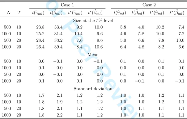
One possibility to get rid of the distorted standard errors of the ML estimator is to use the bootstrap. This approach has become very popular in applied work, and it will therefore be used in this paper. The particular algorithm used is taken from Cameron and Trivedi (1998), who make a very simple proposal, in which the dependent and independent variables are resampled in pairs.9 Some simulations of the resulting bootstrapped t-statistic based on
100 bootstrap replications are reported in Table 2. As expected, we see that the size of the bootstrapped test generally lies much closer to the 5% level than the size of the asymptotic test. Also, thet-statistics appear to be well centered around zero.
In summary, we find that the poisson ML show smaller bias than the two LS estimators considered and, at the same time, maintain relatively good size properties in small samples. Since the poisson ML with bootstrapped standard errors is now readily available through existing software packages such as STATA, it should be considered a feasible alternative to estimation by LS.
9Another possibility is to use the wild bootstrap, see Cameron and Trivedi (1998) for a discussion.
6 7 8 9 10 11 12 13 14 15 16 17 18 19 20 21 22 23 24 25 26 27 28 29 30 31 32 33 34 35 36 37 38 39 40 41 42 43 44 45 46 47 48 49 50 51 52 53 54 55 56 57 58 59 60
For Peer Review
4
An application to the 1995 EU enlargement
We have shown that log-linear LS estimation of the gravity model yields biased results. In this section, we demonstrate these findings by estimating the trade effects of the adhesion of Austria, Finland and Sweden to the EU in 1995. The sample that we use for this purpose cover the period 1992 to 2002 and consists of import data for EU and other developed countries from all trade partners except oil exporting countries and formerly planned economies in Central and Eastern Europe, as defined in Direction of Trade Statistics (International Monetary Fund, 2005). The GDP and population data comes from World Development Indicators (World Bank, 2005).
The estimated gravity equation can be written as
Mijt = exp(αij +µt+γ1Dit+γ2Djt+γ3Dijt)Yitβ1Yjtβ2Nitβ3Njtβ4vijt, (7)
or equivalently in its log-linear form
ln(Mijt) = αij +µt+γ1Dit+γ2Djt+γ3Dijt+β1ln(Yit) +β2ln(Yjt)
+ β3ln(Nit) +β4ln(Njt) + ln(vijt), (8)
whereMijt denotes the nominal imports of countryifrom country j,Yit and Yjt denote the
real GDP of the two countries, and Nit and Njt denote their population. The fixed effects
αij capture all types of unobserved country-pair specific heterogeneity that is constant over
time, while the time effectsµt capture all forms of time-varying heterogeneity that is shared
among the country pairs.
The dummy variables Dit, Djt and Dijt are key in this model. The variableDit equals one if countryi is a member of the EU at time t while country j belongs to the rest of the world. The second dummy variableDjt equals one if countryj is a member of the EU while
i belongs to the rest of the world. Similarly, Dijt equals one if both i and j are members
of the EU at time t. In other words, the three dummy variables take the value one for EU imports from the rest of the world, EU exports to the rest of the world and intra-EU trade, respectively.
The rest of the world is defined as all countries in the sample that are not members of the EU at any given time in the sample. This enables us to identify the effect of the enlargement on the trade of new EU members as opposed to the effect of changes in the size of the rest of the world. To appreciate this, note that if the rest of the world also included new members,
6 7 8 9 10 11 12 13 14 15 16 17 18 19 20 21 22 23 24 25 26 27 28 29 30 31 32 33 34 35 36 37 38 39 40 41 42 43 44 45 46 47 48 49 50 51 52 53 54 55 56 57 58 59 60
For Peer Review
the dummy variable Dit would capture not only the import effect on the new members but
also the effect of the change in the composition of the rest of the world, as the imports from the new members to the old ones would no longer be classified as imports from the rest of the world. A similar argument applies to the construction ofDjt.
A consequence of this definition of the rest of the world is that, since fixed effects absorb all heterogeneity that is constant over time, the trade effect for countries that have been members of the EU for the whole sample period cannot be identified. Thus, the dummy variables capture only the effect on countries that have changed their EU status at least one time. That is, the dummy variables capture the effect of the Austrian, Finnish and Swedish accession to the EU. Specifically,γ1 measures the trade diversion or changes in EU imports
from the rest of the world. Similarly,γ2 measures the effect on EU exports to the rest of the
world, sometimes called export diversion. Finally,γ3 measures trade creation, resulting from the increased intra-EU trade following the enlargement.
Economic integration should increase trade between countries integrating. Thus, we ex-pect the trade creation, as measured byγ3, to be positive. This effect can be separated into
pure trade creation, or increased trade due to lower prices on imports from the other countries in the EU, and trade diversion, which implies a shift in imports from more efficient producers in the rest of the world to less efficient producers within the EU. A negative sign onγ1 would
thus indicate trade diversion. Similarly, export diversion occurs if exports to the rest of the world decreases as a result of the integration process, but exports could also increase. The expected sign ofγ2 is therefore ambiguous.
The empirical results are contained in Table 3. It is seen that the enlargement of the EU induced significant trade diversion but no trade creation. This absence of trade creation is, however, not surprising since the new members were part of a free trade area with the EU prior to the membership. When joining the EU, the new members implemented the Common External Tariff, which changed the tariffs on their imports from the rest of the world. Note that the trade diversion effect is rather large in comparison to the trade creation effect. Although counterintuitive at first, one should keep in mind that several countries with preferential access to the EU market, such as those that joined the EU in 2004, have been excluded from our sample, so trade might have been diverted away from suppliers on the world market to suppliers with preferential access to the EU market. Moreover, taken as a fraction of total trade, the diversion effect is probably quite small since the estimation results
6 7 8 9 10 11 12 13 14 15 16 17 18 19 20 21 22 23 24 25 26 27 28 29 30 31 32 33 34 35 36 37 38 39 40 41 42 43 44 45 46 47 48 49 50 51 52 53 54 55 56 57 58 59 60
For Peer Review
only capture the effect on imports to Austria, Sweden and Finland and not changes in the total imports of the EU.
Even though the number of zeros is comparatively small in our sample, only 10%, when comparing the results obtained from the various estimators, we see that the difference can be substantial. In particular, for the GDP and population variables, the poisson ML estimates are typically larger than their LS counterparts. This finding is well in line with the Monte Carlo evidence suggesting that both LS estimators are downwards biased. Moreover, while the truncated LS estimator indicates that changes in GDP of importing countries does not effect imports, the ML estimator gives a more plausible estimate close to unity.
It should also be mentioned that the LS estimates of the GDP and population parameters appear to be rather unstable, and to a large extent dependent on the time period used, which is probably due to the fact that these variables seem to be quite highly correlated. On the other hand, the corresponding LS estimates of the effects of trade liberalization appear to be very robust, and show almost no variation between time periods. Similarly, all ML estimates seem vary robust to changes in the time period.
For the dummy variables, the differences are less marked. In particular, although the sign and significance of the estimates do not differ much, the magnitude of the estimates varies quite substantially. The LS estimator indicates that the trade diversion is twice as large as implied by the ML estimator and, while the LS estimate of the trade creation effect is slightly negative, it is positive for the ML estimator.
In summary, the results presented in this section highlight the importance of using appro-priate estimation techniques to be able to draw correct inference.
5
Conclusions
The gravity model has become a standard tool for evaluating policies affecting trade and it is widely used to assess the effects of preferential trade agreements and currency unions or to calculate trade potential, among other things. It is well known that the gravity model should be estimated by panel data to mitigate the bias due to failure to fully control for country heterogeneity. A very popular way to accomplish this is to first linearize the model by taking logarithms and then to apply the conventional fixed effects LS estimator.
In this paper, we argue that this approach is likely to be very misleading with severely biased estimates and t-statistics. There are two reasons for this. Firstly, since trade cannot
6 7 8 9 10 11 12 13 14 15 16 17 18 19 20 21 22 23 24 25 26 27 28 29 30 31 32 33 34 35 36 37 38 39 40 41 42 43 44 45 46 47 48 49 50 51 52 53 54 55 56 57 58 59 60
For Peer Review
be zero in the log-linearized model, all zeros must either be discarded or replaced by some arbitrary positive value, which induces a sample selection bias. Secondly, the heteroskedas-ticity inherent in the log-linear formulation of the gravity model can render the LS estimates both biased and inefficient. By contrast, being based on the gravity model in its original non-linear form, the fixed effects poisson ML estimator does not suffer from these weaknesses and is therefore expected to yield more accurate results.
Our assertion is verified by means of Monte Carlo simulations and illustrated via an application to the 1995 EU enlargement. The simulations show that the performance of the log-linear approach is likely to be so poor that it may not even be meaningful to interpret the results. On the other hand, the poisson ML estimator performs well with only a very small bias and good size accuracy in most cases. Still, in some data generating processes, the results show that the estimated standard errors can be downward biased. To alleviate this, we suggest using bootstrapped standard errors. The empirical application points to a significant difference between the estimators with respect to both the main explanatory variables and the trade effects of the 1995 EU enlargement, thus underlining the importance of using the proper estimation technique.
To conclude, we recommend not estimating the gravity model from its log-linear form. Instead, we propose estimating the model directly from its non-linear form using the fixed effects poisson ML estimator with bootstrapped standard error. Our proposal provide re-searchers with a simple framework for analyzing the gravity model while at the same time avoiding potential bias due to zero trade. This, together with the fact that the poisson ML estimator can now be implemented using many standard statistical software packages such as STATA, makes our proposal definitely seem worthwhile.
6 7 8 9 10 11 12 13 14 15 16 17 18 19 20 21 22 23 24 25 26 27 28 29 30 31 32 33 34 35 36 37 38 39 40 41 42 43 44 45 46 47 48 49 50 51 52 53 54 55 56 57 58 59 60
For Peer Review
T able 1: Sim ulated bias and tests size for the ML and LS estimators. Mean bias Size of the t -test at the 5% lev el δ Case N T b γ a ls bβ a ls b γ b ls bβ b ls b γml bβml b γ a ls bβ a ls b γ b ls bβ b ls b γml bβml 0 1 500 10 0 . 1 − 0 . 1 − 36 . 4 − 36 . 9 0 . 1 − 0 . 1 7 . 3 5 . 8 100 . 0 100 . 0 24 . 6 31 . 8 1000 10 0 . 0 0 . 0 − 36 . 5 − 36 . 8 − 0 . 1 − 0 . 1 6 . 6 5 . 8 100 . 0 100 . 0 25 . 6 32 . 2 500 20 0 . 1 0 . 1 − 36 . 5 − 36 . 7 0 . 1 0 . 2 6 . 2 6 . 1 100 . 0 100 . 0 24 . 1 33 . 4 1000 20 − 0 . 1 0 . 0 − 36 . 5 − 36 . 8 − 0 . 1 − 0 . 2 5 . 9 6 . 2 100 . 0 100 . 0 26 . 5 31 . 9 2 500 10 13 . 8 14 . 1 − 25 . 8 − 26 . 6 − 0 . 1 0 . 0 100 . 0 99 . 8 100 . 0 100 . 0 5 . 0 6 . 3 1000 10 13 . 8 14 . 2 − 25 . 8 − 26 . 5 0 . 1 0 . 1 100 . 0 100 . 0 100 . 0 100 . 0 3 . 7 4 . 4 500 20 13 . 8 14 . 1 − 25 . 8 − 26 . 6 0 . 0 0 . 0 100 . 0 100 . 0 100 . 0 100 . 0 6 . 1 4 . 8 1000 20 13 . 9 14 . 2 − 25 . 8 − 26 . 6 0 . 1 0 . 1 100 . 0 100 . 0 100 . 0 100 . 0 4 . 9 5 . 3 0 . 1 1 500 10 − 21 . 8 − 21 . 8 − 36 . 5 − 36 . 8 − 0 . 1 − 0 . 1 100 . 0 99 . 9 100 . 0 100 . 0 25 . 3 29 . 6 1000 10 − 21 . 9 − 21 . 8 − 36 . 6 − 36 . 8 − 0 . 1 − 0 . 1 100 . 0 100 . 0 100 . 0 100 . 0 23 . 9 29 . 5 500 20 − 21 . 9 − 21 . 9 − 36 . 6 − 36 . 8 − 0 . 1 − 0 . 1 100 . 0 100 . 0 100 . 0 100 . 0 27 . 1 31 . 3 1000 20 − 21 . 8 − 21 . 9 − 36 . 5 − 36 . 8 0 . 0 0 . 0 100 . 0 100 . 0 100 . 0 100 . 0 25 . 3 32 . 2 2 500 10 − 9 . 4 − 13 . 4 − 25 . 7 − 26 . 6 0 . 1 − 0 . 1 99 . 8 99 . 8 100 . 0 100 . 0 4 . 7 4 . 9 1000 10 − 9 . 5 − 13 . 5 − 25 . 8 − 26 . 6 0 . 0 − 0 . 1 100 . 0 100 . 0 100 . 0 100 . 0 5 . 5 4 . 9 500 20 − 9 . 4 − 13 . 4 − 25 . 8 − 26 . 6 0 . 0 − 0 . 1 100 . 0 100 . 0 100 . 0 100 . 0 5 . 6 4 . 5 1000 20 − 9 . 5 − 13 . 3 − 25 . 8 − 26 . 5 0 . 0 0 . 1 100 . 0 100 . 0 100 . 0 100 . 0 5 . 7 5 . 7 0 . 3 1 500 10 − 44 . 8 − 40 . 9 − 36 . 5 − 36 . 8 − 0 . 1 − 0 . 2 100 . 0 100 . 0 100 . 0 100 . 0 27 . 2 29 . 5 1000 10 − 44 . 7 − 41 . 0 − 36 . 5 − 36 . 8 0 . 0 − 0 . 2 100 . 0 100 . 0 100 . 0 100 . 0 26 . 6 34 . 3 500 20 − 44 . 6 − 40 . 9 − 36 . 5 − 36 . 8 0 . 1 0 . 1 100 . 0 100 . 0 100 . 0 100 . 0 28 . 8 33 . 2 1000 20 − 44 . 8 − 41 . 0 − 36 . 6 − 36 . 8 − 0 . 1 − 0 . 1 100 . 0 100 . 0 100 . 0 100 . 0 26 . 7 32 . 9 2 500 10 − 41 . 4 − 29 . 0 − 25 . 9 − 26 . 6 − 0 . 1 − 0 . 1 100 . 0 100 . 0 100 . 0 100 . 0 4 . 0 5 . 1 1000 10 − 41 . 4 − 28 . 9 − 25 . 8 − 26 . 6 0 . 0 0 . 1 100 . 0 100 . 0 100 . 0 100 . 0 6 . 1 3 . 9 500 20 − 41 . 4 − 29 . 2 − 25 . 8 − 26 . 7 0 . 0 − 0 . 1 100 . 0 100 . 0 100 . 0 100 . 0 5 . 3 5 . 5 1000 20 − 41 . 4 − 29 . 1 − 25 . 8 − 26 . 6 0 . 0 0 . 1 100 . 0 100 . 0 100 . 0 100 . 0 5 . 0 5 . 2 Notes : The value δ refers to the fraction of truncated observ ations, b γls and bβls refer to the LS estimates, and b γml and bβml refer to the p oisson ML estimates. Case 1 refers to the data generating pro cess with σ 2 ij = 1, while case 2 refers to the data generating pro cess with var( Mij t | Yij t ,D ij t ) = E ( Mij t | Yij t ,D ij t ). The rep orted bias results refer to the mean bias times 100. aThe LS estimator is based on truncating the sample. bThe LS estimator uses ln( Mij t + 1) as the dep enden t variable 6 7 8 9 10 11 12 13 14 15 16 17 18 19 20 21 22 23 24 25 26 27 28 29 30 31 32 33 34 35 36 37 38 39 40 41 42 43 44 45 46 47 48 49 50 51 52 53 54 55 56 57 58 59 60For Peer Review
Table 2: Simulation results for the bootstrapped ML t-test.
Case 1 Case 2
N T t(bγml) t(βbml) t∗(γbml) t∗(βbml) t(bγml) t(βbml) t∗(bγml) t∗(βbml)
Size at the 5% level
500 10 23.8 33.4 9.2 10.0 5.8 4.0 10.2 7.4 1000 10 25.2 31.4 10.4 9.6 4.6 5.8 10.0 7.2 500 20 28.4 33.2 7.6 9.6 5.0 6.6 7.8 10.0 1000 20 26.4 39.4 8.4 10.6 6.4 4.8 8.2 6.6 Mean 500 10 0.0 −0.1 0.0 −0.1 0.1 0.0 0.1 0.1 1000 10 0.1 0.0 0.0 0.0 0.0 0.0 0.0 0.0 500 20 0.0 −0.1 0.0 0.0 0.1 0.0 0.1 0.0 1000 20 0.1 0.0 0.1 0.0 0.0 −0.1 0.0 −0.1 Standard deviation 500 10 1.7 2.1 1.2 1.2 1.0 1.0 1.2 1.1 1000 10 1.8 1.9 1.2 1.2 1.0 1.0 1.2 1.1 500 20 1.8 2.1 1.1 1.2 1.0 1.1 1.1 1.1 1000 20 1.8 2.2 1.1 1.2 1.0 1.0 1.1 1.1
Notes: The valuest(bγml) andt(βbml) refer to the conventional asymptotic MLt-tests, while
t∗(bγ
ml) andt∗(βbml) refer to thir bootstrapped counterparts. See Table 1 for an explanation
of the remaining features of the table. 6 7 8 9 10 11 12 13 14 15 16 17 18 19 20 21 22 23 24 25 26 27 28 29 30 31 32 33 34 35 36 37 38 39 40 41 42 43 44 45 46 47 48 49 50 51 52 53 54 55 56 57 58 59 60
For Peer Review
Table 3: Empirical estimation results.Estimator LS LS poisson ML Dependent variable ln(Mijt) ln(Mijt+ 1) Mijt
β1 −0.091 0.229∗∗∗ 0.931∗∗∗ (0.191) (0.062) (0.173) β2 1.438∗∗∗ 0.820∗∗∗ 1.483∗∗∗ (0.084) (0.039) (0.110) β3 4.055∗∗∗ 1.765∗∗∗ 2.471∗∗∗ (0.612) (0.267) (0.629) β4 −1.275∗∗∗ −0.979∗∗∗ −0.580 (0.190) (0.074) (0.357) γ1 −0.403∗∗∗ −0.211∗∗∗ −0.232∗∗∗ (0.046) (0.016) (0.074) γ2 0.000 0.102∗∗∗ 0.041 (0.032) (0.023) (0.047) γ3 −0.002 0.033∗ 0.035 (0.025) (0.018) (0.034) No. of country-pairs 2719 2748 2719 No. of observations 32487 35600 35256
Notes: The numbers within the parantheses are the robust LS standard errors or the bootstrapped poisson ML standard errors. The superscripts (∗∗∗), (∗∗) and (∗) denote significance at the 1%, 5% and 10% levels,
respectively. 6 7 8 9 10 11 12 13 14 15 16 17 18 19 20 21 22 23 24 25 26 27 28 29 30 31 32 33 34 35 36 37 38 39 40 41 42 43 44 45 46 47 48 49 50 51 52 53 54 55 56 57 58 59 60
For Peer Review
References
Blundell, R., R. Griffth, and F. Windmeijer (2002). Individual effects and dynamics in count data models. Journal of Econometrics 108, 113–131.
Cameron, C. A., and P. K. Trivedi (1998). Regression analysis of count data. Cambridge. United Kingdom, Cambridge University Press.
Cheng, I.-H., and H. J. Wall (2005). Controlling heterogeneity in gravity models of trade and integration. Review of the Federal Reserve Bank of St. Louis 87, 49–63.
Cheng, I.-H., and Y.-Y. Tsai (2008). Estimating the staged effects of regional economic integration on trade volumes. Applied Economics 40, 383–393.
Hausman, J., B. H. Hall and Z. Griliches (1984). Econometric models for count data with an application to patents-R&D relationship. Econometrica 52, 909–938.
Helpman, E., M. Melitz and Y. Rubinstein (2008). Estimating trade flows: trading partners and trading volumes. Quarterly Journal of Economics 123, 441–487.
Gourieroux, C., A. Monfort and A. Trognon (1984). Pseudo maximum likelihood methods: theory. Econometrica 52, 681–700.
International Monetary Fund (2005). Direction of trade statistics, CD-Rom. International
Monetary Fund, Washington DC.
Kyriazidou, E. (1997). Estimation of a panel data sample selection model. Econometrica 65, 1335–1364.
Silva, J. M. C. S., and S. Tenereyro (2006). The log of gravity. Review of Economics and
Statistics 88, 641–658.
Winkelman, R. (2008). Econometric analysis of count data. Fifth edition, Springer, Berlin-Hidelberg.
Wooldridge, J. M. (2002). Econometric analysis of cross section and panel data. Cambridge, MA, MIT Press.
World Bank (2005). World development indicators, CD-Rom. The World Bank, Washington DC. 6 7 8 9 10 11 12 13 14 15 16 17 18 19 20 21 22 23 24 25 26 27 28 29 30 31 32 33 34 35 36 37 38 39 40 41 42 43 44 45 46 47 48 49 50 51 52 53 54 55 56 57 58 59 60