After teaching mathematical statistics for several years using chalk on a black-board (and, later, smelly “dry erase markers” on a whiteblack-board) mostly doing proofs of theorems, I decided to lecture from computer slides that provide an outline of the “big picture”. Rather than spend class time “doing” proofs that are given in standard texts, I decided that time would be better spent discussing the material from a different, higher-level perspective.
While lecturing from canned slides, I cannot, however, ignore certain de-tails of proofs and minutiae of examples. But what dede-tails and which minutiae? To be effective, my approach depends on an understanding between students and the instructor, an understanding that is possibly implicit. I lecture; but I ask “what is ... ?” and “why is ... ?”; and I encourage students to ask “what is ... ?” and “why is ... ?”. I adopt the attitude that there are many things that I don’t know, but if there’s something that I wonder about, I’ll admit ignorance and pursue the problem until I’ve attained some resolution. I encourage my students to adopt a similar attitude.
I am completely dissatisfied with a class that sits like stumps on a log when I ask “what is ... ?” or “why is ... ?” during a lecture. What can I say? After writing class slides (in LATEX 2ε, of course), mostly in bullet form, I began writing text around the bullets, and I put the notes on the class website. Later I decided that a single document with a fairly extensive subject index (see pages ?? through ??) would be useful to serve as a companion for the study of mathematical statistics. The other big deal about this document is the internal links, which of course is not something that can be done with a hardcopy book. (One thing I must warn you about is that there is a (known) bug in the LATEX package hyperref; if the referenced point happens to occur at the top of a page, the link takes you to the previous page – so if you don’t see what you expect, try going to the next page.)
Another characteristic of this document that results from the nature of its origin, as well as from the medium itself (electronic) is its length. A long book doesn’t use any more paper or “kill any more trees” than a short book. Usually, however, we can expect the density of “importance” in a short document to be greater than that in a long document. If I had more time I could make this book shorter by prioritizing its content, and I may do that someday.
Several sections are incomplete and several proofs are omitted. Also, I plan to add more examples.I just have not had time to type up the material.
I do not recommend that you print these notes. First of all, they are evolv-ing, so a printed version is just a snapshot. Secondly, the PDF file contains active internal links, so navigation is easy. (For versions without active links, I try to be friendly to the reader by providing page numbers with most internal references.)
This document is directed toward students for whom the theory of statis-tics is or will become an important part of their lives. Obviously, such students should be able to work through the details of “hard” proofs and derivations; that is, students should master the fundamentals of mathematical statistics. In addition, students at this level should acquire, or begin acquiring, a deep appreciation for the field, including its historical development and its rela-tion to other areas of mathematics and science generally; that is, students should master the fundamentals of the broader theory of statistics. Some of the chapter endnotes are intended to help students gain such an appreciation by leading them to background sources and also by making more subjective statements than might be made in the main body.
It is important to understand the intellectual underpinnings of our science. There are certain principles(such as sufficiency, for example) that guide our approaches to statistical inference. There are various general approaches (see page239) that we follow. Within these general approaches there are a number of specific methods (see page240). The student should develop an appreciation for the relations between principles, approaches, and methods.
This book on mathematical statistics assumes a certain amount of back-ground in mathematics. Following the final chapter on mathematical statistics Chapter 8, there is Chapter0 on “statistical mathematics” (that is, mathe-matics with strong relevance to statistical theory) that provides much of the general mathematical background for probability and statistics. The mathe-matics in this chapter is prerequisite for the main part of the book, and it is hoped that the reader already has command of the material; otherwise, Chapter0can be viewed as providing “just in time” mathematics. Chapter0 grew (and is growing) recursively. Every time I add material, it seems that I need to add some background for the new material. This is obviously a game one cannot win.
The objective in the discussion of probability theory in Chapter 1, as in that of the other mathematical background, is to provide some of the most relevant material for statistics, which is the real topic of this text. Chapter2is also on probability, but the focus is on the applications in statistics. In that chapter, I address some important properties of probability distributions that determine properties of statistical methods when applied to observations from those distributions.
Chapter 3 covers many of the fundamentals of statistics. It provides an overview of the topics that will be addressed in more detail in Chapters 4 through8.
This document is organized in the order in which I cover the topics (more-or-less!). Material from Chapter 0 may be covered from time to time during the course, but I generally expect this chapter to be used for reference as needed for the statistical topics being covered.
The primary textbooks I have used in the past few years are Shao (2003),Lehmann and Casella(1998), and Lehmann (1986) (the precursor to Lehmann and Romano(2005)). At various places in this document, references are given to the related sections ofShao(2003) (“MS2”),Lehmann and Casella (1998) (“TPE2”), andLehmann and Romano(2005) (“TSH3”). These texts state all of the important theorems, and in most cases, provide the proofs. They are also replete with examples. Full bibliographic citations for these references, as well as several other resources are given in the bibliography beginning on page873.
It is of course expected that the student will read the primary textbook, as well as various other texts, and to work through all proofs and examples in the primary textbook.As a practical matter, obviously, even if I attempted to cover all of these in class, there just is not enough class time to do it.
The purpose of this evolving document is not just to repeat all of the material in those other texts. Its purpose, rather, is to provide some additional background material, and to serve as an outline and a handy reference of terms and concepts. The nature of the propositions vary consider-ably; in some cases, a fairly trivial statement will be followed by a proof, and in other cases, a rather obtuse statement will not be supported by proof. In all cases, the student should understand why the statement is true (or, if it’s not, immediately send me email to let me know of the error!). More importantly, the student should understand why it’s relevant.
Each student should read this and other texts and work through the proofs and examples at a rate that matches the individual student’s understanding of the individual problem. What one student thinks is rather obtuse, another student comprehends quickly, and then the tables are turned when a different problem is encountered. There is a lot of lonely work required, and this is why lectures that just go through the details are often not useful.
and yet without implying any claim of originality. (A notable exception is Graham et al. (1994).) My book is not intended to present new and origi-nal work, and it follows the time-honored tradition of reusing examples and exercises from long-forgotten sources.
Notation
Adoption of notation is an overhead in communication. I try to minimize that overhead by using notation that is “standard”, and using it locally consis-tently.
Examples of sloppy notation abound in mathematical statistics. Functions seem particularly susceptible to abusive notation. It is common to see “f(x)” and “f(y)” used in the same sentence to represent two different functions. (These often represent two different PDFs, one for a random variableX and the other for a random variableY. When I want to talk about two different things, I denote them by different symbols, so when I want to talk about two different PDFs, I often use notation such as “fX(·)” and “fY(·)”. If x=y, which is of course very different from saying X = Y, then fX(x) =fX(y); however, fX(x)6=fY(x) in general.)
For a function and a value of a function, there is a certain amount of ambiguity that is almost necessary. I generally try to use notation such as “f(x)” or “Y(ω)” to denote the value of the function f at xor Y at ω, and I use “f”, “f(·)”, or “Y” to denote the function itself (although occasionally, I do use “f(x)” to represent the function — notice the word “try” in this discussion).
If in the notation “f(x)”, “x” denotes an element of a set A, andB ⊆A (that is,B is a set of the same kinds of elements asA), then “f(B)” does not make much sense. For the image ofB under f, I use “f[B]”.
I also freely use the notation f−1(y) or f−1[B] to denote the preimage, whether or notf−1 is actually a function; that is, whether or notf is invert-ible.
There are two other areas in which my notation may be slightly different from common notation. First, to designate the open interval between the real numbers a < b, I use the Bourbaki notation “]a, b[”. (I eschew most of the weird Bourbaki notation, however. This particular notation is also used in my favorite book on analysis, Hewitt and Stromberg (1965).) Second, I do not use any special notation, such as boldface, for vectors; thus,xmay represent a scalar or a vector.
All vectors are “column vectors”. This is only relevant in vector-vector or vector-matrix operations, and has nothing to do with the way we represent a vector. It is far more convenient to represent the vectorxas
x= (x1, . . . , xd)
x=
x1 .. . xd
,
and there is certainly no need to use the silly notation
x= (x1, . . . , xd)T.
A vector is not a matrix.
There are times, however, when a vector may be treated like a matrix in certain operations. In such cases, the vector is treated as a matrix with one column.
AppendixCprovides a list of the common notation that I use. The reader is encouraged to look over that list both to see the notation itself and to get some idea of the objects that I discuss.
Solving Problems
The main ingredient for success in a course in mathematical statistics is the ability to work problems. The only way to enhance one’s ability to work problems is to work problems. It is not sufficient to read, to watch, or to hear solutions to problems.One of the most serious mistakes students make in courses in mathematical statistics is to work through a solution that somebody else has done and to think they have worked the problem.
While sometimes it may not be possible to solve a given problem, rather than looking for a solution that someone else has come up with, it is much better to stop with a partial solution or a hint and then sometime later return to the effort of completing the solution.Studying a problem without its solution is much more worthwhile than studying the solution to the problem.
Do you need to see a solution to a problem that you have solved? Except in rare cases, if you have solved a problem, you know whether or not your purported solution is correct. It is like a Sudoku puzzle; although solutions to these are always published in the back of the puzzle book or in a later edition of the medium, I don’t know what these are for. If you have solved the puzzle you know that your solution is correct. If you cannot solve it, I don’t see any value in looking at the solution. It’s not going to make you a better Sudoku solver. (Sudoku is different from crossword puzzles, another of my pastimes. Seeing the solution or partial solution to a crossword puzzle can make you a better crossword solver.) There is an important difference in Sudoku puzzles and mathematical problems. In Sudoku puzzles, there is only one correct solution. In mathematical problems, there may be more than one way to solve a problem, so occasionally it is worthwhile to see someone else’s solution.
This means working on this stuff for about 40 hours a week for 5 years. This is approximately the amount of work that a student should do for receipt of a PhD degree (preferably in less than 5 years).
Many problems serve as models of “standard operations” for solving other problems. Some problems should become “easy pieces”.
Standard Operations
There are a number of operations and mathematical objects that occur over and over in deriving results or in proving propositions. These operations are sometimes pejoratively called “tricks”. In some sense, perhaps they are; but it is useful to identify these operations outside of the context of a specific application. Some of these standard operations and useful objects are listed in Section 0.0.9on page676.
Easy Pieces
I recommend that all students develop a list of easy pieces. These are proposi-tions or examples and counterexamples that the student can state and prove or describe and work throughwithout resort to notes. An easy piece is some-thing that is important in its own right, but also may serve as a model or template for many other problems. A student should attempt to accumulate a large bag of easy pieces. If development of this bag involves some memo-rization, that is OK, but things should just naturally get into the bag in the process of working problems and observing similarities among problems — and by seeing the same problem over and over.
Some examples of easy pieces are
• State and prove the information inequality (CRLB) for ad-vector param-eter. (Get the regularity conditions correct.)
• Give an example to distinguish the asymptotic bias from the limiting bias. • State and prove Basu’s theorem.
• Give an example of a function of some parameter in some family of distri-butions that is not U-estimable.
• A statement of the Neyman-Pearson Lemma (with or without the ran-domization) and its proof.
Some easy pieces in the background area of “statistical mathematics” are
• LetC be the class of all closed intervals in IR. Show that σ(C) = B(IR) (the real Borelσ-field).
• Define induced measure and prove that it is a measure. That is, prove: If (Ω,F, ν) is a measure space and (Λ,G) is a measurable space, andf is a function from Ω to Λ that is measurable with respect toF/G, thenν◦f−1 is a measure with domainG.
• State and prove Fatou’s lemma conditional on a sub-σ-field.
Make your own list of easy pieces.
Relevance and Boundaries
For any proposition or example, you should have a clear understanding ofwhy
the proposition or example is important. Where is it subsequently used? Is it used to prove something else important, or does it justify some statistical procedure?
Propositions and definitions have boundaries; that is, they apply to a spe-cific situation. You should look at the “edges” or “boundaries” of the hypothe-ses. What would happen if you were to remove one or more assumptions? (This is the idea behind counterexamples.) What would happen if you make stronger assumptions?
“It is clear” and “It can be shown”
I tend to use the phrase “it is clear ...” often. (I only realized this recently, because someone pointed it out to me.) When I say “it is clear ...”, I expect the reader to agree with me actively, not passively.
I use this phrase only when the statement is “clearly” true to me. I must admit, however, sometimes when I read the statement a few weeks later, it’s not very clear! It may require many minutes of difficult reasoning. In any event, the reader should attempt to supply the reasoning for everything that I say is clear.
I also use the phrase “it can be shown ...” in connection with a fact (the-orem) whose proof at that point would be distracting, or else whose proof I just don’t want to write out. (In later iterations of this document, however, I may decide to give the proof.) A statement of fact preceded by the phrase “it can be shown”, is likely to require more thought or background information than a statement preceded by the phrase “it is clear”, although this may be a matter of judgement.
Study of mathematical statistics at the level appropriate for this document is generally facilitated by reference to a number of texts and journal articles; and I assume that the student does refer to various sources.
My Courses
Chapters 1 and 2 are on “probability”, some of their focus is more on what is usually covered in “statistics” courses, such as families of distributions, in particular, the exponential class of families.
My notes on these courses are available at
http://mason.gmu.edu/~jgentle/csi9723/
Acknowledgements
A work of this size is bound to have some errors (at least if I have anything to do with it!). Errors must first be detected and then corrected.
I would appreciate any feedback – errors, comments, or suggestions. Email me [email protected]
Fairfax County, Virginia James E. Gentle
Preface . . . v
1 Probability Theory . . . 1
1.1 Some Important Probability Definitions and Facts . . . 3
1.1.1 Probability and Probability Distributions. . . 4
1.1.2 Random Variables. . . 8
1.1.3 Definitions and Properties of Expected Values . . . 25
1.1.4 Relations among Random Variables. . . 35
1.1.5 Entropy. . . 40
1.1.6 Fisher Information . . . 42
1.1.7 Generating Functions . . . 42
1.1.8 Characteristic Functions. . . 45
1.1.9 Functionals of the CDF; Distribution “Measures”. . . 51
1.1.10 Transformations of Random Variables. . . 54
1.1.11 Decomposition of Random Variables. . . 60
1.1.12 Order Statistics. . . 62
1.2 Series Expansions . . . 65
1.2.1 Asymptotic Properties of Functions. . . 65
1.2.2 Expansion of the Characteristic Function. . . 66
1.2.3 Cumulants and Expected Values . . . 66
1.2.4 Edgeworth Expansions in Hermite Polynomials. . . 67
1.2.5 The Edgeworth Expansion. . . 68
1.3 Sequences of Spaces, Events, and Random Variables . . . 69
1.3.1 The Borel-Cantelli Lemmas. . . 72
1.3.2 Exchangeability and Independence of Sequences. . . 74
1.3.3 Types of Convergence. . . 75
1.3.4 Weak Convergence in Distribution. . . 85
1.3.5 Expectations of Sequences; Sequences of Expectations. . 89
1.3.6 Convergence of Functions. . . 91
1.3.8 Asymptotic Expectation. . . 100
1.4 Limit Theorems . . . 101
1.4.1 Laws of Large Numbers . . . 102
1.4.2 Central Limit Theorems for Independent Sequences. . . . 104
1.4.3 Extreme Value Distributions. . . 108
1.4.4 Other Limiting Distributions. . . 109
1.5 Conditional Probability . . . 110
1.5.1 Conditional Expectation: Definition and Properties . . . . 110
1.5.2 Some Properties of Conditional Expectations . . . 112
1.5.3 Projections . . . 115
1.5.4 Conditional Probability and Probability Distributions. . 119
1.6 Stochastic Processes . . . 121
1.6.1 Probability Models for Stochastic Processes. . . 125
1.6.2 Continuous Time Processes. . . 126
1.6.3 Markov Chains. . . 126
1.6.4 L´evy Processes and Brownian Motion. . . 129
1.6.5 Brownian Bridges . . . 130
1.6.6 Martingales. . . 130
1.6.7 Empirical Processes and Limit Theorems. . . 133
Notes and Further Reading. . . 137
Exercises . . . 145
2 Distribution Theory and Statistical Models. . . 155
2.1 Complete Families. . . 162
2.2 Shapes of the Probability Density . . . 163
2.3 “Regular” Families . . . 168
2.3.1 The Fisher Information Regularity Conditions . . . 168
2.3.2 The Le Cam Regularity Conditions. . . 169
2.3.3 Quadratic Mean Differentiability . . . 169
2.4 The Exponential Class of Families. . . 169
2.4.1 The Natural Parameter Space of Exponential Families . 173 2.4.2 The Natural Exponential Families. . . 173
2.4.3 One-Parameter Exponential Families. . . 173
2.4.4 Discrete Power Series Exponential Families . . . 175
2.4.5 Quadratic Variance Functions. . . 175
2.4.6 Full Rank and Curved Exponential Families . . . 175
2.4.7 Properties of Exponential Families. . . 176
2.5 Parametric-Support Families. . . 177
2.6 Transformation Group Families . . . 178
2.6.1 Location-Scale Families . . . 179
2.6.2 Invariant Parametric Families. . . 182
2.7 Infinitely Divisible and Stable Families. . . 183
2.8 Families of Distributions with Heavy Tails. . . 184
2.9 The Family of Normal Distributions . . . 185
2.9.2 Functions of Normal Random Variables . . . 187
2.9.3 Characterizations of the Normal Family of Distributions189 2.10 Generalized Distributions and Mixture Distributions. . . 192
2.10.1 Truncated and Censored Distributions . . . 192
2.10.2 Mixture Families. . . 194
2.10.3 Skewed Distributions . . . 195
2.10.4 Flexible Families of Distributions Useful in Modeling. . . 196
2.11 Multivariate Distributions . . . 198
2.11.1 Marginal Distributions. . . 198
2.11.2 Elliptical Families . . . 198
2.11.3 Higher Dimensions . . . 199
Notes and Further Reading. . . 199
Exercises . . . 201
3 Basic Statistical Theory . . . 205
3.1 Inferential Information in Statistics . . . 211
3.1.1 Statistical Inference: Point Estimation . . . 215
3.1.2 Sufficiency, Ancillarity, Minimality, and Completeness. . 221
3.1.3 Information and the Information Inequality. . . 229
3.1.4 “Approximate” Inference. . . 235
3.1.5 Statistical Inference in Parametric Families. . . 235
3.1.6 Prediction. . . 236
3.1.7 Other Issues in Statistical Inference. . . 236
3.2 Statistical Inference: Approaches and Methods . . . 239
3.2.1 Likelihood. . . 241
3.2.2 The Empirical Cumulative Distribution Function. . . 246
3.2.3 Fitting Expected Values. . . 250
3.2.4 Fitting Probability Distributions . . . 253
3.2.5 Estimating Equations. . . 254
3.2.6 Summary and Preview. . . 258
3.3 The Decision Theory Approach to Statistical Inference . . . 259
3.3.1 Decisions, Losses, Risks, and Optimal Actions. . . 259
3.3.2 Approaches to Minimizing the Risk. . . 267
3.3.3 Admissibility . . . 270
3.3.4 Minimaxity. . . 274
3.3.5 Summary and Review. . . 276
3.4 Invariant and Equivariant Statistical Procedures. . . 279
3.4.1 Formulation of the Basic Problem . . . 280
3.4.2 Optimal Equivariant Statistical Procedures . . . 284
3.5 Probability Statements in Statistical Inference . . . 290
3.5.1 Tests of Hypotheses . . . 290
3.5.2 Confidence Sets . . . 296
3.6 Variance Estimation . . . 301
3.6.1 Jackknife Methods. . . 301
3.6.3 Substitution Methods. . . 304
3.7 Applications . . . 305
3.7.1 Inference in Linear Models. . . 305
3.7.2 Inference in Finite Populations. . . 305
3.8 Asymptotic Inference . . . 306
3.8.1 Consistency . . . 307
3.8.2 Asymptotic Expectation. . . 310
3.8.3 Asymptotic Properties and Limiting Properties . . . 311
3.8.4 Properties of Estimators of a Variance Matrix. . . 316
Notes and Further Reading. . . 317
Exercises . . . 322
4 Bayesian Inference. . . 325
4.1 The Bayesian Paradigm . . . 326
4.2 Bayesian Analysis . . . 331
4.2.1 Theoretical Underpinnings. . . 331
4.2.2 Regularity Conditions for Bayesian Analyses. . . 334
4.2.3 Steps in a Bayesian Analysis. . . 335
4.2.4 Bayesian Inference. . . 344
4.2.5 Choosing Prior Distributions. . . 346
4.2.6 Empirical Bayes Procedures . . . 352
4.3 Bayes Rules . . . 352
4.3.1 Properties of Bayes Rules . . . 353
4.3.2 Equivariant Bayes Rules. . . 354
4.3.3 Bayes Estimators with Squared-Error Loss Functions . . 354
4.3.4 Bayes Estimation with Other Loss Functions. . . 359
4.3.5 Some Additional (Counter)Examples. . . 361
4.4 Probability Statements in Statistical Inference . . . 361
4.5 Bayesian Testing . . . 362
4.5.1 A First, Simple Example. . . 363
4.5.2 Loss Functions. . . 364
4.5.3 The Bayes Factor . . . 366
4.5.4 Bayesian Tests of a Simple Hypothesis . . . 370
4.5.5 Least Favorable Prior Distributions. . . 372
4.6 Bayesian Confidence Sets. . . 372
4.6.1 Credible Sets . . . 372
4.6.2 Highest Posterior Density Credible sets . . . 373
4.6.3 Decision-Theoretic Approach . . . 373
4.6.4 Other Optimality Considerations. . . 374
4.7 Computational Methods in Bayesian Inference . . . 377
Notes and Further Reading. . . 380
5 Unbiased Point Estimation . . . 389
5.1 Uniformly Minimum Variance Unbiased Point Estimation. . . 392
5.1.1 Unbiased Estimators of Zero. . . 392
5.1.2 Optimal Unbiased Point Estimators . . . 393
5.1.3 Unbiasedness and Squared-Error Loss; UMVUE. . . 393
5.1.4 Other Properties of UMVUEs. . . 398
5.1.5 Lower Bounds on the Variance of Unbiased Estimators. 399 5.2 U-Statistics. . . 404
5.2.1 Expectation Functionals and Kernels . . . 404
5.2.2 Kernels and U-Statistics. . . 406
5.2.3 Properties of U-Statistics. . . 411
5.3 Asymptotically Unbiased Estimation. . . 414
5.3.1 Method of Moments Estimators. . . 416
5.3.2 Ratio Estimators. . . 417
5.3.3 V-Statistics. . . 417
5.3.4 Estimation of Quantiles . . . 418
5.4 Asymptotic Efficiency. . . 418
5.4.1 Asymptotic Relative Efficiency. . . 419
5.4.2 Asymptotically Efficient Estimators. . . 419
5.5 Applications . . . 423
5.5.1 Estimation in Linear Models. . . 423
5.5.2 Estimation in Survey Samples of Finite Populations . . . 438
Notes and Further Reading. . . 442
Exercises . . . 443
6 Statistical Inference Based on Likelihood . . . 445
6.1 The Likelihood Function and Its Use in Statistical Inference . . 445
6.2 Maximum Likelihood Parametric Estimation. . . 448
6.2.1 Definition and Examples . . . 449
6.2.2 Finite Sample Properties of MLEs. . . 457
6.2.3 The Score Function and the Likelihood Equations . . . 463
6.2.4 Finding an MLE . . . 465
6.3 Asymptotic Properties of MLEs, RLEs, and GEE Estimators . 481 6.3.1 Asymptotic Distributions of MLEs and RLEs . . . 481
6.3.2 Asymptotic Efficiency of MLEs and RLEs . . . 481
6.3.3 Inconsistent MLEs. . . 484
6.3.4 Properties of GEE Estimators. . . 486
6.4 Application: MLEs in Generalized Linear Models . . . 487
6.4.1 MLEs in Linear Models . . . 487
6.4.2 MLEs in Generalized Linear Models . . . 491
6.5 Variations on the Likelihood . . . 498
6.5.1 Quasi-likelihood Methods. . . 498
6.5.2 Nonparametric and Semiparametric Models. . . 499
Notes and Further Reading. . . 502
7 Statistical Hypotheses and Confidence Sets. . . 507
7.1 Statistical Hypotheses. . . 508
7.2 Optimal Tests. . . 514
7.2.1 The Neyman-Pearson Fundamental Lemma. . . 517
7.2.2 Uniformly Most Powerful Tests. . . 520
7.2.3 Unbiasedness of Tests. . . 523
7.2.4 UMP Unbiased (UMPU) Tests. . . 524
7.2.5 UMP Invariant (UMPI) Tests. . . 525
7.2.6 Equivariance, Unbiasedness, and Admissibility . . . 527
7.2.7 Asymptotic Tests. . . 527
7.3 Likelihood Ratio Tests, Wald Tests, and Score Tests . . . 528
7.3.1 Likelihood Ratio Tests . . . 528
7.3.2 Wald Tests . . . 530
7.3.3 Score Tests . . . 530
7.3.4 Examples . . . 531
7.4 Nonparametric Tests. . . 535
7.4.1 Permutation Tests. . . 535
7.4.2 Sign Tests and Rank Tests. . . 536
7.4.3 Goodness of Fit Tests. . . 536
7.4.4 Empirical Likelihood Ratio Tests. . . 536
7.5 Multiple Tests . . . 536
7.6 Sequential Tests. . . 538
7.6.1 Sequential Probability Ratio Tests. . . 539
7.6.2 Sequential Reliability Tests. . . 539
7.7 The Likelihood Principle and Tests of Hypotheses . . . 539
7.8 Confidence Sets . . . 541
7.9 Optimal Confidence Sets . . . 546
7.9.1 Most Accurate Confidence Set . . . 546
7.9.2 Unbiased Confidence Sets . . . 547
7.9.3 Equivariant Confidence Sets . . . 549
7.10 Asymptotic Confidence sets. . . 550
7.11 Bootstrap Confidence Sets. . . 552
7.12 Simultaneous Confidence Sets. . . 557
7.12.1 Bonferroni’s Confidence Intervals. . . 557
7.12.2 Scheff´e’s Confidence Intervals . . . 558
7.12.3 Tukey’s Confidence Intervals. . . 558
Notes and Further Reading. . . 558
Exercises . . . 559
8 Nonparametric and Robust Inference. . . 561
8.1 Nonparametric Inference . . . 561
8.2 Inference Based on Order Statistics . . . 563
8.2.1 Central Order Statistics. . . 563
8.2.2 Statistics of Extremes. . . 564
8.3.1 General Methods for Estimating Functions . . . 567
8.3.2 Pointwise Properties of Function Estimators . . . 569
8.3.3 Global Properties of Estimators of Functions. . . 572
8.4 Semiparametric Methods and Partial Likelihood. . . 576
8.4.1 The Hazard Function . . . 577
8.4.2 Proportional Hazards Models . . . 578
8.5 Nonparametric Estimation of PDFs. . . 579
8.5.1 Nonparametric Probability Density Estimation. . . 579
8.5.2 Histogram Estimators. . . 582
8.5.3 Kernel Estimators. . . 590
8.5.4 Choice of Window Widths. . . 595
8.5.5 Orthogonal Series Estimators . . . 596
8.6 Perturbations of Probability Distributions . . . 597
8.7 Robust Inference . . . 602
8.7.1 Sensitivity of Statistical Functions. . . 604
8.7.2 Robust Estimators . . . 608
Notes and Further Reading. . . 609
Exercises . . . 610
0 Statistical Mathematics. . . 613
0.0 Some Basic Mathematical Concepts. . . 616
0.0.1 Sets . . . 616
0.0.2 Sets and Spaces. . . 621
0.0.3 Binary Operations and Algebraic Structures . . . 629
0.0.4 Linear Spaces. . . 634
0.0.5 The Real Number System . . . 640
0.0.6 The Complex Number System . . . 660
0.0.7 Monte Carlo Methods. . . 663
0.0.8 Mathematical Proofs. . . 673
0.0.9 Useful Mathematical Tools and Operations . . . 676
Notes and References for Section 0.0. . . 688
Exercises for Section 0.0. . . 689
0.1 Measure, Integration, and Functional Analysis . . . 692
0.1.1 Basic Concepts of Measure Theory . . . 692
0.1.2 Functions and Images. . . 701
0.1.3 Measure. . . 704
0.1.4 Sets in IR and IRd . . . 713
0.1.5 Real-Valued Functions over Real Domains. . . 720
0.1.6 Integration . . . 726
0.1.7 The Radon-Nikodym Derivative. . . 739
0.1.8 Function Spaces. . . 740
0.1.9 LpReal Function Spaces . . . 741
0.1.10 Distribution Function Spaces . . . 754
0.1.11 Transformation Groups . . . 754
0.1.13 Functionals. . . 759
Notes and References for Section 0.1. . . 761
Exercises for Section 0.1. . . 762
0.2 Stochastic Processes and the Stochastic Calculus . . . 765
0.2.1 Stochastic Differential Equations . . . 765
0.2.2 Integration with Respect to Stochastic Differentials. . . . 775
Notes and References for Section 0.2. . . 780
0.3 Some Basics of Linear Algebra . . . 781
0.3.1 Inner Products, Norms, and Metrics . . . 781
0.3.2 Matrices and Vectors . . . 782
0.3.3 Vector/Matrix Derivatives and Integrals. . . 801
0.3.4 Optimization of Functions. . . 811
0.3.5 Vector Random Variables. . . 816
0.3.6 Transition Matrices. . . 818
Notes and References for Section 0.3. . . 821
0.4 Optimization . . . 822
0.4.1 Overview of Optimization . . . 822
0.4.2 Alternating Conditional Optimization. . . 827
0.4.3 Simulated Annealing. . . 829
Notes and References for Section 0.4. . . 832
Appendices
A Important Probability Distributions. . . 835B Useful Inequalities in Probability . . . 845
B.1 Preliminaries. . . 845
B.2 Pr(X ∈Ai) and Pr(X ∈ ∪Ai) or Pr(X ∈ ∩Ai) . . . 846
B.3 Pr(X ∈A) and E(f(X)). . . 847
B.4 E(f(X)) and f(E(X)) . . . 849
B.5 E(f(X, Y)) and E(g(X)) and E(h(Y)) . . . 852
B.6 V(Y) and V E(Y|X). . . 855
B.7 Multivariate Extensions . . . 855
Notes and Further Reading. . . 856
C Notation and Definitions . . . 857
C.1 General Notation. . . 857
C.2 General Mathematical Functions and Operators . . . 860
C.3 Sets, Measure, and Probability. . . 866
C.4 Linear Spaces and Matrices. . . 868
References. . . 873
Probability Theory
Probability theory provides the basis for mathematical statistics.
Probability theory has two distinct elements. One is just a special case of measure theory and can be approached in that way. For this aspect, the presentation in this chapter assumes familiarity with the material in Section0.1beginning on page692. This aspect is “pure” mathematics. The other aspect of probability theory is essentially built on a gedanken experiment involving drawing balls from an urn that contains balls of different colors, and noting the colors of the balls drawn. In this aspect of probability theory, we may treat “probability” as a primitive (that is, undefined) concept. In this line of development, we relate “probability” informally to some notion of long-term frequency or to expectations or beliefs relating to the types of balls that will be drawn. Following some additional axiomatic developments, however, this aspect of probability theory is also essentially “pure” mathematics.
Because it is just mathematics, in probability theoryper se, we do not ask “what do you think is the probability that ...?” Given an axiomatic framework, one’s beliefs are irrelevant, whether probability is a measure or is a primitive concept. In statistical theory or applications, however, we may ask questions about “beliefs”, and the answer(s) may depend on deep philosophical consid-erations in connecting the mathematical concepts of probability theory with decisions about the “real world”. This may lead to a different definition of
probability. For example,Lindley and Phillips(1976), page 115, state “Proba-bility is a relation between you and the external world, expressing your opinion of some aspect of that world...” I am sure that an intellectually interesting theory could be developed based on ways of “expressing your opinion[s]”, but I will not use “probability” in this way; rather, throughout this book, I will use the term probabilityas a measure(see Definition0.1.10, page704). For spe-cific events in a given application, of course, certain values of the probability measure may be assigned based on “opinions”, “beliefs”, or whatever.
emphasis] of occurrence of events under large-scale repetition of uniform con-ditions.” (See a more complete quotation on page143.)
Ranks of Mathematical Objects
In probability theory we deal with various types of mathematical objects. We would like to develop concepts and identify properties that are indepen-dent of the type of the underlying objects, but that is not always possible. Occasionally we will find it necessary to discuss scalar objects, rank one ob-jects (vectors), and rank two obob-jects (matrices) separately. In general, most degree-one properties, such as expectations of linear functions, can be consid-ered uniformly across the different types of mathematical objects. Degree-two properties, such as variances, however, must usually be considered separately for scalars, vectors, and matrices.
Overview of Chapter
This chapter covers important topics in probability theory at a fairly fast pace. Some of the material in this chapter, such as the properties of certain families of distributions, is often considered part of “mathematical statistics”, rather than a part of probability theory. Unless the interest is in use ofdata
for describing a distribution or for making inferences about the distribution, however, the study of properties of the distribution is part of probability theory, rather than statistics.
We begin in Section 1.1 with statements of definitions and some basic properties. The initial development of this section parallels the first few sub-sections of Section 0.1for more general measures, and then the development of expectations depends on the results of Section 0.1.6for integration.
Sections1.3and1.4are concerned with sequences of independent random variables. The limiting properties of such sequences are important. Many of the limiting properties can be studied using expansions in power series, which is the topic of Section 1.2.
In the next chapter, beginning on page155, I identify and describe useful classes of probability distributions. These classes are important because they are good models of observable random phenomena, and because they are easy to work with. The properties of various statistical methods discussed in subsequent chapters depend on the underlying probability model, and some of the properties of the statistical methods can be worked out easily for particular models discussed in Chapter 2.
1.1 Some Important Probability Definitions and Facts
A probability distribution is built from a measure space in which the measure is a probability measure.
Definition 1.1 (probability measure)
A measure ν whose domain is a σ-field defined on the sample space Ω with the property thatν(Ω) = 1 is called aprobability measure.
We often use P to denote a probability measure, just as we often useλ,µ, or ν to denote a general measure.
Properties of the distribution and statistical inferences regarding it are derived and evaluated in the context of the “probability triple”,
(Ω,F, P). (1.1)
Definition 1.2 (probability space)
If P in the measure space (Ω,F, P) is a probability measure, the triple (Ω,F, P) is called aprobability space.
Probability spaces are the basic structures we will consider in this chapter. In a probability space (Ω,F, P), a set A∈ F is called an “event”.
The fullσ-field Fin the probability space (Ω,F, P) may not be necessary to define the space.
Definition 1.3 (determining class)
IfP andQare probability measures defined on the measurable space (Ω,F), a collection of setsC ⊆ F is called adetermining classofP andQ, iff
P(A) =Q(A)∀A∈ C=⇒P(B) =Q(B)∀B ∈ F.
For measuresP andQdefined on the measurable space (Ω,F), the condition P(B) =Q(B)∀B ∈ F, of course, is the same as the conditionP =Q.
by the probability measure on the original measurable space. That is, in the notation of Definition 1.3, if C is a determining class, then the probability space (Ω, σ(C), P) is essentially equivalent to (Ω,F, P) in so far as properties of the probability measure are concerned.
We now define complete probability measures and spaces as special cases of complete measures and complete measure spaces (Definitions0.1.16and0.1.21 on pages 707 and 709). Completeness is often necessary in order to ensure convergence of sequences of probabilities.
Definition 1.4 (complete probability space)
A probability measure P defined on the σ-field F is said to be complete if A1 ⊆A∈ F and P(A) = 0 impliesA1 ∈ F. If the probability measureP in the probability space (Ω,F, P) is complete, we also say that the probability space is a complete probability space.
An event A such thatP(A) = 0 is called a negligible event or negligible set. For a set A1 that is a subset of a negligible set, as in Definition1.4, it is clear thatA1is also negligible.
Definition 1.5 (almost surely (a.s.))
Given a probability space (Ω,F, P), a property that holds for all elements of F with positive probability is said to holdalmost surely, or a.s.
This is the same as almost everywhere for general measures, and there is no essential difference in “almost everywhere” and “almost surely”.
1.1.1 Probability and Probability Distributions
The elements in the probability space can be any kind of objects. They do not need to be numbers. Later, on page9, we will define a real-valued measurable function (to be called a “random variable”), and consider the measure on IR induced or “pushed forward” by this function. (See page712for definition of an induced measure.) This induced measure, which is usually based either on the counting measure (defined on countable sets as their cardinality) or on the Lebesgue measure (the length of intervals), is also a probability measure. First, however, we continue with some definitions that do not involve ran-dom variables.
Probability Measures on Events; Independence and Exchangeability
Definition 1.6 (probability of an event)
In the probability space (Ω,F, P), forA∈ F, we have
Pr(A) =P(A) = Z
A
dP. (1.2)
We use notation such as “Pr(·)”, “E(·)”, “V(·)”, and so on (to be intro-duced later) as generic symbols to represent specific quantities within the context of a given probability space. Whenever we discuss more than one probability space, it may be necessary to qualify the generic notation or else use an alternative notation for the same concept. For example, when dealing with the probability spaces (Ω,F, P) and (Λ,G, Q), we may use notation of the form “PrP(·)” or “PrQ(·)”; but in this case, of course, the notation “P(·)” or “Q(·)”is simpler.
One of the most important properties that involves more than one event or more than one function or more than one measurable function isindependence. We define independence in a probability space in three steps.
Definition 1.7 (independence) Let (Ω,F, P) be a probability space.
1. Independence of events(within a collection of events).
LetC be a collection of events; that is, a collection of subsets ofF. The
events inC are independentiff for a positive integernand distinct events A1, . . . , An inC,
P(A1∩ · · · ∩An) =P(A1)· · ·P(An). (1.3)
2. Independence of collections of events(and, hence, ofσ-fields). For any index set I, let Ci be a collection of sets with Ci ⊆ F. The
collections Ci are independent iff the events in any union of the Ci are independent; that is,{Ai∈ Ci : i∈ I}are independent events.
3. Independence of Borel functions (and, hence, of random variables, which are special functions defined below).
Foriin some index setI, theBorel-measurable functionsXiare
indepen-dentiffσ(Xi) fori∈ I are independent.
While we have defined independence in terms of a single probability measure (which gives meaning to the left side of equation (1.3)), we could define the concept over different probability spaces in the obvious way that requires the probability of all events simultaneously to be the product of the probabilities of the individual events.
Notice that Definition1.7provides meaning to mixed phrases such as “the event A is independent of theσ-fieldF” or “the random variableX (defined below) is independent of the eventA”.
A1, A2, . . ., which we may write as{An}, we say the sequence is a sequence of independent events. We also may abuse the terminology slightly and say that “the sequence is independent”. Similarly, we speak of independent sequences of collections of events or of Borel functions.
Notice that each pair of events within a collection of events may be inde-pendent, but the collection itself is not independent.
Example 1.1 pairwise independence
Consider an experiment of tossing a coin twice. Let Abe “heads on the first toss”
B be “heads on the second toss”
Cbe “exactly one head and one tail on the two tosses”
We see immediately that any pair is independent, but that the three events are not independent; in fact, the intersection is∅.
We refer to this situation as “pairwise independent”. The phrase “mutually independent”, is ambiguous, and hence, is best avoided. Sometimes people use the phrase “mutually independent” to try to emphasize that we are referring to independence ofallevents, but the phrase can also be interpreted as “pairwise independent”.
Notice that an event is independent of itself if its probability is 0 or 1. If collections of sets that are independent are closed wrt intersection, then the σ-fields generated by those collections are independent, as the following theorem asserts.
Theorem 1.1
Let (Ω,F, P)be a probability space and suppose Ci ⊆ F for i ∈ I are
inde-pendent collections of events. If ∀i∈ I, A, B ∈ Ci ⇒A∩B ∈ Ci, then σ(Ci)
fori∈ I are independent.
Proof.Exercise.
Independence also applies to the complement of a set, as we see next.
Theorem 1.2
Let (Ω,F, P)be a probability space. Suppose A, B∈ F are independent. Then
A and Bc are independent.
Proof.We have
P(A) =P(A∩B) +P(A∩Bc), hence,
P(A∩Bc) =P(A)(1−P(B)) =P(A)P(Bc),
and soA andBc are independent.
Definition 1.8 (exchangeability) Let (Ω,F, P) be a probability space.
1. Exchangeability of eventswithin a collection of events.
LetC={Ai : i∈ I}}for some index setI be a collection of events; that is, a collection of subsets of F. Let n be any positive integer (less than or equal to #(C) if #(C)<∞) and let{i1, . . . , in} and{j1, . . . , jn} each be sets of distinct positive integers inI. Theevents inC are exchangeable
iff for any positive integernand distinct events Ai1, . . . , Ain and distinct
eventsAj1, . . . , Ajn inC,
P(∪nk=1Aik) =P(∪
n
k=1Ajk). (1.4)
2. Exchangeability of collections of events(and, hence, ofσ-fields). For any index set I, let Ci be a collection of sets with Ci ⊆ F. The
collectionsCi are exchangeable iff the events in any collection of the form {Ai∈ Ci : i∈ I}are exchangeable.
3. Exchangeability of Borel functions(and, hence, of random variables, which are special functions defined below).
Foriin some index setI, theBorel-measurable functionsXi are
exchange-ableiffσ(Xi) fori∈ Iare exchangeable.
(This also defines exchangeability of any generators ofσ-fields.)
Notice that events being exchangeable requires that they have equal proba-bilities.
As mentioned following Definition1.7, we will often consider a sequence or a process of events, σ-fields, and so on. In this case, the collection C in Definition1.8is a sequence, and we may say the sequence{An}is a sequence of exchangeable events. Similarly, we speak of exchangeable sequences of col-lections of events or of Borel functions. As with independence, we also may abuse the terminology slightly and say that “the sequence is exchangeable”.
For events with equal probabilities, independence implies exchangeability, but exchangeability does not imply independence.
Theorem 1.3
Let (Ω,F, P)be a probability space and supposeC ⊆ F is a collection of inde-pendent events with equal probabilities. Then C is an exchangeable collection of events.
Proof.Exercise.
The next example shows that exchangeability does not imply indepen-dence.
Example 1.2 independence and exchangeability
which is not red. We “randomly” draw balls from the urn without replacing them (that is, if there are n balls to draw from, the probability that any specific one is drawn is 1/n).
LetRi be the event that a red ball is drawn on theith draw, andRci be the event that a non-red ball is drawn. We see the following
Pr(R1) = Pr(R2) = Pr(R3) = 2/3
and
Pr(Rc
1) = Pr(Rc2) = Pr(Rc3) = 1/3.
Now
Pr(R1∩R2) = 1/3;
hence, R1 andR2 are not independent. Similarly, we can see thatR1andR3 are not independent and thatR2andR3are not independent. Hence, the col-lection{R1, R2, R3}is certainly not independent (in fact, Pr(R1∩R2∩R3) = 0). The events R1,R2, and R3 are exchangeable, however. The probabilities of singletons are equal and of course the probability of the full set is equal to itself however it is ordered, so all we need to check are the probabilities of the doubletons:
Pr(R1∪R2) = Pr(R1∪R3) = Pr(R2∪R3) = 1.
Using a binomial tree, we could extend the computations in the preceding example for an urn containing n balls m of which are red, with the events Ri defined as before, to see that the elements of any subset of the m Ris is exchangeable, but that they are not independent.
While, of course, checking definitions explicitly is necessary, it is useful to develop an intuition for such properties as independence and exchangeabil-ity. A little simple reasoning about the urn problem of Example 1.2 should provide heuristic justification for exchangeability as well as for the lack of independence.
1.1.2 Random Variables
In many applications of probability concepts, we define a measurable function X, called a random variable, from (Ω,F) to (IRd,Bd):
X : (Ω,F)7→IRd,Bd. (1.5)
The random variable, together with a probability measure,P, on the measur-able space (Ω,F) determines a new probability space (IRd,Bd, P
easier to work with because the sample space, X[Ω], is IRd or some subset of it, rather than some abstract set Ω. In most applications, it is more natural to begin with Ω as some subset, X, of IRd, to develop a vague notion of some σ-field onX, and to define a random variable that relates in a meaningful way to the problem being studied.
The mapping of the random variable allows us to assign meaning to the elements of Ω consistent with the application of interest. The properties of one space carry over to the other one, subject to the random variable, and we may refer to objects of either space equivalently. Random variables allow us to develop a theory of probability that is useful in statistical applications.
Definition 1.9 (random variable)
A measurable function,X(ω) or justX, from a measurable space (Ω,F) to the measurable space (IRd,Bd) is called a random variable, or, to be more specific, a d-variate random variable.
This definition means that “Borel function” (see page719) and “random variable” are synonymous. Notice that the words “random” and “variable” do not carry any separate meaning.
Many authors define a random variable only for the cased = 1, and for the case ofd≥1, call the Borel function a “random vector”. I see no reason for this distinction. Recall that I use “real” to refer to an element of IRd for any positive integerd. My usage is different from an alternate usage in which “real” means what I call a “real scalar”; in that alternate usage, a random variable takes values only in IR.
We often denote the image ofX, that is,X[Ω], asX. If B ∈ B(X), then X−1[B]∈ F.
Although we define the random variableX to be real, we could form a theory of probability and statistics that allowed X to be a function into a general field. Complex-valued random variables are often useful, especially, for example, in harmonic analysis of such things as electrical signals, but we will not consider them in any detail in this text.
Notice that a random variable is finite a.s. If this were not the case, certain problems would arise in the definitions of some useful functions of the random variable that we will discuss below.
A random variable could perhaps more appropriately be defined as an equivalence class of real-valued measurable functions that are equal almost surely; that is, a class in which if X a.s.= Y, then X and Y are the same random variable.
Note that a real constant is a random variable. Ifcis a real constant and ifXa.s.= c, then we callX adegeneraterandom variable; that is, any constant c is a degenerate random variable. We call a random variable that is not a degenerate random variable anondegenerate random variable.
does not mean the there is some set with positive measure on whichX(ω)6=c.) Similar interpretations apply to other expressions such as “X > ca.s.”.
Simple Random Variables
Some useful random variables assume only a finite number of different values; these are called simple random variables because they are simple functions.
Definition 1.10 (simple random variable)
A random variable that has a finitely-countable range is called a simple ran-dom variable.
This is just the same as a simple function, Definition0.1.28on page719. We will also speak of “discrete” random variables. A discrete random vari-able has a countvari-able range. A simple random varivari-able is discrete, but a discrete random variable is not necessarily simple.
σ-Fields Generated by Random Variables
A random variable defined on (Ω,F) determines a useful sub-σ-field of F. First, we establish that a certain collection of sets related to a measurable function is aσ-field.
Theorem 1.4
IfX : Ω7→ X ⊆IRd is a random variable, thenσ(X−1[B(X)])is a sub-σ-field
of F.
Proof.Exercise. (Note that instead ofB(X) we could writeBd.) Now we give a name to that collection of sets.
Definition 1.11 (σ-field generated by a random variable) LetX: Ω7→IRd be a random variable. We callσ(X−1[
Bd])theσ-field
gener-ated byX and denote it asσ(X).
Theorem1.4ensures thatσ(X) is a σ-field and in fact a sub-σ-field ofF. IfX andY are random variables defined on the same measurable space, we may write σ(X, Y), with the obvious meaning (see equation (0.1.5) on page 704). As with σ-fields generated by sets or functions discussed in Sec-tions0.1.1and0.1.2, it is clear thatσ(X)⊆σ(X, Y). This idea of sub-σ-fields generated by random variables is important in the analysis of a sequence of random variables. (It leads to the ideas of a filtration; see page125.)
Random Variables and Probability Distributions
variableX defined on (Ω,F) in the probability space (Ω,F, P), theprobability measureof X is P◦X−1. (This is a pushforward measure; see page 712. In Exercise 1.9, you are asked to show that it is a probability measure.)
A probability space is also called apopulation, a probability distribution, a distribution, or alaw. The probability measure itself is the final component that makes a measurable space a probability space, so we associate the distri-bution most closely with the measure. Thus, “P” may be used to denote both a population and the associated probability measure. We use this notational convention throughout this book.
For a given random variable X, a probability distribution determines Pr(X ∈ B) for B ⊆ X. The underlying probability measure P of course determines Pr(X−1∈A) forA∈ F.
Quantiles
Because the values of random variables are real, we can define various special values that would have no meaning in an abstract sample space. As we develop more structure on a probability space characterized by a random variable, we will define a number of special values relating to the random variable. Without any further structure, at this point we can define a useful value of a random variable that just relies on the ordering of the real numbers.
For the random variable X ∈ IR and given π ∈]0,1[, the quantity xπ defined as
xπ= inf{x, s.t.Pr(X≤x)≥π} (1.6) is called theπquantileof X.
For the random variable X ∈ IRd, there are two ways we can interpret the quantiles. If the probability associated with the quantile, π, is a scalar, then the quantile is a level curve or contour in X ∈ IRd. Such a quantile is obviously much more complicated, and hence, less useful, than a quantile in a univariate distribution. Ifπis ad-vector, then the definition in equation (1.6) applies to each element ofX and the quantile is a point in IRd.
Multiple Random Variables on the Same Probability Space
If two random variablesX andY have the same distribution, we write
X =d Y. (1.7)
We say that they are identically distributed. Note the difference in this and the case in which we sayX andY are thesame random variable. IfX andY are the same random variable, then Xa.s.= Y. It is clear that
Xa.s.= Y =⇒X=d Y, (1.8)
Support of a Random Variable
Definition 1.12 (support of a distribution or of a random variable) The support of the distribution (or of the random variable) is the smallest closed set XS in the image ofX such thatP(X−1[XS]) = 1.
We have seen that a useful definition of the support of a general measure requires some structure on the measure space (see page 710). Because the range of a random variable has sufficient structure (it is a metric space), in Definition1.12, we arrive at a useful concept, while avoiding the ambiguities of a general probability space.
Product Distribution
IfX1andX2are independent random variables with distributionsP1andP2, we call the joint distribution of (X1, X2) theproduct distribution of P1 and P2.
Parameters, Parameter Spaces, and Parametric Families
We often restrict our attention to aprobability familyor a family of distribu-tions,P ={Pθ}, whereθis some convenient index.
Definition 1.13 (parametric family of probability distributions) A family of distributions on a measurable space (Ω,F) with probability mea-sures Pθ for θ ∈ Θ is called a parametric family if Θ ⊆ IRk for some fixed positive integer kand θfully determines the measure. We call θthe parame-terand Θ the parameter space.
If the dimension of Θ is large (there is no precise meaning of “large” here), we may refrain from calling θ a parameter, because we want to refer to some statistical methods as “nonparametric”. (In nonparametric methods, our analysis usually results in some general description of the distribution, rather than in a specification of the distribution.)
We assume that every parametric family is identifiable; that is, P = {Pθ, θ ∈ Θ} is an identifiable parametric family if it is a parametric fam-ily and forθ1, θ2∈Θ ifθ16=θ2thenPθ16=Pθ2.
A family that cannot be indexed in this way might be called a nonpara-metric family. The term “nonparanonpara-metric” is most commonly used to refer to a statistical procedure, rather than to a family, however. In general terms, a nonparametric procedure is one that does not depend on strict assumptions about a parametric family.
Example 1.3 a parametric family
Pπ({1}) = π andPπ({0}) = 1−π. This is a parametric family, namely, the Bernoulli distributions. The index of the family,π, is called the parameter of the distribution. The measures are dominated by the counting measure.
Example 1.4 a nonparametric family
An example of a nonparametric family over a measurable space (IR,B) is Pc ={P : P ν}, where ν is the Lebesgue measure. This family contains all of the parametric families of Tables A.2 through A.6 of Appendix A as well as many other families.
There are a number of useful parametric distributions to which we give names. For example, the normal or Gaussian distribution, the binomial dis-tribution, the chi-squared, and so on. Each of these distributions is actually a family of distributions. A specific member of the family is specified by speci-fying the value of each parameter associated with the family of distributions. For a few distributions, we introduce special symbols to denote the dis-tribution. We use N(µ, σ2) to denote a univariate normal distribution with parameters µ and σ2 (the mean and variance). To indicate that a random variable has a normal distribution, we use notation of the form
X ∼N(µ, σ2),
which here means that the random variableX has a normal distribution with parametersµand σ2. We use
Nd(µ, Σ)
to denote ad-variate normal distribution with parametersµandΣ We use
U(θ1, θ2)
to denote a uniform distribution with support [θ1, θ2]. The most common uniform distribution that we will use is U(0,1).
In some cases, we also use special symbols to denote random variables with particular distributions. For example, we often use χ2
ν to denote a random variable with a chi-squared distribution withν degrees of freedom.
In Chapter 2 I discuss types of families of probability distributions, and in Tables A.1 through A.6 beginning on page 838 of Appendix A we give descriptions of some parametric families.
The Cumulative Distribution Function (CDF)
Definition 1.14 (cumulative distribution function (CDF)) If (IRd,Bd, P) is a probability space, andF is defined by
F(x) =P(]− ∞, x]) ∀x∈IRd, (1.9)
thenF is called acumulative distribution function, or CDF.
The CDF is also called the distribution function, or DF.
There are various forms of notation used for CDFs. The CDF of a given random variableX is often denoted asFX. A CDF in a parametric familyPθ is often denoted asFθ, or asF(x;θ).
If the probability measureP is dominated by the measureν, then we also say that the associated CDFF is dominated byν.
The probability space completely determinesF, and likewise,Fcompletely determines P a.s.; hence, we often use the CDF and the probability measure interchangeably. More generally, given the probability space (Ω,F, P) and the random variable X defined on that space, if F is the CDF of X, the basic probability statement for an event A ∈ F given in equation (1.2) can be written as
P(A) = Z
A dP =
Z
X[A]
dF. (1.10)
If the random variable is assumed to be in a family of distributions indexed byθ, we may use the notationFθ(x) orF(x;θ).
For a given random variableX,F(x) = Pr(X ≤x). We sometimes use the notationFX(x) to refer to the CDF of the random variableX.
For a given CDFF, we defineF called the tail CDF by
F(x) = 1−F(x). (1.11)
This function, which is also denoted by FC, is particularly interesting for random variables whose support is IR+.
The CDF is particularly useful in the cased= 1. (IfX is a vector-valued random variable, andxis a vector of the same order,X ≤xis interpreted to mean thatXi≤xi for each respective element.)
Theorem 1.5 (properties of a CDF)
If F is a CDF then
1. limx↓−∞F(x) = 0.
2. limx↑∞F(x) = 1.
3. F(x1)≤F(x2)if x1< x2.
4. lim↓0F(x+) =F(x). (A CDF is continuous from the right.)
Proof.Each property is an immediate consequence of the definition. These four properties characterize a CDF, as we see in the next theorem.
Theorem 1.6
Proof.Exercise. (Hint:Given (IRd,Bd) and a functionF defined on IRd sat-isfying the properties of Theorem 1.5, defineP as
P(]− ∞, x]) =F(x) ∀x∈IRd
and show that P is a probability measure.)
Because the four properties of Theorem1.5characterize a CDF, they can serve as an alternate definition of a CDF, without reference to a probability distribution. Notice, for example, that the Cantor function (see Section0.1.5) is a CDF if we extend its definition to be 0 on ]− ∞,0[ and to be 1 on ]1,∞[. The distribution associated with this CDF has some interesting properties; see Exercise1.12.
One of the most useful facts about an absolutely continuous CDF is its relation to a U(0,1) distribution.
Theorem 1.7
If X is a random variable with absolutely continuous CDF F then F(X) ∼ U(0,1).
Proof.IfX is a random variable with CDFF then
Pr(F(X)≤t) =
0 t <0 t 0≤t <1 1 1≤t.
This set of probabilities characterize the U(0,1) distribution.
Although Theorem1.7applies to continuous random variables, a discrete random variable has a similar property when we “spread out” the probability between the mass points.
The Quantile Function: The Inverse of the CDF
Although as I indicated above, quantiles can be defined for random variables in IRd for general positive integer d, they are more useful ford = 1. I now define a useful function for that case. (The function could be generalized, but, again, the generalizations are not as useful.)
Definition 1.15 (quantile function)
If (IR,B, P) is a probability space with CDFF, and F−1 is defined on ]0,1[ by
F−1(p) = inf{x, s.t. F(x)≥p}, (1.12)
thenF−1 is called aquantile function.
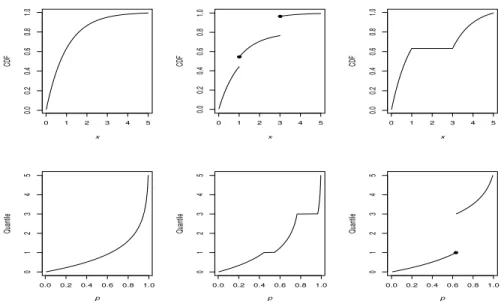
0 1 2 3 4 5 0.0 0.2 0.4 0.6 0.8 1.0 x CDF
0.0 0.2 0.4 0.6 0.8 1.0
0 1 2 3 4 5 p Quantile
0 1 2 3 4 5
0.0 0.2 0.4 0.6 0.8 1.0 x CDF
0.0 0.2 0.4 0.6 0.8 1.0
0 1 2 3 4 5 p Quantile
0 1 2 3 4 5
0.0 0.2 0.4 0.6 0.8 1.0 x CDF
0.0 0.2 0.4 0.6 0.8 1.0
0 1 2 3 4 5 p Quantile
Figure 1.1. CDFs and Quantile Functions
overloading the notation “·−1”) because, while a CDF may not be an invertible function, it is monotonic nondecreasing.
Notice that for the random variableX with CDFF, if
xπ=F−1(π), (1.13)
then xπ is theπquantile of X as defined in equation (1.6). Equation (1.13) is usually taken as the definition of theπquantile.
The quantile function, just as the CDF, fully determines a probability distribution.
Theorem 1.8 (properties of a quantile function)
If F−1 is a quantile function andF is the associated CDF,
1. F−1(F(x)) ≤x. 2. F(F−1(p))
≥p. 3. F−1(p)
≤x⇐⇒p≤F(x). 4. F−1(p
1)≤F−1(p2)ifp1≤p2.
5. lim↓0F−1(p−) =F−1(p).
(A quantile function is continuous from the left.)
6. If U is a random variable distributed uniformly over ]0,1[, then X = F−1(U)has CDF F.
The first five properties of a quantile function given in Theorem 1.8 char-acterize a quantile function, as stated in the following theorem.
Theorem 1.9
Let F be a CDF and letG be function such that
1. G(F(x))≤x, 2. F(G(p))≥p,
3. G(p)≤x⇐⇒p≤F(x), 4. G(p1)≤G(p2)ifp1≤p2, and
5. lim↓0G(p−) =G(p).
ThenGis the quantile function associated withF, that is, G=F−1.
Proof.Exercise. (The definitions of a CDF and a quantile function are suffi-cient.)
As we might expect, the quantile function has many applications that parallel those of the CDF. For example, we have an immediate corollary to Theorem1.7.
Corollary 1.7.1
IfF is a CDF andU ∼U(0,1), thenF−1(U)is a random variable with CDF F.
Corollary1.7.1is actually somewhat stronger than Theorem 1.7 because no modification is needed for discrete distributions. One of the most common applications of this fact is in random number generation, because the basic pseudorandom variable that we can simulate has a U(0,1) distribution.
The Probability Density Function: The Derivative of the CDF
Another function that may be very useful in describing a probability distribu-tion is the probability density funcdistribu-tion. This funcdistribu-tion also provides a basis for straightforward definitions of meaningful characteristics of the distribution.
Definition 1.16 (probability density function (PDF))
The derivative of a CDF (or, equivalently, of the probability measure) with respect to an appropriate measure, if it exists, is called theprobability density function,PDF.
The PDF is also called the density function.
Theorem 1.10 (properties of a PDF)
LetF be a CDF defined onIRd dominated by the measureν. Letf be the PDF defined as
f(x) =dF(x) dν .
Then over IRd
f(x)≥0 a.e. ν, (1.14)
f(x)<∞ a.e. ν, (1.15)
and Z
IRdfdν = 1. (1.16)
If XS is the support of the distribution, then
0< f(x)<∞ ∀x∈ XS.
Proof.Exercise.
A characteristic of some distributions that is easily defined in terms of the PDF is the mode.
Definition 1.17 (mode of a probability distribution)
Ifx0is a point in the supportXS of a distribution with PDFf such that
f(x0)≥f(x), ∀x∈ XS,
thenx0is called amodeof the distribution.
If the mode exists it may or may not be unique.
Dominating Measures
Although we use the term “PDF” and its synonyms for either discrete random variables and the counting measure or for absolutely continuous random vari-ables and Lebesgue measure, there are some differences in the interpretation of a PDF of a discrete random variable and a continuous random variable. In the case of a discrete random variableX, the value of the PDF at the pointxis the probability thatX =x; but this interpretation does not hold for a contin-uous random variable. For this reason, the PDF of a discrete random variable is often called a probability mass function, or just probability function. There are some concepts defined in terms of a PDF, such as self-information, that depend on the PDF being a probability, as it would be in the case of discrete random variables.