LifeCon1

(1)

Actuarial Mathematics Analytics

An open text authored by the Actuarial Community

(2)

(3)

Preface

Book Description

Actuarial Mathematics Analyticsis an interactive, online, freely available text.

• The online version contains many interactive objects (quizzes, computer demonstrations, interactive graphs, video, and the like) to promote deeper learning.

• A subset of the book is available foroffline reading in pdf and EPUB formats.

• The online text will be available in multiple languages to promote access to aworldwide audience.

What will success look like?

The online text will be freely available to a worldwide audience. The online version will contain many interactive objects (quizzes, computer demonstrations, interactive graphs, video, and the like) to promote deeper learning. Moreover, a subset of the book will be available in pdf format for low-cost printing. The online text will be available in multiple languages to promote access to a worldwide audience.

How will the text be used?

This book will be useful in actuarial curricula worldwide. It will cover the loss data learning objectives of the major actuarial organizations. Thus, it will be suitable for classroom use at universities as well as for use by independent learners seeking to pass professional actuarial examinations. Moreover, the text will also be useful for the continuing professional development of actuaries and other professionals in insurance and related financial risk management industries.

Why is this good for the profession?

An online text is a type of open educational resource (OER). One important benefit of an OER is that it equalizes access to knowledge, thus permitting a broader community to learn about the actuarial profession. Moreover, it has the capacity to engage viewers through active learning that deepens the learning process, producing analysts more capable of solid actuarial work. Why is this good for students and teachers and others involved in the learning process?

Cost is often cited as an important factor for students and teachers in textbook selection (see a recent post on the $400 textbook). Students will also appreciate the ability to “carry the book around” on their mobile devices.

(6)

Why loss data analytics?

Although the intent is that this type of resource will eventually permeate throughout the actuarial curriculum, one has to start somewhere. Given the dramatic changes in the way that actuaries treat data, loss data seems like a natural place to start. The idea behind the nameloss data analyticsis to integrate classical loss data models from applied probability with modern analytic tools. In particular, we seek to recognize that big data (including social media and usage based insurance) are here and high speed computation s readily available.

Project Goal

(7)

Chapter 1 Single Lifetime Distribution Essentials

1.1 The Lifetime Random Variable,

X

We begin by considering a non-negative random variable,X. Typically, we think ofX as the age at death of a newborn child. We summarize the distribution ofX using thedistribution function

F(x) = Pr(X ≤x) and thesurvival function

S(x) = 1−F(x) = Pr(X > x). Recall thedefining properties of a distribution function:

1. F(−∞) = limx→−∞F(x) = 0 2. F(∞) = limx→∞F(x) = 1 3. F(x)is nondecreasing inx.

Example - A Distribution due to Makeham (1860). This lifetime distribution provides a pleasant balance between complexity and practicality. It is more complex than simpler alternatives, such as the exponential distribution or a distribution due to Gompertz. Nonetheless, it can be (and is) used for selected actuarial applications.

One way to define the distribution is through the distribution function, given as

F(x) =

{

0 x <0

1−exp (−Ax−m(cx₋₁₎₎ _x_≥₀

Here, Aandmandc are parameters that the analyst may specify to approximate experience under consid-eration.

Both distribution and survival functions are bounded below by zero and above by one. Thus, we will not always write out the function over the entire domain, using these bounds to give implicit results. For examples, instead of writing out the function forx <0and forx≥0, we will write

S(x) = exp (−Ax−m(cx−1)).

We begin with the distribution and survival functions because they summarize the distribution for any random variable. To summarize the distribution for discrete random variables, use the probability mass function (pmf). For example, for a uniform distribution on the integers from 1 to 100, we have,

Pr(X=x) = 1

(8)

Figure 1.1: ??Timeline for Two Lives

To summarize the distribution for continuousrandom variables, use the probability density function (pdf), defined as

f(x) = ∂

∂xF(x) =F ′_(x).

For non-negative random variables, we also use the force of mortality (also known as the hazard rate or failure rate)

µ(x)≡ f(x) S(x) =

f(x) 1−F(x), to summarize the distribution.

Example - Makeham Distribution - continued. The probability density function can be calculated usingf(x) = ∂

∂xF(x). However, for this distribution the form is not intuitively appealing. Instead, we examine the force of mortality using the relation

µ(x) = ∂ ∂xF(x) 1−F(x)=−

∂ ∂xS(x)

S(x) =− ∂

∂xln(S(x)). For the Makeham distribution, we have

µ(x) =− ∂

∂xln(S(x)) =− ∂

∂x(−Ax−m(c x₋₁₎₎

=A+mcx(lnc) =A+Bcx, where B=mlnc.

Interpretation of the Force of Mortality. The force of mortality (fom) is the probability that a life agedxfails in a tiny interval, per unit of time. See the following calculations:

µ(x) = f(x)

1−F(x)= limϵ↓0

F(x+ϵ)−F(x)

ϵ 1−F(x) = lim

ϵ_↓0

Pr(x < X≤x+ϵ) ϵPr(X > x) = lim

ϵ↓0

(9)

1.2. THE FUTURE REMAINING LIFETIME,T 9

Figure 1.2: image

To relate the force of mortality to the survival function, we begin with the relation µ(x) = −_∂x∂ ln(S(x)). Integrating both sides, we have

S(y) = exp

{

−

∫ y

0

µ(x)dx

}

,

assumingS(0) = 1, orF(0) = 0. This gives us a method to recover the survival function using the force of mortality.

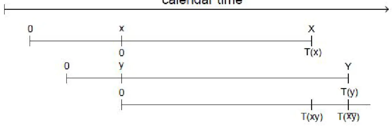
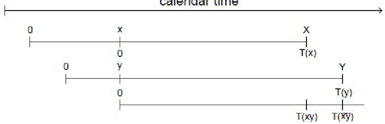
1.2 The Future Remaining Lifetime,

T

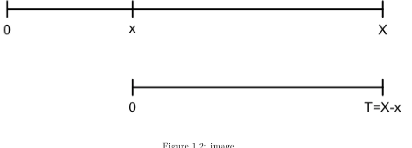
Recall that X is the age at death of an individual. Now we suppose that the individual survives to agex. Later, this will be the age at which the individual purchases an insurance contract. At agex, the individual’s future remaining lifetime is

T =T(x) =X−x.

1.2.1 Summarizing the Distribution of

T

To discuss the distribution ofT, we condition on the event{X≥x}={T ≥0}. Motivation, for individuals who do not survive to agex, they do not purchase an insurance contract and so are not under consideration here. Recall:

Conditional Probabilities. LetAandB be two generic events. Define the conditional probability

Pr(B|A) = Pr(AandB) Pr(A) .

Example - Uniform Distribution - continued. Suppose that X ∼U(0,100) and that x= 30. The distribution function ofT =T(30) =X−30is

Fx(t) = Pr(T ≤t) = Pr(X−30≤t|X ≥30) =

Pr(30≤X≤30 +t) Pr(X ≥30)

=

30+t−30 100

1− 30 100

= t

70 ⇒T ∼U(0,70).

(10)

In general, the distribution function ofT is

Fx(t) = Pr(T ≤t) = Pr(T≤t|T ≥0) = Pr(X≤x+t|X ≥x) =

Pr(x < X≤x+t) Pr(X ≥x) =F(x+t)−F(x)

1−F(x) = 1−

S(x+t) S(x) .

That is, the distribution functionFx(·)is a conditional distribution function in terms of the random variable X, where one conditions on survival to agex.

Similarly, the survival function ofT is

Sx(t) = 1−Fx(t) = Pr(T > t|T ≥0) =

S(x+t) S(x) .

1.2.2 Actuarial Notation

We write the distribution function as

tqx=Fx(t),

and interpret this to mean “the probability a life aged(x)will die withint years”. We write the survival function as

tpx=Sx(t) = 1−Fx(t) = 1− tqx and interpret this to mean “the probability a life aged(x)will survive tyears”. The probability density function of T is

∂

∂tFx(t) = ∂ ∂t

(

1−S(x+t) S(x)

)

=−S ′_(x₊_t) S(x+t)

S(x+t) S(x)

= µx+t tpx

The force of mortality ofT is

p.d.f. s.f. =

tpxµx+t tpx

=µx+t This is the force of mortality ofxat timet, corresponding to agex+t.

Note that this the same as force of mortality for the random variableX but evaluated at timet, corresponding to agex+t.

Example - Uniform Distribution - Summary. Suppose that X ∼U(0, ω). The (unconditional) distri-bution and survivor functions ofX are:

F(x) =

{ _x

ω 0≤x≤ω 1 0> ω S(x) = 1−x

ω = ω−x

ω .

The survivor and distribution functions ofT (conditional on survivorship to agex) are:

tpx=

S(x+ 1) S(x) =

ω₋(x+1)

ω ω₋x

ω

= 1− t ω−x 0≤t≤ω−x uniform(0,ω−x)

tqx=

(11)

1.2. THE FUTURE REMAINING LIFETIME,T 11

The force of mortality is

µx=

f(x) 1−F(x) =

1

ω 1−_ωx =

1 ω−x.

Example - Makeham Distribution - Summary. Suppose that X has a Makeham distribution with parametersA,mandc. Recall that the survival function of X is

S(x) = exp (−Ax−m(cx−1)). and the force of mortality isµ(x) =A+Bcx_{, where} _B₌_m_ln_c. The survival function ofT (conditional on survivorship to agex) is

tpx=

S(x+t) S(x) =

exp (−A(x+t)−m(cx+t₋₁₎₎ exp (−Ax−m(cx−₁₎₎ = exp(−At−mcx(ct−1)).

Note that you can think of this conditional survival function as having the same form as the original Makeham survival distribution with the parametermreplaced bymcx_.

1.2.3 Successive Conditioning

From the definition of the conditional survival function, we may write

S(x+t) =S(x)×Sx(t).

On the left-hand side, this is the probability that a person age (0) survivesx+tyears. On the right-hand side, the first term is the probability that a person age (0) survives xyears. The second term is the probability that a person age (x) survives an additionaltyears. In actuarial notation, we may express this as

x+tp0= xp0× tpx. An immediate extension of this idea is

r+tpx= rpx× tpx+r. To check this, simply write down the definition of each actuarial symbol

Sx(r+t) =Sx(r)×Sx+r(t) which is

S(x+r+t) S(x) =

S(x+t) S(x) ×

S(x+r+t) S(x+t) that immediately establishes the relationship.

We interpret the relation $~_{r+t} p_x = ~_r p_x ~t p{x+r} $ to mean that “the probability that a person age (x) survives an additionalr+tyears” equals “the probability that a person age (x) survives an additionalryears” times “the probability that a person age (x+r) survives an additionalt years.”

Note that the choices of t, r,andxdepend on the problem. For example, you may wish to evaluate 15p30

as 5p30 10p35 or as 10p30 5p40, depending on the problem. Further, in some applications, it is useful to the

use the successive conditioning recursively. For example, we might write

(12)

Figure 1.3: image

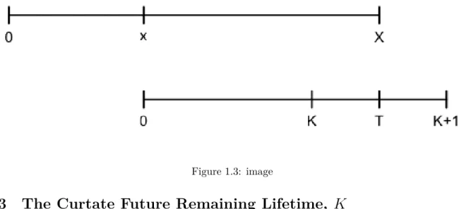
1.3 The Curtate Future Remaining Lifetime,

K

Define K =K(x) = greatest integer ≤T, sometimes denoted as int(T) or [T]. This is called thecurtate future remaining lifetime. It is a discrete random variable and so we can discuss the probability mass function

Pr(K=k) = Pr(k≤T < k+ 1) = kpx− k+1px = kpxqx+k = k|qx In this expression, we used successive conditioning to write k+1px= kpxpx+k .

Important. Note that we are still calculating the distribution function conditional on survivorship to agex. We could emphasize by writing Pr(K=k|K≥0) = Pr(k≤T < k+ 1|T ≥0).

Read the notation k|qx to mean “ the probability a life aged xdies within one year, deferred by kyears”. So, we define theactuarial notation

k|nqx= Pr(x+k≤T < x+k+n|T >0) = S(x+k)−S(x+k+n)

S(x) = kpx nqx+k

(13)

Chapter 2 Classic Joint Life Fundamentals

2.1 Joint Life Fundamentals

We consider two lives who are agesxandy, respectively, at contract initiation. The future remaining lifetimes areT(x)andT(y)at contract initiation. To aid with interpretation, we think of “x” has the “insured’s” and “y” as the “spouse’s” age because many joint life contracts are sold to married couples (although the theory

clearly applies to many other situations of interest, e.g., an insured with a grandchild).

We are interested in known functions of these future remaining lifetimes (e.g., “g”), g(T(x), T(y)); these functions are known as astatus. Here are the two most important examples:

Joint Life Status. In this case, the interest is ing(T(x), T(y)) = min(T(x), T(y)) = T(xy), which is the time until the first of the two lives fails.

Last Survivor Status. In this case, the interest is in g(T(x), T(y)) = max(T(x), T(y)) =T(xy), which is the time until the second of the two lives fails.

To warm up, start by assuming thatT(x)andT(y)are independent.

Figure 2.1: image

(14)

2.1.1 Joint-Life Probability Functions

The distribution function ofT =T(xy)is

FT(t) = Pr(T(xy)≤t) = Pr(min(T(x), T(y))≤t) = 1−Pr(min(T(x), T(y))> t) = 1−Pr(T(x)> t) Pr(T(y)> t) = 1− tpx× tpy. We write the survivor function as

tpxy= 1−FT(t) = tpx× tpy. From this, the density function is

fT(t) = FT′(t) =− ∂

∂t(tpx× tpy) = −

(

tpx ∂

∂t tpy+ tpy ∂ ∂t tpx

)

= tpx(tpyµy+t) + tpy(tpxµx+t) = tpx tpy(µx+t+µy+t). Thus, the force of mortality is

µxy(t) =

fT(t) 1−FT(t)

=µx+t+µy+t.

2.1.2 Last-Survivor Probability Functions

The distribution function is

FT(t) = Pr(T(xy)≤t) = Pr(max(T(x), T(y))≤t) = Pr(T(x)≤t, T(y)≤t) =IN D Pr(T(x)≤t) Pr(T(y)≤t) = tqx tqx= (1− tpx)×(1− tpy). We write the survivor function as

tpxy= 1−FT(t) = tpx+ tpy− tpx tpy. From this, the density function is

fT(t) = FT′(t) =− ∂

∂t(tpx+ tpy− tpx tpy) = tpxµx+t+ tpyµy+t− tpx tpy(µx+t+µy+t) = tpxµx+t tqy+ tpyµy+t tqx. Thus, the force of mortalityµxy(t) =

fT(t)

1−FT(t) does not have a straightforward expression.

2.1.3 Examples

1. Suppose that T(x) is uniformly distributed (DeMoivre) over (0, wx−x), T(y) is uniformly distributed over(0, wy−y), and thatT(x)andT(y)are independent. Letwx= 100, x= 30,wy= 110, andy= 28. Determine: a) 20p30:28 b)µ30:28(20)c) 20p_30:28

Solution.

a) ForT(x)∼U(0, wx−x)(DeMoivre), recall that

tpx= 1− t wx−x

, tpxµx+t= 1 wx−x

, andµx+t= 1 wx−x−t

(15)

2.1. JOINT LIFE FUNDAMENTALS 15

Thus,

20p30:28= 20pm30 20p

f

28=

(

1− 20 100−30

) (

1− 20 110−28

)

= 0.54.

b)

µ30:28(20) =µm30+20+µ28+20(20)f =

1 100−50+

1

110−48 = 0.0361 c)

20p_30:28= 20pm30+ 20pf28− 20p30:28

= 50 70 +

62

82−0.54 = 0.930

2. Suppose that T(x) is exponentially distributed with force of mortalityµx(t) =µ1 = 0.02, T(y)is

expo-nentially distributed with force of mortalityµy(t) =µ2= 0.015, and thatT(x)andT(y)are independent.

Provide expressions for: a) tpxy b)µxy(t)c) tpxy Solution.

a) ForT(x)is exponentially distributed with force of mortalityµx(t) =µ1, recall that

tpx= exp(−µ1t).

Thus,

tpxy= tpx× tpy= exp(−µ1t) exp(−µ2t) = exp(−(0.02 + 0.15)t) = exp(−0.035t).

b)

µxy(t) =µx(t)m+µy(t)f =µ1+µ2= 0.035.

c)

tpxy= tpx+ tpy− tpx tpy = exp(−µ1t) + exp(−µ2t)−exp(−(µ1+µ2)t)

= exp(−0.02t) + exp(−0.015t)−exp(−0.035t).

3. Recall that we can express the Gompertz force of mortality asµx =Bcx. In this case, we may express the survival function as S(x) = exp(−m(cx₋_{1)), where}_m₌_B/_ln_c_{and the conditional survivor function} forT(x)as

tpx= exp(−m(cx+t−cx)) = exp(−mcx(ct−1)).

Assume that the Gompertz force governs mortality for males and females (with a common parameters m andc).

Determine the value ofw so that we may write tpxy= tpw. That is, show that we can compute joint life probabilities using a single life table for the Gompertz case.

Solution.

The joint life survival probability is

tpxy = tpx× tpy

= exp(−mcx(ct−1)) exp(−mcy(ct−1)) = exp(−(cx+cy)×m(ct−1)) So, definewto be the solution ofcw=cx+cy. With this, we may write

(16)

2.1.4 Relating Status Distributions

It is possible to relate the joint life and last-survivor status without the assumption of independence. Consider the eventsA={T(x)≤t}andB ={T(y)≤t}. Now,

AandB= {T(x)≤t, T(y)≤t}={T(xy)≤t} and

AorB = {T(xy)≤t}. BecausePr(AorB) = Pr(A) + Pr(B)−Pr(AandB), we have

Pr(T(xy)≤t) = Pr(T(x)≤t) + Pr(T(y)≤t)−Pr(T(xy)≤t) so that

tpxy= tpx+ tpy− tpxy.

Note that this relationship holds without using the assumption of independence between lives.

2.1.5 Lifetime Moments

For the expected survivor time of the joint life status, we have

˙

exy=E T(xy) =

∫ _∞

0

tfT(xy)(t)dt=

∫ _∞

0

(1−FT(xy)(t))dt

=

∫ _∞

0

tpxydt.

The third equality comes from an integration by parts. Similarly, for the expected last-survivor time,

˙

exy = E T(xy) =

∫ _∞

0

tpxy dt

=

∫ _∞

0

(tpx+ tpy− tpxy)dt = e˙x+ ˙ey−e˙xy.

Note that this relation holds without regard to the independence between lives assumption.

Special Case - Exponential Distribution. Suppose thatT(x)is exponentially distributed with force of mortalityµx(t) = µ1, T(y) is exponentially distributed with force of mortalityµy(t) =µ2, and that T(x)

andT(y)are independent. Then, forx, we have tpx= exp(−µ1t)and

˙

ex= E T(x) =

∫ _∞

0

tpx dt= 1 µ1

Similarly, for the joint-life status, we have tpxy= tpxy× tpxy= exp(−(µ1+µ2)t)which is an exponential

distribution with force of mortalityµ1+µ2. This yieldse˙xy= 1/(µ1+µ2).

Now, for the last-survivor status, we have

1− tpxy= FT(xy)(t) = Pr (max(T(x), T(y))≤t)

(17)

2.1. JOINT LIFE FUNDAMENTALS 17

and

˙

exy= e˙x+ ˙ey−e˙xy = 1

µ1

+ 1 µ2 −

1 µ1+µ2

.

Example - Exponential Distribution. Suppose in addition thatµ1= 0.02andµ2= 0.015. Then,

˙ ex=

1 µ1

= 50, e˙y = 1 µ2

= 66.67, e˙xy= 1 µ1+µ2

= 28.57.

Further,

˙

exy= e˙x+ ˙ey−e˙xy = 50 + 66.67−28.57 = 88.1.

Moreover, we have

Cov(T(xy), T(xy)) = E {T(xy)×T(xy)} −ET(xy)×E T(xy) = E {max(T(x), T(y))×min(T(x), T(y))} −e˙xy×e˙xy = E {T(x)×T(y)} −e˙xy×e˙xy = e˙xe˙y−e˙xy×e˙xy= 50×66.67−88.1×28.57 = 816.48.

Exercise. Consider a population containing smokers (s) and non-smokers (ns) where their forces of mortality are related as

µnsx = 1 2µ

s x.

For the non-smoking population, mortality is given aslx= 75−x,x≥0. Consider two lives, a non-smoker age 65 and a smoker age 55, and assume lives are independent. Calculatee˙65:55.

Solution.

For non-smokers, the force of mortality is µnsx = −d ldxx

1

lx =

1

75−x. Thus, the conditional survival force is tpnsx = 1−

t

75₋x.

For smokers, the force of mortality isµs

x=752−x so that the conditional survival force is

tpsx= exp

(

−

∫ t

0

µs_x₊_rdr

) = exp ( −2 ∫ t 0 1

75−x−r dr

)

= exp(2 ln (75−x−r)|t0

)

= exp

(

2 ln75−x−t 75−x

)

=

(

1− t 75−x

)2

Thus,

tp65:55= tpns65 tps55=

(

1− t 10

) (

1− t 20

)2

and

˙ e65:55=

∫ 10

0

tp65:55dt

=

∫ 10

0

(

1− t 10

) (

1− t 20

)2

(18)

As follow-ups, note that 1) e˙ns₆₅ = 5(= 75−₂65). 2)e˙s

55=

∫20 0

(

1−₂₀t)2dt= 20₃. 3)

˙

e_65:55= 5 + 20

3 −3.54 = 8.12

̸

=

∫ 10

0

tp65:55 dt.

2.2 Joint Life and Last-Survivor Annuities and Insurances

2.2.1 Continuous Case

We are now in a position to express the expected present value (EPV) of several annuity and insurance contracts using traditional notation. It is convenient to begin with the continuous case when we know the exact moment of payment. You will see that the treatment is completely analogous to the single life case -thus, we will be brief in our presentation of different variations.

To begin, a joint life insurance is a life insurance which pays a benefit of 1 immediately upon the first to die ofxandy. It is also known as afirst to die insurance. In this case, the random present value of future benefits isvT(xy)_{= exp(}₋_δT_(xy))_{which has expected present value}

¯ Axy=

∫ _∞

0

e−δt tpx tpx(µx+t+µy+t) dt.

Similarly, the EPV of last-survivor insurance, with pays a benefit of 1 immediately upon the second death, is

¯ Axy=

∫ _∞

0

e−δt(tqy tpxµx+t+ tqx tpyµy+t) dt.

As can be seen from the expressions, the integrals can be a little annoying to compute. Thus, it is often easier to work with the corresponding annuities and then use the relationship between insurances and annuities to evaluate the insurance quantities.

To this end, define a joint life annuityto be an annuity payable until the first death of xand y. That is, there is a continuous payment at the rate of 1 per year while both are alive. In this case, the EPV is

¯ axy=

∫ _∞

0

e−δt tpxy dt.

The random variable underpinning the joint life annuity isa¯_T₍_xy₎_|= 1−exp(−_δδT(xy)). So, as with single life functions, we have

joint life annuity rv=1−joint life insurance rv δ

Taking expectations of each side yields

¯ axy=

(19)

2.2. JOINT LIFE AND LAST-SURVIVOR ANNUITIES AND INSURANCES 19

Similarly, alast survivor annuityis an annuity payable where there is a continuous payment at the rate of 1 per year while at least one ofxandy is alive. In this case, the EPV is

¯

axy= ¯ax+ ¯ay−¯axy and can be related to last-survivor insurance through the expression

¯ axy=

1−A¯xy δ .

As we will see in subsequent exercises and modules, temporary and deferred annuities, as well as term, endowment and deferred insurances, can be defined in a fashion similar to single life functions.

Special Case: Premiums For Dependent Lives. Consider a fully continuous life insurance forxandy. Suppose that

1) premiums are payable until the first death 2) a benefit of 1 is payable at the second death.

The joint mortality for T(x)andT(y)is not independent but given by

tpxy=rtpx+ (1−r)tpx tpy.

For simplicity, assume that the mortality forT(x)andT(y)follow a common exponential distribution,

tpx=e−µt= tpy. Show that the annual premium is µ(2µ+δ)

δ+(1+r)µ. Solution

The premiumP is the solution of_A¯_xy ₌_P_¯_a_xy_{. Now}

¯ axy=

∫ _∞

0

e−δt tpxy dt

=

∫ _∞

0

e−δt(r tpx+ (1−r)tpx tpy) dt

=

∫ _∞

0

e−δt(re−µt+ (1−r)e−2µt) dt

= r

µ+δ + 1−r 2µ+δ =

δ+ (1 +r)µ (µ+δ)(2µ+δ) Further

¯ Ax=

∫ _∞

0

e−δt tpxyµx+tdt

= µ

∫ _∞

0

e−δte−µt dt= µ

µ+δ = ¯Ay and

¯

Axy= ¯Ax+ ¯Ay−A¯xy= 2 µ

µ+δ −(1−δ¯axy). Thus

P= ¯ Axy

¯ axy

= 2 µ µ+δ −1

¯ axy

−δ

(20)

2.2.2 Discrete Case

Start with a generic time until failureT that may be a function of one or more lives. Define the curtate time until failureK= [T], where[·]denotes the greatest integer function. Then,

Pr(K=k) = Pr(k≤T < k+ 1) =FT(k+ 1)−FT(k).

Special Case. Joint Life Status. In this caseT =T(xy), and soKmay be denoted asK(xy) = [T(xy)]. We may also think of the curtate random variable asK(xy) = min(K(x), K(y)).

This has probability mass function

Pr(K=k) = k+1qxy− kqxy= kpxy− k+1pxy = kpxyqx+k:y+k≡ k|qxy.

For insurances, we have the “first-to-die” insurance

Axy= EvK(xy)+1= ∞

∑

k=0

vk+1 k|qxy.

This is the EPV for a payment of 1 at the end of the year of the first death among (x) and (y). For annuities, we have

¨

axy= E ¨a_K₍_xy₎₊₁_|= ∞

∑

k=0

vk kpxy.

This is the EPV for a payment of 1 at the beginning of each year while both (x) and (y) are alive.

Special Case: Recursive Calculation for Discrete Joint Life Annuities. For a joint life annuity on livesxandy with payments of 1 per year in advance, the EPV can be written recursively as:

¨

axy= 1 +vpxy¨ax+1:y+1.

Check: The EPV is

¨ axy=

∞

∑

k=0

vk kpxy.

By successive conditioning, we may write

k+1pxy=pxy kpx+1:y+1.

Thus, using k=j+ 1, we have

¨

axy= 1 + ∞

∑

k=1

vk kpxy= 1 + ∞

∑

j=0

vj+1 j+1pxy

= 1 +vpxy ∞

∑

j=0

vj jpx+1:y+1= 1 +vpxy¨ax+1:y+1.

(21)

2.2. JOINT LIFE AND LAST-SURVIVOR ANNUITIES AND INSURANCES 21

2.2.3 Generic Statuses

As with single life functions, one can readily extend fundamental principles to handle many practical contracts. We indicate how to do so in the discrete, with similar extensions to the continuous case analogous

We will consider a generic status “u”.

Varying Benefits and Payments. LetK be the curtate failure time associated with that status. For an insurance benefit the paysbK+1 for failure in theKthperiod, the EPV is

∞

∑

k=0

bk+1vk+1 k|qu.

For an annuity benefit that paysπhat the beginning of each year when the statusuhas survived, the EPV is

E

(_K ∑

h=0

πhvh

)

= ∞

∑

k=0

πkvk kpu.

Generic Status - Insurance and Annuities. Temporary and deferred annuities, as well as endowment and deferred insurances, can be defined in a fashion similar to single life functions.

Consider two lives,xandybut letT(y) =nwith probability one. Then, for the joint life status, we have ¨

axy= ¨a_x_:_n_| and

Axy=A_x_:_n_| Similarly for the last-survivor status,

¨ axy= ¨a

x:n_|= äx+ ¨an|−äx:n|= ¨an|+ n|äx

an annuity that is payable for certain fornyears and as long as (x) survives thereafter.

Generic Status - Multiple Lives. We can allow multiples lives on a contract, say, x, y, and z, in the same fashion. For example, compute the survival function

tpxyz = tpx× tpy× tpz assuming independence among lives.

Further, we can one life, say z, but let T(z) =n with probability one. Then, for example, the joint life annuity on the triple becomes

¨

axyz= ¨a_xy_:_n_|

a temporary joint life annuity on the joint statusxy. In this way, we can introduce temporary and deferred annuities, as well as endowment and deferred insurances, for the joint life status and last-survivor status.

To summarize, here are some examples of different statuses we regularly consider: cl|cl Status (u) & Description & Status (u) & Description

(22)

xy& last-survivor & 1

x:n_| & contingent xyz & joint lives & 1

xy & contingent xy:n|& temporary &x|y & reversionary ## Common Shock Model for Dependent Lives

Suppose that T∗(x) and T∗(y) are unobserved future lifetimes for x and y that are independent of one another. Let Z be a lifetime random variable that is common to both xand y for e.g., disasters such as earthquakes and hurricanes. TakeT∗(x),T∗(y),Z to be mutually independent.

LetT(x) = min(T∗(x), Z)andT(y) = min(T∗(y), Z)be the observed future lifetimes forxandy. Note that they are not independent because they share the common shock random variableZ.

For convenience, assume that the distribution ofZ is exponential with constant forceλ. Now, the survival function forxis

tpx= Pr(T(x)> t) = Pr(min(T∗(x), Z)> t) = Pr(T∗(x)> t) Pr(Z > t) = tp∗xe− λt

Similarly, tpy = tp∗ye−λt. The joint survival probability is

tpxy= Pr(min(T(x), T(y))> t) = Pr(min(T∗(x), T∗(y), Z)> t) = Pr(T∗(x)> t) Pr(T∗(y)> t) Pr(Z > t) = tp∗x tp∗ye−

λt

= tpx tpyeλt.

From this, we can also calculate the joint force of mortality

µxy(t) =− ∂

∂t ln tpxy == −∂

∂t

(

ln tpx+ ln tpy+ lneλt

)

=µx(t) +µy(t)−λ.

Example. You have calculated the expected present value of a last survivor life insurance of 1 onxandy. You assumed:

The death benefit is payable immediately on the second death.

The future lifetimes ofxandyare independent, and each life has a constant force of mortality withµ= 0.06. Assume δ= 0.05.

Your supervisor points out that these are not independent future lifetimes. Each mortality assumption is correct, but each includes a common shock component with constant force 0.02.

Calculate the increase in the expected present value over what you originally calculated. Solution.

We wish to calculate _A¯CS xy −A¯

IN D

xy . Under the independence model, we have

¯ Ax=

∫ _∞

0

e−δt tpxµx+tdt=

∫ _∞

0

e−δte−µtµdt= µ µ+δ. Thus,

¯ Ax=

0.06 0.06 + 0.05 =

6 11 = ¯Ay. Further,

¯ Axy=

∫ _∞

0

e−δt tpxyµxy(t)dt=

∫ _∞

0

(23)

2.3. ADDITIONAL EXAMPLES AND APPLICATIONS 23

so that_A¯_xy₌ 0.12 0.17 =

12 17 and

¯

AIN D_xy = ¯Ax+ ¯Ay−A¯xy= 2 6 11−

12

17= 0.385.

For the common shock model, the original force of mortality was 0.06, so the new force of mortality is 0.04. Thus,

¯ Ax=

∫ _∞

0

e−δt tpxµx+tdt=

∫ _∞

0

e−0.05te−0.04te−0.02tµdt= 6 11,

as before. The same is true for_A¯_y_{. The joint force of mortality is}_µ_xy_{(t) = 0.06 + 0.06}₋_{0.02 = 0.10. Thus,} the joint survival function is tpxy=e−0.10t. This yields

¯

ACS_xy = µxy µxy+δ

= 0.10 0.10 + 0.05 =

2 3, and

¯

ACS_xy = ¯Ax+ ¯Ay−A¯CSxy = 2 6 11−

2

3 = 0.42423. Thus, the increase is

¯

ACS_xy −A¯IN D_xy = 0.42423−0.385 = 0.0392.

2.3 Additional Examples and Applications

2.3.1 First To Die with Mortality Adjustments

The traditional “first to die” insurance pays 1 at the end of the year of death of either (x) or (y). The expected present value of this insurance is

Axy= ∞

∑

k=0

vk+1 kpxyqx+k:y+k

where kpxy is the probability that both (x) and (y) survivek years andqx+k:y+k is the probability that at least one of (x+k) and (y+k) dies within the year. To evaluate this, it is customary to begin by assuming independent lives, so that

AIN D_xy = ∞

∑

k=0

vk+1 kpx kpy(1−px+k×py+k).

From the formula forAIN D

xy , it is easy to see that as interest increases, the expected present value decreases. What about mortality? Let us think of (x) as a male life and (y) as a female life. Consider a mortality adjustment to male lives of the form

qrevised_x = (1−c)×q_xbase.

This is a coarse adjustment but will give us a flavor as to what happens to insurance prices as mortality increases or decreases. Viewers should verify thatAIN D_xy increases as the adjustment coefficientc decreases. (Although a separate exercise, atc≈0.35, male mortality is roughly equivalent to female mortality for our

Indonesian data.)

The dynamic graph shows values ofAIN D

(24)

2.3.2 Reduction Factors for Joint and Surviving Annuities

At retirement from employment, it is common for pension plan participants to have earned a lifetime annuity in the amount ofP EN per year whose expected present value isP ENäx. Suppose that the participant has a spouse (or other dependent) age (y) and wishes to purchase an annuity that continues to provide benefits even after (x) has died to the survivor (y). For example, a joint and 75% survivor annuity makes an annual payment of 1 while both (x) and (y) are alive, a payment of 0.75 while only one of (x) and (y) are alive, and no payments following the death of both (x) and (y). Thus, expected present value of this annuity is 0.75(äx+ äy)−0.50¨axy. To equate these values, we would require the new pension amount P ENJ S to be that amount so that P ENa¨x = P ENJ S(0.75×(äx+ äy)−0.50¨axy). More generally, define the annuity factor

AN N F ACT OR= ¨ax

RED(¨ax+ ¨ay) + (1−2RED)¨axy , for the reduction factorRED.

The dynamic graph shows values of AN N F ACT OR plotted against the reduction factor RED and age, where for plotting purposes we use a common age x=y. The graph shows the dynamic effect over interest rateiranging from 0 to 20%. The graph shows that it is difficult to provide a general interpretation for the reduction percentage and age. However, as the interest rate i increases, the factor approaches one for all values of the reduction percentage and age.

2.3.3 Dependent Joint Life Annuities with Common Shock

Using the common shock model, we can relate the joint survival probabilities to the marginal survival probabilities through the expression

kpxy=eλk kpx kpy. With this, we may express the dependent joint life annuity as

¨ aDEP_xy =

∞

∑

k=0

e−δk kpxy= ∞

∑

k=0

e−δkeλk kpx kpy

= ¨aIN D_xy @(δ−λ).

Here, ¨aIN D_xy @(δ−λ)is joint life annuity calculated assuming (x) and (y) are independent lives at a revised force of interestδ−λ.

(25)

Chapter 3 Policy Values

3.1 Special Case: Whole Life Insurance Policy

We can illustrate many important concepts in terms of this basic policy. For concreteness, we assume the fully continuous case, that pays 1 immediately upon the failure of the policyholder and where level premiums are payable continuously throughout the year until the moment of failure.

As before, we assume that contract initiation age is x. We now wish to establish the value of the policy t years later when the policyholder is agex+t(if alive).

At (policy) time t, we define the future (net) loss variable (to the insurer) to be the excess of the present value of future insurance benefits (PVFB) over the present value of future net premiums (PVFNP)

Ln_t =P V F B−P V F N P =vT−t−Pn¯a_T₋_t_|. BecauseT is random,Ln

t is a random variable; although we focus on its mean, the variance and distribution function are also important for different applications.

To get a step closer to reality, we can easily add expenses into the mix. As before, we think of a “gross premium,”GorPG_{, as an income that accounts for benefits and expenses. With this, define the}_{future gross} loss variableto be

Lgt =P V F B+P V F E−P V F GP,

where PFVE represents the present value of future expenses and PVFGP represents the present value of future gross premiums.

Thepolicy value, also known as the reserve, is the expected future loss variable, typically denoted asV = EL. Sometimes we write tV = E (Lt|T > t) to emphasize the conditional expectation, that is, we are only computing policy values for individuals who have survived t future years. In this basic case, the constant premium rateP is determined at contract initiation, e.g., att= 0.

Policy Value. Specifically, at time t, the EPV of future benefits isE (vT−t|T > t) = ¯Ax+t. The EPV of future premiums isE (Pn¯a_T₋_t_||T > t) =Pn¯ax+t. With these, the net premium policy value is

tVn = ¯Ax+t−Pn¯ax+t.

In the premium module, we learned that we could derive net premiums through the equivalence principle, that is, findPn _{such that}_E_Ln

0 = 0Vn = 0. Thus, we havePn= ¯Ax/¯ax.

Variance. With the net premium and the relation ¯a_T₋_t_| = (1−vT−t_{)/δ, we write the net premium loss} variable as

Ln_t =vT−t−Pn1−v T₋t

δ =

(

1 +P δ

)

(26)

birth

contract

initiation

death

Lifetime

0 x

x+t

X

Contract

Time

contract

valuation

0 t

T

Figure 3.1: image

Thus, we have

Var(Ln

t|T > t) =

(

1 + P δ

)2

Var(vT−t_|_{T > t)}

=

(

1 + P δ

)2₍ 2_A_¯

x+t−A¯2x+t

)

.

Here, recall the notation 2_A_¯_{means compute the EPV of a whole life insurance at force of interest}_2δ. Example. Suppose that mortality follows De Moivre’s law with limiting age w = 100. Let i = 6% and x= 35. Then,

¯ A35=

∫ 65

0

vttp35µ35+t dt= 1 65

∫ 65

0

vtdt= 1 65a¯65|

and

Pn=A¯35 ¯ a35

= δA¯35 1−A¯35

= δ¯a65|/65

1−¯a₆₅_|/65 = 0.020266. Similarly, we have_A¯₃₅₊_t_{= ¯}_a

65−t|/(65−t)and

¯ a35+t=

1−A¯35+t

δ =

1−¯a₆₅₋_t_|/(65−t) δ

The policy value may be written as

tVn= ¯ a₆₅₋_t_|

65−t−(0.020266)

(27)

3.1. SPECIAL CASE: WHOLE LIFE INSURANCE POLICY 27

0

10

20

30

40

50

60

0.0

0.2

0.4

0.6

0.8

1.0 time

P

olicy V

alue

standard deviation

policy value

Figure 3.2: image

and its associated variability is

Var(Ln

t|T > t) =

(

1 +0.020266 δ

)2( 2_¯_a 65−t| 65−t −

[_¯_a

65−t| 65−t

]2)

= 1.813821

( ₂

¯ a₆₅₋_t_| 65−t −

[_¯_a

65−t| 65−t

]2)

using δ = ln(1.06). Figure 1 summarizes these calculations. Note that the policy value is 0 att = 0. At t= 65, the policy value becomes 1. Also att= 65, there is no uncertainty about the value of the policy and so the standard deviation becomes 0.

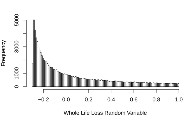
Simulation. With Monte Carlo, or stochastic, simulation, we can easily get additional insights. To illustrate ideas, we focus on the loss random variable att= 10.

We letU be a randomly generated uniform random number on(0,1). In this case, the future (givenT >10) remaining lifetime random variableT−10 = 55∗U, that is, uniform on the interval(0,55). For this randomly generated future lifetime, the corresponding loss random variable is

Lnt =vT−10−(0.020266)¯aT−10|.

(28)

Whole Life Loss Random Variable

Frequency

−0.2

0.0

0.2

0.4

0.6

0.8

1.0

0 1000

3000

5000

Figure 3.3: image

turned out to be 0.055512; this is very close to the theoretically correct value determined above, 0.055701. The standard deviation from the Figure 2 sample is 0.3459959, close to 0.3466074 that was determined by theory. Figure 2 shows that the maximum value is 1.0 (corresponding toT = 10) and the minimum value is -0.29310, corresponding toT = 65.

The simulation gives a quick method to calculate the same values that we could determine from theory. Simulation also allows us to readily see the entiredistribution of the loss random variable - for this simple example, we could determine the distribution from theory. Moreover, theoretical calculations allow us to readily visualize patterns over evolving time durationt. As we will see, the advantage of simulation methods is that they provide flexibility to easily modify design aspects such as timing of benefits and payments, as well as for discounting mechanisms such as variable interest rates. You will find it helpful to become facile in doing calculations using both theory and simulation approaches.

Try an animated display where the distribution changes by the policy duration

Exercise. Show that the probability density function for the loss random variable is

fLt(y) =

1

(65−t)(yδ+Pn₎. Solution.

The distribution function ofLnt is

FLt(y) = Pr(L

n

t ≤y) = Pr(v

T−t₋_P

(

1−vT−t δ

)

≤y)

= Pr(vT−t≤yδ+P

δ+P ) = Pr(T−t≥ − 1 δln

(

yδ+P δ+P

)

(29)

3.2. EXERCISE: FULLY CONTINUOUSNYEAR ENDOWMENT POLICY 29

Conditional onT > t,T −t is uniform on(0,65−t), so

FLt(y) =

65−t−1_δln

(

yδ+P δ+P

)

65−t Taking a partial derivative with respect toy yields

fLt(y) =

∂ ∂y

65−t−1

δln

(

yδ+P δ+P

)

65−t = −1

δ(65−t) ∂

∂yln(yδ+P)

= 1

(65−t)(yδ+P), as required.

3.2 Exercise: Fully Continuous

n

Year Endowment Policy

In this policy, a benefit of 1 is payable immediately upon failure. Premiums are payable at a constant annual rate ofP per year that is determined at contract initiation by the equivalence principle. Assume a constant force of interest and no expenses. The policy valuation is at timet < n.

1. Express the (net) premium using standard actuarial notation.

2. Express the loss random variable using standard interest theory symbols. 3. Express the policy value using standard actuarial notation.

4. Express the standard deviation of the loss random variable using standard actuarial notation.

5. Suppose that x= 35, n = 20, i = 6%, t = 5, and mortality follows deMoivre’s law with limiting age w= 100. Calculate the policy value and standard deviation.

Solution.

1. The net premium isP = A¯x:n|

¯

a_x_:_n_|.

2. IfT < t, then the policy is complete and we do not consider it further. IfT ≥n(exceeding the endowment period), then the loss random variable isLt=vn−t−Pa¯n₋t_|, where P is from part (1). Ift≤T < n, then the loss random variable isLt=vT−t−Pa¯_T₋_t_|. We summarize this as

Lt=

{ _vT−t₋_P_a_¯

T−t| t≤T < n vn−t−Pa¯_n₋_t_| T ≥n

3. Recall that the “n−t” single premium endowment issued to a life agex+thas loss

LInsurancet =

{

vT−t _{T < n} vn−t _T_≥_n and expectation_A¯

x+t:n−t|. Similarly, an “n−t” temporary life annuity issued to a life agex+thas loss

LAnnuity_t =

{

¯

a_T₋_t_| T < n ¯

a_n₋_t_| T ≥n

and expectation¯a_x₊_t_:_n₋_t_|. Thus, the loss random variable is justLt=LInsurancet −P L Annuity

(30)

4. Using the relationa¯n_|= (1−vn)/δ, we have

Lt=

{ (

1 + P_δ)vT−t₋P

δ t < T < n

(

1 +P_δ)vn−t−P_δ T ≥n =

(

1 + P δ

)

LInsurance_t −P δ. From this, we have

Var(Lt|T > t) =

(

1 +P δ

)2

Var(LInsurance t |T > t)

=

(

1 +P δ

)2( 2_A_¯

x+t:n₋t_|−A¯

2

x+t:n−t|

)

5. We first compute the premium

P = ¯ A_35:20_|

¯

a_35:20_| =

δA¯_35:20_| 1−A¯_35:20_| For our problem, we have

¯ A_35:20_|=

∫ 20

0

vttp35µ35+tdt+v20 20p35

= 1

65¯a20_|+v 2045

65 = 0.39756. that yields

P =ln(1.06)(0.39756)

1−0.39756 = 0.03845.

We can express the policy value as

5V = ¯A40:15|−P¯a40:15|

As before,

¯

A_40:15_|= 1

60a¯15|+v 1545

60 = 0.479628

and

¯

a_40:15_|= 1− ¯ A_40:15_|

δ = 8.930516, so

5V = 0.479628−(0.03845)8.930516 = 0.11458.

For the variance, we have

Var(L5|T >5) =

(

1 + P δ

)2( 2_A_¯

40:15|−A¯ 2 40:15|

)

=

(

1 + 0.03845 ln(1.06)

)2₍

0.24869−0.4796282)= 0.051378,

using 2_A_¯ 40:15_|=

1 60

2_¯_a 15_|+v

2_×15 45

60= 0.24869.Thus, the standard deviation is

√

0.051378 = 0.22667.

3.3 Policy Values with Annual Cash Flows

(31)

3.4. RECURSIVE CALCULATIONS: POLICY VALUES WITH ANNUAL CASH FLOWS 31

Special Case: n-Year Term Insurance. For this policy, level premiums are payable at the beginning of each year up until failure, or n years if sooner. A death benefit of 1 is payable at the end of the year of failure, if withinnyears. When time pointt=his an integer, the loss variable is

Lh=

{

vK+1−h₋_P _a_¨

K+1−h| h≤K < n 0−P ¨a_n₋_h_| K≥n

This has expectation, or policy value, hV =A_x₊1_h_:_n₋_h_|−P_x1_:_n_|¨a_x₊_h_:_n₋_h_|.

See the animated display where the value changes by the interest rate

Special Case: m-pay, n-Year Endowment Insurance. For this policy, level premiums are payable at the beginning of each year up until failure, orm years if sooner. A benefit of 1 is payable at the end of the year of failure ornyears, whichever is sooner.

When the policy is in the premium payment period, time point t=h < m. The loss variable is

Lh=

    

vK+1−h−P¨a_K₊₁₋_h_| 0≤K < m vK+1−h₋_P_¨_a

m₋h_| m≤K < n vn−h−P¨a_m₋_h_| K≥n

This has expectation, or policy value, hV =A_x₊_h_:_n₋_h_|−P ¨a_x₊_h_:_m₋_h_|.

When the policy is past the premium payment period, time pointt=h≥m. In this case, the loss variable is

Lh=

{

vK+1−h _h_≤_{K < n} vn−h _K_≥_n This has expectation, or policy value, hV =A_x₊_h_:_n₋_h_|.

General Discrete Policy. For a general discrete policy, we have (known) premiumsPh payable at timeh and benefits payable at timebh. The loss variable is

Lh=

{

0 0≤K < h

bK+1vK+1−h−

∑K j=hPjv

j−h _K_≥_h

Using a summation by parts, this has expectation

hV = ∞

∑

j=0

(

bh+j+1vj+1−

y

∑

k=0

Ph+kvk

)

j|qx+h

= ∞

∑

j=0

bh+j+1vj+1 j|qx+h− ∞

∑

j=0

Ph+jvj jpx+h

=E(P V F B)−E(P V F P).

3.4 Recursive Calculations:

Policy Values with Annual Cash

Flows

Begin with the expression for the general discrete policy and split off the first year

hV =bh+1vqx+h−Ph+ ∞

∑

s=0

{

bh+s+1vs+2 s+1|qx+h−Ph+s+1vs+1 s+1px+h

(32)

where we have useds=j−1. Now, recall the relation s+1px+h=px+h spx+h+1 and

s+1|qx+h= s+1px+hqx+h+s+1

=px+h spx+h+1qx+h+s+1=px+h s|qx+h+1

With this, we have

hV =bh+1vqx+h−Ph+vpx+h ∞

∑

s=0

{

bh+1+svs+1 s_|qx+h+1−Ph+1+svsspx+h+1

}

=bh+1vqx+h−Ph+vpx+h h+1V.

Put another way, we can express this as

hV +Ph =vqx+hbh+1 +vpx+h h+1V

policy value is sufficient to provide a plus the policy value plus premium death benefit for the for the proportion

proportion that fails that survives

Special Case. Consider a single pay whole life insurance so thatbh = 1,P0=Ax, Ph = 0forh≥1, and hV =Ax+h. Then, forh= 0,

Ax=vqx+1+vpx+1Ax+1.

Forh≥1,

Ax+h=vqx+h+vpx+hAx+h+1.

This is our familiar recursive insurance form.

Example. Consider a special fully discrete 10- year endowment policy to (30). Level premiums are payable for 10 years. The maturity value is 1 and a level i = 6% interest is assumed. For simplicity, mortality is given as kp30= 0.98k. The death benefit is 1 plus the policy value. Calculate 3V.

Solution.

Using the recursive reserve formulation, we have

(1.06)(hV +P) =bh+1qx+h+px+h h+1V

= (1 + h+1V)qx+h+px+h h+1V = 0.02 + h+1V

becauseqx+h= 1−px+h= 1− h+1px

hpx = 0.02. We re-write this as

1.06hV − h+1V =qx+h−1.06P Multiplying each side byvh+1_yields

vhhV −vh+1 h+1V =vh+1qx+h−vhP. Summing both sides overh= 0, . . . ,9yields

v0 0V −v1010V = 9

∑

h=0

(

vh+1qx+h−vhP

)

= (v(0.02)−1.06P)¨a₁₀_|. Because 0V = 0and 10V = 1, we have

P = v

10

¨

(33)

3.5. EXPENSE AUGMENTED POLICY VALUES 33

3.5 Expense Augmented Policy Values

We now add expenses to our benefit premiums (P) and call them expense augmented premiums (G, for “gross premiums”). In practice, there are several additional layers beforeG is quoted to the public, for example, dividends for participating policies, profit loadings for nonparticipating policies, impact of nonforfeiture benefits, effects of competition, and so on.

Expense rates vary significantly by company. Larger companies generally have lower expense rates but not as much as economies of scale would suggest. Expenses are usually broadly classified as insurance or investment expenditures. The latter are expressed as a percentage of return and thus, we use i= 6% in lieu of 6.5% in our calculations (1/2%for expenses). The former are classified by line of business (for example, ordinary versus group, life versus annuity, and so forth).

The units of expense enter our calculations as: • per policy

• percentage of premiums

• per $1,000 death benefit (policy size)

• per claim (may vary by lapse, surrender, maturity). ll

Classification&Components

& Analysis

& Costs of buying, selling and servicing &

Acquisition & Selling expense, including agents commissions and advertising & Risk classification (underwriting), including health examinations

& Preparing new policies and records

Maintenance & Premium collection and accounting & Beneficiary change and settlement option preparation & Policyholder correspondence

Settlement & Claim investigation and legal defense & Costs of disbursing benefit payments

General & Research, Product Development & Actuarial and general legal services & General accounting and administration & Taxes, licenses and fees

Example. Consider at 25-year endowment to a select life age

30

. The insured amount is $ 100,000. The insurer incurs initial expenses of $2,000 plus 50% of first year premium, renewal expenses of 2.5% of premiums. Benefits are payable immediately. Use the Illustrative Mortality Table with $i=6% $.

a) Provide an expression for the gross future loss random variable. b) Calculate the expense-augment (gross) annual premium. Solution.

a) (i) The present value of benefit outgo is100,000vmin(T[30],25)_.

(ii) The present value of gross premium income isG¨a_min(_K_[30]_,₂₅₎_|.

LifeCon1

Actuarial Mathematics Analytics

An open text authored by the Actuarial Community

Contents

Preface

Chapter 1

Single Lifetime Distribution Essentials

1.1 The Lifetime Random Variable,

X

1.2

The Future Remaining Lifetime,

T

1.2.1

Summarizing the Distribution of

T

1.2.2

Actuarial Notation

1.2.3

Successive Conditioning

1.3 The Curtate Future Remaining Lifetime,

K

Chapter 2

Classic Joint Life Fundamentals

2.1 Joint Life Fundamentals

2.1.1

Joint-Life Probability Functions

2.1.2

Last-Survivor Probability Functions

2.1.3

Examples

2.1.4

Relating Status Distributions

2.1.5

Lifetime Moments

2.2 Joint Life and Last-Survivor Annuities and Insurances

2.2.1

Continuous Case

2.2.2

Discrete Case

2.2.3

Generic Statuses

2.3

Additional Examples and Applications

2.3.1

First To Die with Mortality Adjustments

2.3.2

Reduction Factors for Joint and Surviving Annuities

2.3.3

Dependent Joint Life Annuities with Common Shock

Chapter 3

Policy Values

3.1 Special Case: Whole Life Insurance Policy

birth

contract

initiation

death

Lifetime

0

x

x+t

X

Contract

Time

contract

valuation

0

t

T

0

10

20

30

40

50

60

0.0

0.2

0.4

0.6

0.8