Computer Vision:
Algorithms and Applications
Richard Szeliski
September 3, 2010 draft
c
2010 Springer
This electronic draft is for non-commercial personal use only,
and may not be posted or re-distributed in any form.
Please refer interested readers to the book’s Web site at
This book is dedicated to my parents,
Zdzisław and Jadwiga,
What is computer vision? • A brief history • Book overview • Sample syllabus • Notation
n^
2 Image formation
29
Geometric primitives and transformations • Photometric image formation •
The digital camera
3 Image processing
99
Point operators • Linear filtering •
More neighborhood operators • Fourier transforms • Pyramids and wavelets • Geometric transformations •
Global optimization
4 Feature detection and matching
205
Points and patches •Edges • Lines
5 Segmentation
267
Active contours • Split and merge • Mean shift and mode finding • Normalized cuts •
Graph cuts and energy-based methods
6 Feature-based alignment
309
2D and 3D feature-based alignment • Pose estimation •
Geometric intrinsic calibration
7 Structure from motion
343
Triangulation • Two-frame structure from motion • Factorization • Bundle adjustment •
8 Dense motion estimation
381
Translational alignment • Parametric motion •Spline-based motion • Optical flow • Layered motion
9 Image stitching
427
Motion models • Global alignment • Compositing
10 Computational photography
467
Photometric calibration • High dynamic range imaging • Super-resolution and blur removal •
Image matting and compositing • Texture analysis and synthesis
11 Stereo correspondence
533
Epipolar geometry • Sparse correspondence • Dense correspondence • Local methods •
Global optimization • Multi-view stereo
12 3D reconstruction
577
Shape from X • Active rangefinding •
Surface representations • Point-based representations • Volumetric representations • Model-based reconstruction •
Recovering texture maps and albedos
13 Image-based rendering
619
View interpolation • Layered depth images • Light fields and Lumigraphs • Environment mattes •
Video-based rendering
14 Recognition
655
Object detection • Face recognition • Instance recognition • Category recognition •
Preface
The seeds for this book were first planted in 2001 when Steve Seitz at the University of Wash-ington invited me to co-teach a course called “Computer Vision for Computer Graphics”. At that time, computer vision techniques were increasingly being used in computer graphics to create image-based models of world objects, to create visual effects, and to merge real-world imagery using computational photography techniques. Our decision to focus on the applications of computer vision to fun problems such as image stitching and photo-based 3D modeling from personal photos seemed to resonate well with our students.
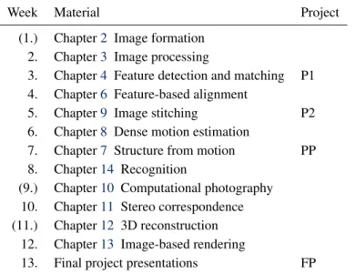
Since that time, a similar syllabus and project-oriented course structure has been used to teach general computer vision courses both at the University of Washington and at Stanford. (The latter was a course I co-taught with David Fleet in 2003.) Similar curricula have been adopted at a number of other universities and also incorporated into more specialized courses on computational photography. (For ideas on how to use this book in your own course, please see Table1.1in Section1.4.)
This book also reflects my 20 years’ experience doing computer vision research in corpo-rate research labs, mostly at Digital Equipment Corporation’s Cambridge Research Lab and at Microsoft Research. In pursuing my work, I have mostly focused on problems and solu-tion techniques (algorithms) that have practical real-world applicasolu-tions and that work well in practice. Thus, this book has more emphasis on basic techniques that work under real-world conditions and less on more esoteric mathematics that has intrinsic elegance but less practical applicability.
technical details are too complex to cover in the book itself.
In teaching our courses, we have found it useful for the students to attempt a number of small implementation projects, which often build on one another, in order to get them used to working with real-world images and the challenges that these present. The students are then asked to choose an individual topic for each of their small-group, final projects. (Sometimes these projects even turn into conference papers!) The exercises at the end of each chapter contain numerous suggestions for smaller mid-term projects, as well as more open-ended problems whose solutions are still active research topics. Wherever possible, I encourage students to try their algorithms on their own personal photographs, since this better motivates them, often leads to creative variants on the problems, and better acquaints them with the variety and complexity of real-world imagery.
In formulating and solving computer vision problems, I have often found it useful to draw inspiration from three high-level approaches:
• Scientific: build detailed models of the image formation process and develop mathe-matical techniques to invert these in order to recover the quantities of interest (where necessary, making simplifying assumption to make the mathematics more tractable).
• Statistical:use probabilistic models to quantify the prior likelihood of your unknowns and the noisy measurement processes that produce the input images, then infer the best possible estimates of your desired quantities and analyze their resulting uncertainties. The inference algorithms used are often closely related to the optimization techniques used to invert the (scientific) image formation processes.
• Engineering: develop techniques that are simple to describe and implement but that are also known to work well in practice. Test these techniques to understand their limitation and failure modes, as well as their expected computational costs (run-time performance).
These three approaches build on each other and are used throughout the book.
My personal research and development philosophy (and hence the exercises in the book) have a strong emphasis ontestingalgorithms. It’s too easy in computer vision to develop an algorithm that does somethingplausibleon a few images rather than somethingcorrect. The best way to validate your algorithms is to use a three-part strategy.
Preface ix
In order to help students in this process, this books comes with a large amount of supple-mentary material, which can be found on the book’s Web sitehttp://szeliski.org/Book. This material, which is described in AppendixC, includes:
• pointers to commonly used data sets for the problems, which can be found on the Web
• pointers to software libraries, which can help students get started with basic tasks such as reading/writing images or creating and manipulating images
• slide sets corresponding to the material covered in this book
• a BibTeX bibliography of the papers cited in this book.
The latter two resources may be of more interest to instructors and researchers publishing new papers in this field, but they will probably come in handy even with regular students. Some of the software libraries contain implementations of a wide variety of computer vision algorithms, which can enable you to tackle more ambitious projects (with your instructor’s consent).
Acknowledgements
I would like to gratefully acknowledge all of the people whose passion for research and inquiry as well as encouragement have helped me write this book.
Steve Zucker at McGill University first introduced me to computer vision, taught all of his students to question and debate research results and techniques, and encouraged me to pursue a graduate career in this area.
Takeo Kanade and Geoff Hinton, my Ph. D. thesis advisors at Carnegie Mellon University, taught me the fundamentals of good research, writing, and presentation. They fired up my interest in visual processing, 3D modeling, and statistical methods, while Larry Matthies introduced me to Kalman filtering and stereo matching.
Demetri Terzopoulos was my mentor at my first industrial research job and taught me the ropes of successful publishing. Yvan Leclerc and Pascal Fua, colleagues from my brief in-terlude at SRI International, gave me new perspectives on alternative approaches to computer vision.
At Microsoft Research, I’ve had the outstanding fortune to work with some of the world’s best researchers in computer vision and computer graphics, including Michael Cohen, Hugues Hoppe, Stephen Gortler, Steve Shafer, Matthew Turk, Harry Shum, Anandan, Phil Torr, An-tonio Criminisi, Georg Petschnigg, Kentaro Toyama, Ramin Zabih, Shai Avidan, Sing Bing Kang, Matt Uyttendaele, Patrice Simard, Larry Zitnick, Richard Hartley, Simon Winder, Drew Steedly, Chris Pal, Nebojsa Jojic, Patrick Baudisch, Dani Lischinski, Matthew Brown, Simon Baker, Michael Goesele, Eric Stollnitz, David Nist´er, Blaise Aguera y Arcas, Sudipta Sinha, Johannes Kopf, Neel Joshi, and Krishnan Ramnath. I was also lucky to have as in-terns such great students as Polina Golland, Simon Baker, Mei Han, Arno Sch¨odl, Ron Dror, Ashley Eden, Jinxiang Chai, Rahul Swaminathan, Yanghai Tsin, Sam Hasinoff, Anat Levin, Matthew Brown, Eric Bennett, Vaibhav Vaish, Jan-Michael Frahm, James Diebel, Ce Liu, Josef Sivic, Grant Schindler, Colin Zheng, Neel Joshi, Sudipta Sinha, Zeev Farbman, Rahul Garg, Tim Cho, Yekeun Jeong, Richard Roberts, Varsha Hedau, and Dilip Krishnan.
While working at Microsoft, I’ve also had the opportunity to collaborate with wonderful colleagues at the University of Washington, where I hold an Affiliate Professor appointment. I’m indebted to Tony DeRose and David Salesin, who first encouraged me to get involved with the research going on at UW, my long-time collaborators Brian Curless, Steve Seitz, Maneesh Agrawala, Sameer Agarwal, and Yasu Furukawa, as well as the students I have had the privilege to supervise and interact with, including Fr´ederic Pighin, Yung-Yu Chuang, Doug Zongker, Colin Zheng, Aseem Agarwala, Dan Goldman, Noah Snavely, Rahul Garg, and Ryan Kaminsky. As I mentioned at the beginning of this preface, this book owes its inception to the vision course that Steve Seitz invited me to co-teach, as well as to Steve’s encouragement, course notes, and editorial input.
Preface xi
tracking down references and finding related work.
If you have any suggestions for improving the book, please send me an e-mail, as I would like to keep the book as accurate, informative, and timely as possible.
Lastly, this book would not have been possible or worthwhile without the incredible sup-port and encouragement of my family. I dedicate this book to my parents, Zdzisław and Jadwiga, whose love, generosity, and accomplishments have always inspired me; to my sis-ter Basia for her lifelong friendship; and especially to Lyn, Anne, and Stephen, whose daily encouragement in all matters (including this book project) makes it all worthwhile.
Contents
Preface vii
Contents xiii
1 Introduction 1
1.1 What is computer vision? . . . 3
1.2 A brief history. . . 10
1.3 Book overview . . . 19
1.4 Sample syllabus . . . 26
1.5 A note on notation . . . 27
1.6 Additional reading . . . 28
2 Image formation 29 2.1 Geometric primitives and transformations . . . 31
2.1.1 Geometric primitives . . . 32
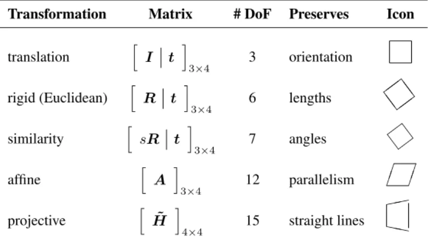
2.1.2 2D transformations . . . 35
2.1.3 3D transformations . . . 39
2.1.4 3D rotations. . . 41
2.1.5 3D to 2D projections . . . 46
2.1.6 Lens distortions. . . 58
2.2 Photometric image formation . . . 60
2.2.1 Lighting. . . 60
2.2.2 Reflectance and shading . . . 62
2.2.3 Optics. . . 68
2.3 The digital camera . . . 73
2.3.1 Sampling and aliasing . . . 77
2.3.2 Color . . . 80
2.4 Additional reading . . . 93
2.5 Exercises . . . 93
3 Image processing 99 3.1 Point operators . . . 101
3.1.1 Pixel transforms . . . 103
3.1.2 Color transforms . . . 104
3.1.3 Compositing and matting. . . 105
3.1.4 Histogram equalization. . . 107
3.1.5 Application: Tonal adjustment . . . 111
3.2 Linear filtering . . . 111
3.2.1 Separable filtering . . . 115
3.2.2 Examples of linear filtering. . . 117
3.2.3 Band-pass and steerable filters . . . 118
3.3 More neighborhood operators. . . 122
3.3.1 Non-linear filtering . . . 122
3.3.2 Morphology . . . 127
3.3.3 Distance transforms . . . 129
3.3.4 Connected components. . . 131
3.4 Fourier transforms . . . 132
3.4.1 Fourier transform pairs . . . 136
3.4.2 Two-dimensional Fourier transforms. . . 140
3.4.3 Wiener filtering . . . 140
3.4.4 Application: Sharpening, blur, and noise removal . . . 144
3.5 Pyramids and wavelets . . . 144
3.5.1 Interpolation . . . 145
3.5.2 Decimation . . . 148
3.5.3 Multi-resolution representations . . . 150
3.5.4 Wavelets . . . 154
3.5.5 Application: Image blending . . . 160
3.6 Geometric transformations . . . 162
3.6.1 Parametric transformations . . . 163
3.6.2 Mesh-based warping . . . 170
3.6.3 Application: Feature-based morphing . . . 173
3.7 Global optimization . . . 174
3.7.1 Regularization . . . 174
3.7.2 Markov random fields . . . 180
Contents xv
3.8 Additional reading . . . 192
3.9 Exercises . . . 194
4 Feature detection and matching 205 4.1 Points and patches. . . 207
4.1.1 Feature detectors . . . 209
4.1.2 Feature descriptors . . . 222
4.1.3 Feature matching . . . 225
4.1.4 Feature tracking . . . 235
4.1.5 Application: Performance-driven animation . . . 237
4.2 Edges . . . 238
4.2.1 Edge detection . . . 238
4.2.2 Edge linking . . . 244
4.2.3 Application: Edge editing and enhancement . . . 249
4.3 Lines . . . 250
4.3.1 Successive approximation . . . 250
4.3.2 Hough transforms. . . 251
4.3.3 Vanishing points . . . 254
4.3.4 Application: Rectangle detection. . . 257
4.4 Additional reading . . . 257
4.5 Exercises . . . 259
5 Segmentation 267 5.1 Active contours . . . 270
5.1.1 Snakes . . . 270
5.1.2 Dynamic snakes and CONDENSATION. . . 276
5.1.3 Scissors . . . 280
5.1.4 Level Sets. . . 281
5.1.5 Application: Contour tracking and rotoscoping . . . 282
5.2 Split and merge . . . 284
5.2.1 Watershed. . . 284
5.2.2 Region splitting (divisive clustering) . . . 286
5.2.3 Region merging (agglomerative clustering) . . . 286
5.2.4 Graph-based segmentation . . . 286
5.2.5 Probabilistic aggregation . . . 288
5.3 Mean shift and mode finding . . . 289
5.3.1 K-means and mixtures of Gaussians . . . 289
5.4 Normalized cuts . . . 296
5.5 Graph cuts and energy-based methods . . . 300
5.5.1 Application: Medical image segmentation . . . 304
5.6 Additional reading . . . 305
5.7 Exercises . . . 306
6 Feature-based alignment 309 6.1 2D and 3D feature-based alignment . . . 311
6.1.1 2D alignment using least squares. . . 312
6.1.2 Application: Panography . . . 314
6.1.3 Iterative algorithms . . . 315
6.1.4 Robust least squares and RANSAC . . . 318
6.1.5 3D alignment . . . 320
6.2 Pose estimation . . . 321
6.2.1 Linear algorithms. . . 322
6.2.2 Iterative algorithms . . . 324
6.2.3 Application: Augmented reality . . . 326
6.3 Geometric intrinsic calibration . . . 327
6.3.1 Calibration patterns. . . 327
6.3.2 Vanishing points . . . 329
6.3.3 Application: Single view metrology . . . 331
6.3.4 Rotational motion . . . 332
6.3.5 Radial distortion . . . 334
6.4 Additional reading . . . 335
6.5 Exercises . . . 336
7 Structure from motion 343 7.1 Triangulation . . . 345
7.2 Two-frame structure from motion. . . 347
7.2.1 Projective (uncalibrated) reconstruction . . . 353
7.2.2 Self-calibration . . . 355
7.2.3 Application: View morphing . . . 357
7.3 Factorization . . . 357
7.3.1 Perspective and projective factorization . . . 360
7.3.2 Application: Sparse 3D model extraction . . . 362
7.4 Bundle adjustment . . . 363
7.4.1 Exploiting sparsity . . . 364
Contents xvii
7.4.3 Uncertainty and ambiguities . . . 370
7.4.4 Application: Reconstruction from Internet photos . . . 371
7.5 Constrained structure and motion. . . 374
7.5.1 Line-based techniques . . . 374
7.5.2 Plane-based techniques. . . 376
7.6 Additional reading . . . 377
7.7 Exercises . . . 377
8 Dense motion estimation 381 8.1 Translational alignment . . . 384
8.1.1 Hierarchical motion estimation. . . 387
8.1.2 Fourier-based alignment . . . 388
8.1.3 Incremental refinement . . . 392
8.2 Parametric motion. . . 398
8.2.1 Application: Video stabilization . . . 401
8.2.2 Learned motion models. . . 403
8.3 Spline-based motion . . . 404
8.3.1 Application: Medical image registration . . . 408
8.4 Optical flow . . . 409
8.4.1 Multi-frame motion estimation. . . 413
8.4.2 Application: Video denoising . . . 414
8.4.3 Application: De-interlacing . . . 415
8.5 Layered motion . . . 415
8.5.1 Application: Frame interpolation. . . 418
8.5.2 Transparent layers and reflections . . . 419
8.6 Additional reading . . . 421
8.7 Exercises . . . 422
9 Image stitching 427 9.1 Motion models . . . 430
9.1.1 Planar perspective motion . . . 431
9.1.2 Application: Whiteboard and document scanning . . . 432
9.1.3 Rotational panoramas. . . 433
9.1.4 Gap closing . . . 435
9.1.5 Application: Video summarization and compression . . . 436
9.1.6 Cylindrical and spherical coordinates . . . 438
9.2 Global alignment . . . 441
9.2.2 Parallax removal . . . 445
9.2.3 Recognizing panoramas . . . 446
9.2.4 Direct vs. feature-based alignment . . . 450
9.3 Compositing. . . 450
9.3.1 Choosing a compositing surface . . . 451
9.3.2 Pixel selection and weighting (de-ghosting) . . . 453
9.3.3 Application: Photomontage . . . 459
9.3.4 Blending . . . 459
9.4 Additional reading . . . 462
9.5 Exercises . . . 463
10 Computational photography 467 10.1 Photometric calibration . . . 470
10.1.1 Radiometric response function . . . 470
10.1.2 Noise level estimation . . . 473
10.1.3 Vignetting. . . 474
10.1.4 Optical blur (spatial response) estimation . . . 476
10.2 High dynamic range imaging . . . 479
10.2.1 Tone mapping. . . 487
10.2.2 Application: Flash photography . . . 494
10.3 Super-resolution and blur removal . . . 497
10.3.1 Color image demosaicing . . . 502
10.3.2 Application: Colorization . . . 504
10.4 Image matting and compositing. . . 505
10.4.1 Blue screen matting. . . 507
10.4.2 Natural image matting . . . 509
10.4.3 Optimization-based matting . . . 513
10.4.4 Smoke, shadow, and flash matting . . . 516
10.4.5 Video matting. . . 518
10.5 Texture analysis and synthesis . . . 518
10.5.1 Application: Hole filling and inpainting . . . 521
10.5.2 Application: Non-photorealistic rendering . . . 522
10.6 Additional reading . . . 524
10.7 Exercises . . . 526
11 Stereo correspondence 533 11.1 Epipolar geometry . . . 537
Contents xix
11.1.2 Plane sweep. . . 540
11.2 Sparse correspondence . . . 543
11.2.1 3D curves and profiles . . . 543
11.3 Dense correspondence . . . 545
11.3.1 Similarity measures. . . 546
11.4 Local methods. . . 548
11.4.1 Sub-pixel estimation and uncertainty. . . 550
11.4.2 Application: Stereo-based head tracking . . . 551
11.5 Global optimization . . . 552
11.5.1 Dynamic programming. . . 554
11.5.2 Segmentation-based techniques . . . 556
11.5.3 Application: Z-keying and background replacement. . . 558
11.6 Multi-view stereo . . . 558
11.6.1 Volumetric and 3D surface reconstruction . . . 562
11.6.2 Shape from silhouettes . . . 567
11.7 Additional reading . . . 570
11.8 Exercises . . . 571
12 3D reconstruction 577 12.1 Shape from X . . . 580
12.1.1 Shape from shading and photometric stereo . . . 580
12.1.2 Shape from texture . . . 583
12.1.3 Shape from focus . . . 584
12.2 Active rangefinding . . . 585
12.2.1 Range data merging . . . 588
12.2.2 Application: Digital heritage . . . 590
12.3 Surface representations . . . 591
12.3.1 Surface interpolation . . . 592
12.3.2 Surface simplification . . . 594
12.3.3 Geometry images . . . 594
12.4 Point-based representations . . . 595
12.5 Volumetric representations . . . 596
12.5.1 Implicit surfaces and level sets . . . 596
12.6 Model-based reconstruction. . . 598
12.6.1 Architecture. . . 598
12.6.2 Heads and faces. . . 601
12.6.3 Application: Facial animation . . . 603
12.7 Recovering texture maps and albedos . . . 610
12.7.1 Estimating BRDFs . . . 612
12.7.2 Application: 3D photography . . . 613
12.8 Additional reading . . . 614
12.9 Exercises . . . 616
13 Image-based rendering 619 13.1 View interpolation. . . 621
13.1.1 View-dependent texture maps . . . 623
13.1.2 Application: Photo Tourism . . . 624
13.2 Layered depth images . . . 626
13.2.1 Impostors, sprites, and layers. . . 626
13.3 Light fields and Lumigraphs . . . 628
13.3.1 Unstructured Lumigraph . . . 632
13.3.2 Surface light fields . . . 632
13.3.3 Application: Concentric mosaics . . . 634
13.4 Environment mattes . . . 634
13.4.1 Higher-dimensional light fields. . . 636
13.4.2 The modeling to rendering continuum . . . 637
13.5 Video-based rendering . . . 638
13.5.1 Video-based animation . . . 639
13.5.2 Video textures . . . 640
13.5.3 Application: Animating pictures . . . 643
13.5.4 3D Video . . . 643
13.5.5 Application: Video-based walkthroughs . . . 645
13.6 Additional reading . . . 648
13.7 Exercises . . . 650
14 Recognition 655 14.1 Object detection . . . 658
14.1.1 Face detection . . . 658
14.1.2 Pedestrian detection . . . 666
14.2 Face recognition. . . 668
14.2.1 Eigenfaces . . . 671
14.2.2 Active appearance and 3D shape models. . . 679
14.2.3 Application: Personal photo collections . . . 684
14.3 Instance recognition. . . 685
Contents xxi
14.3.2 Large databases. . . 687
14.3.3 Application: Location recognition . . . 693
14.4 Category recognition . . . 696
14.4.1 Bag of words . . . 697
14.4.2 Part-based models . . . 701
14.4.3 Recognition with segmentation. . . 704
14.4.4 Application: Intelligent photo editing . . . 709
14.5 Context and scene understanding . . . 712
14.5.1 Learning and large image collections . . . 714
14.5.2 Application: Image search . . . 717
14.6 Recognition databases and test sets . . . 718
14.7 Additional reading . . . 722
14.8 Exercises . . . 725
15 Conclusion 731 A Linear algebra and numerical techniques 735 A.1 Matrix decompositions . . . 736
A.1.1 Singular value decomposition . . . 736
A.1.2 Eigenvalue decomposition . . . 737
A.1.3 QR factorization . . . 740
A.1.4 Cholesky factorization . . . 741
A.2 Linear least squares . . . 742
A.2.1 Total least squares . . . 744
A.3 Non-linear least squares. . . 746
A.4 Direct sparse matrix techniques. . . 747
A.4.1 Variable reordering . . . 748
A.5 Iterative techniques . . . 748
A.5.1 Conjugate gradient . . . 749
A.5.2 Preconditioning. . . 751
A.5.3 Multigrid . . . 753
B Bayesian modeling and inference 755 B.1 Estimation theory . . . 757
B.1.1 Likelihood for multivariate Gaussian noise . . . 757
B.2 Maximum likelihood estimation and least squares . . . 759
B.3 Robust statistics . . . 760
B.4 Prior models and Bayesian inference . . . 762
B.5.1 Gradient descent and simulated annealing . . . 765 B.5.2 Dynamic programming. . . 766 B.5.3 Belief propagation . . . 768 B.5.4 Graph cuts . . . 770 B.5.5 Linear programming . . . 773 B.6 Uncertainty estimation (error analysis) . . . 775
C Supplementary material 777
C.1 Data sets. . . 778 C.2 Software . . . 780 C.3 Slides and lectures . . . 789 C.4 Bibliography . . . 790
References 791
Chapter 1
Introduction
1.1 What is computer vision? . . . 3 1.2 A brief history. . . 10 1.3 Book overview . . . 19 1.4 Sample syllabus . . . 26 1.5 A note on notation . . . 27 1.6 Additional reading . . . 28
(a) (b)
(c) (d)
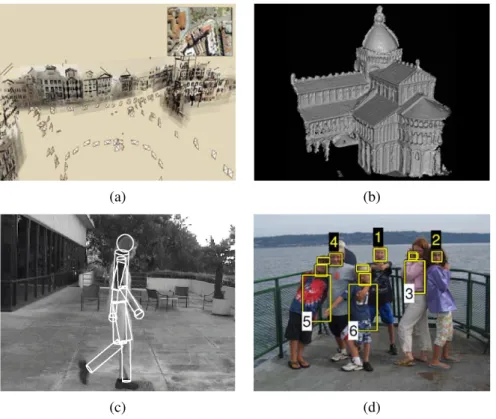
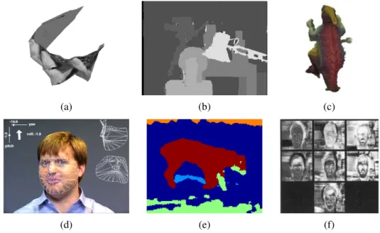
Figure 1.2 Some examples of computer vision algorithms and applications. (a)Structure from motionalgorithms can reconstruct a sparse 3D point model of a large complex scene from hundreds of partially overlapping photographs (Snavely, Seitz, and Szeliski 2006) c 2006 ACM. (b)Stereo matchingalgorithms can build a detailed 3D model of a building fac¸ade from hundreds of differently exposed photographs taken from the Internet (Goesele, Snavely, Curlesset al.2007) c2007 IEEE. (c)Person trackingalgorithms can track a person walking in front of a cluttered background (Sidenbladh, Black, and Fleet 2000) c2000 Springer. (d)
1.1 What is computer vision? 3
1.1 What is computer vision?
As humans, we perceive the three-dimensional structure of the world around us with apparent ease. Think of how vivid the three-dimensional percept is when you look at a vase of flowers sitting on the table next to you. You can tell the shape and translucency of each petal through the subtle patterns of light and shading that play across its surface and effortlessly segment each flower from the background of the scene (Figure1.1). Looking at a framed group por-trait, you can easily count (and name) all of the people in the picture and even guess at their emotions from their facial appearance. Perceptual psychologists have spent decades trying to understand how the visual system works and, even though they can devise optical illusions1 to tease apart some of its principles (Figure1.3), a complete solution to this puzzle remains elusive (Marr 1982;Palmer 1999;Livingstone 2008).
Researchers in computer vision have been developing, in parallel, mathematical tech-niques for recovering the three-dimensional shape and appearance of objects in imagery. We now have reliable techniques for accurately computing a partial 3D model of an environment from thousands of partially overlapping photographs (Figure 1.2a). Given a large enough set of views of a particular object or fac¸ade, we can create accurate dense 3D surface mod-els using stereo matching (Figure1.2b). We can track a person moving against a complex background (Figure1.2c). We can even, with moderate success, attempt to find and name all of the people in a photograph using a combination of face, clothing, and hair detection and recognition (Figure1.2d). However, despite all of these advances, the dream of having a computer interpret an image at the same level as a two-year old (for example, counting all of the animals in a picture) remains elusive. Why is vision so difficult? In part, it is because vision is aninverse problem, in which we seek to recover some unknowns given insufficient information to fully specify the solution. We must therefore resort to physics-based and prob-abilisticmodelsto disambiguate between potential solutions. However, modeling the visual world in all of its rich complexity is far more difficult than, say, modeling the vocal tract that produces spoken sounds.
Theforwardmodels that we use in computer vision are usually developed in physics (ra-diometry, optics, and sensor design) and in computer graphics. Both of these fields model how objects move and animate, how light reflects off their surfaces, is scattered by the at-mosphere, refracted through camera lenses (or human eyes), and finally projected onto a flat (or curved) image plane. While computer graphics are not yet perfect (no fully computer-animated movie with human characters has yet succeeded at crossing theuncanny valley2
that separates real humans from android robots and computer-animated humans), in limited
1http://www.michaelbach.de/ot/sze muelue
(a) (b)
X X X X X X X O X O X O X X
X X X X X X X X O X X X O X
X X X X X X X O X X O X X O
X X X X X X X X X O X O O X
X X X X X X X O X X O X X X
X X X X X X X X O X X X O X
X X X X X X X O X X O X X O
X X X X X X X X O X X X O X
X X X X X X X X X X O O X X
X X X X X X X X O X X X O X
(c) (d)
1.1 What is computer vision? 5
domains, such as rendering a still scene composed of everyday objects or animating extinct creatures such as dinosaurs, the illusion of realityisperfect.
In computer vision, we are trying to do the inverse, i.e., to describe the world that we see in one or more images and to reconstruct its properties, such as shape, illumination, and color distributions. It is amazing that humans and animals do this so effortlessly, while computer vision algorithms are so error prone. People who have not worked in the field often under-estimate the difficulty of the problem. (Colleagues at work often ask me for software to find and name all the people in photos, so they can get on with the more “interesting” work.) This misperception that vision should be easy dates back to the early days of artificial intelligence (see Section1.2), when it was initially believed that thecognitive(logic proving and plan-ning) parts of intelligence were intrinsically more difficult than theperceptualcomponents (Boden 2006).
The good news is that computer visionisbeing used today in a wide variety of real-world applications, which include:
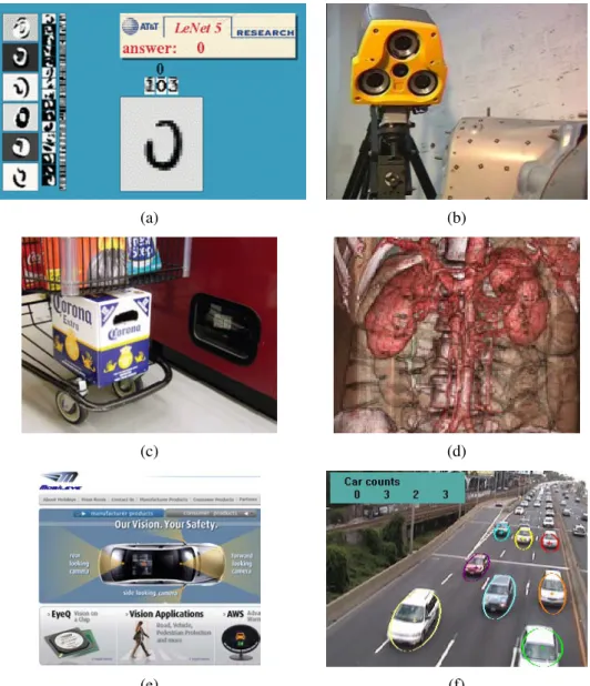
• Optical character recognition (OCR): reading handwritten postal codes on letters (Figure1.4a) and automatic number plate recognition (ANPR);
• Machine inspection: rapid parts inspection for quality assurance using stereo vision with specialized illumination to measure tolerances on aircraft wings or auto body parts (Figure1.4b) or looking for defects in steel castings using X-ray vision;
• Retail:object recognition for automated checkout lanes (Figure1.4c);
• 3D model building (photogrammetry): fully automated construction of 3D models from aerial photographs used in systems such as Bing Maps;
• Medical imaging:registering pre-operative and intra-operative imagery (Figure1.4d) or performing long-term studies of people’s brain morphology as they age;
• Automotive safety: detecting unexpected obstacles such as pedestrians on the street, under conditions where active vision techniques such as radar or lidar do not work well (Figure1.4e; see alsoMiller, Campbell, Huttenlocheret al.(2008);Montemerlo, Becker, Bhatet al.(2008);Urmson, Anhalt, Bagnellet al.(2008) for examples of fully automated driving);
(a) (b)
(c) (d)
(e) (f)
1.1 What is computer vision? 7
• Motion capture (mocap): using retro-reflective markers viewed from multiple cam-eras or other vision-based techniques to capture actors for computer animation;
• Surveillance: monitoring for intruders, analyzing highway traffic (Figure1.4f), and monitoring pools for drowning victims;
• Fingerprint recognition and biometrics: for automatic access authentication as well as forensic applications.
David Lowe’s Web site of industrial vision applications (http://www.cs.ubc.ca/spider/lowe/ vision.html) lists many other interesting industrial applications of computer vision. While the above applications are all extremely important, they mostly pertain to fairly specialized kinds of imagery and narrow domains.
In this book, we focus more on broaderconsumer-levelapplications, such as fun things you can do with your own personal photographs and video. These include:
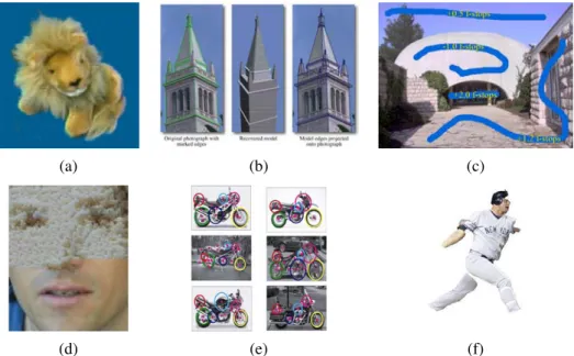
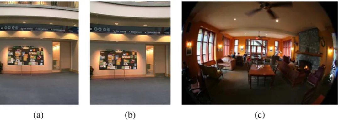
• Stitching:turning overlapping photos into a single seamlessly stitched panorama (Fig-ure1.5a), as described in Chapter9;
• Exposure bracketing: merging multiple exposures taken under challenging lighting conditions (strong sunlight and shadows) into a single perfectly exposed image (Fig-ure1.5b), as described in Section10.2;
• Morphing: turning a picture of one of your friends into another, using a seamless
morphtransition (Figure1.5c);
• 3D modeling: converting one or more snapshots into a 3D model of the object or person you are photographing (Figure1.5d), as described in Section12.6
• Video match move and stabilization: inserting 2D pictures or 3D models into your videos by automatically tracking nearby reference points (see Section7.4.2)3or using motion estimates to remove shake from your videos (see Section8.2.1);
• Photo-based walkthroughs:navigating a large collection of photographs, such as the interior of your house, by flying between different photos in 3D (see Sections13.1.2 and13.5.5)
• Face detection:for improved camera focusing as well as more relevant image search-ing (see Section14.1.1);
(a)
(b)
(c)
(d)
Figure 1.5 Some consumer applications of computer vision: (a) image stitching: merging different views (Szeliski and Shum 1997) c1997 ACM; (b) exposure bracketing: merging different exposures; (c) morphing: blending between two photographs (Gomes, Darsa, Costa
1.1 What is computer vision? 9
The great thing about these applications is that they are already familiar to most students; they are, at least, technologies that students can immediately appreciate and use with their own personal media. Since computer vision is a challenging topic, given the wide range of mathematics being covered4 and the intrinsically difficult nature of the problems being solved, having fun and relevant problems to work on can be highly motivating and inspiring.
The other major reason why this book has a strong focus on applications is that they can be used toformulateandconstrainthe potentially open-ended problems endemic in vision. For example, if someone comes to me and asks for a good edge detector, my first question is usually to askwhy? What kind of problem are they trying to solve and why do they believe that edge detection is an important component? If they are trying to locate faces, I usually point out that most successful face detectors use a combination of skin color detection (Exer-cise2.8) and simple blob features Section14.1.1; they do not rely on edge detection. If they are trying to match door and window edges in a building for the purpose of 3D reconstruction, I tell them that edges are a fine idea but it is better to tune the edge detector for long edges (see Sections3.2.3and4.2) and link them together into straight lines with common vanishing points before matching (see Section4.3).
Thus, it is better to think back from the problem at hand to suitable techniques, rather than to grab the first technique that you may have heard of. This kind of working back from problems to solutions is typical of anengineeringapproach to the study of vision and reflects my own background in the field. First, I come up with a detailed problem definition and decide on the constraints and specifications for the problem. Then, I try to find out which techniques are known to work, implement a few of these, evaluate their performance, and finally make a selection. In order for this process to work, it is important to have realistictest data, both synthetic, which can be used to verify correctness and analyze noise sensitivity, and real-world data typical of the way the system will finally be used.
However, this book is not just an engineering text (a source of recipes). It also takes a scientificapproach to basic vision problems. Here, I try to come up with the best possible models of the physics of the system at hand: how the scene is created, how light interacts with the scene and atmospheric effects, and how the sensors work, including sources of noise and uncertainty. The task is then to try to invert the acquisition process to come up with the best possible description of the scene.
The book often uses astatisticalapproach to formulating and solving computer vision problems. Where appropriate, probability distributions are used to model the scene and the noisy image acquisition process. The association of prior distributions with unknowns is often
3For a fun student project on this topic, see the “PhotoBook” project athttp://www.cc.gatech.edu/dvfx/videos/
dvfx2005.html.
calledBayesian modeling(AppendixB). It is possible to associate a risk or loss function with mis-estimating the answer (SectionB.2) and to set up your inference algorithm to minimize the expected risk. (Consider a robot trying to estimate the distance to an obstacle: it is usually safer to underestimate than to overestimate.) With statistical techniques, it often helps to gather lots of training data from which to learn probabilistic models. Finally, statistical approaches enable you to use proven inference techniques to estimate the best answer (or distribution of answers) and to quantify the uncertainty in the resulting estimates.
Because so much of computer vision involves the solution of inverse problems or the esti-mation of unknown quantities, my book also has a heavy emphasis onalgorithms, especially those that are known to work well in practice. For many vision problems, it is all too easy to come up with a mathematical description of the problem that either does not match realistic real-world conditions or does not lend itself to the stable estimation of the unknowns. What we need are algorithms that are bothrobustto noise and deviation from our models and rea-sonablyefficientin terms of run-time resources and space. In this book, I go into these issues in detail, using Bayesian techniques, where applicable, to ensure robustness, and efficient search, minimization, and linear system solving algorithms to ensure efficiency. Most of the algorithms described in this book are at a high level, being mostly a list of steps that have to be filled in by students or by reading more detailed descriptions elsewhere. In fact, many of the algorithms are sketched out in the exercises.
Now that I’ve described the goals of this book and the frameworks that I use, I devote the rest of this chapter to two additional topics. Section1.2is a brief synopsis of the history of computer vision. It can easily be skipped by those who want to get to “the meat” of the new material in this book and do not care as much about who invented what when.
The second is an overview of the book’s contents, Section1.3, which is useful reading for everyone who intends to make a study of this topic (or to jump in partway, since it describes chapter inter-dependencies). This outline is also useful for instructors looking to structure one or more courses around this topic, as it provides sample curricula based on the book’s contents.
1.2 A brief history
1.2 A brief history 11
Digital im
age
processing
Blocks world, line
labeling Generalized cylinders 197 Generalized cylinders Pictorial structures Stereo correspondence Intrinsic im ages Optical flow Structure from m o tion 70 Im age pyram ids Scale-space processing Shape from shading,
texture, and focus
Physically-based m
odeling 1980 Regularization Markov Random Fields Kalm an f ilters 3D
range data processing Projective invariants
Factorization 1 Factorization Physics-based vision Graph cuts Particle f iltering Ener gy-based segm entation Face recognition and detection 1990 Face recognition and detection Subspace m ethods Im age-based m odeling and rendering T exture synthesis and inpainting Com putational photography 2000
Feature-based recognition MRF inference
algorithm
s
Category recognition
Learning
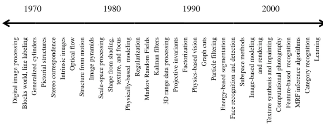
Figure 1.6 A rough timeline of some of the most active topics of research in computer vision.
1970s. When computer vision first started out in the early 1970s, it was viewed as the visual perception component of an ambitious agenda to mimic human intelligence and to endow robots with intelligent behavior. At the time, it was believed by some of the early pioneers of artificial intelligence and robotics (at places such as MIT, Stanford, and CMU) that solving the “visual input” problem would be an easy step along the path to solving more difficult problems such as higher-level reasoning and planning. According to one well-known story, in 1966, Marvin Minsky at MIT asked his undergraduate student Gerald Jay Sussman to “spend the summer linking a camera to a computer and getting the computer to describe what it saw” (Boden 2006, p. 781).5 We now know that the problem is slightly more difficult than that.6
What distinguished computer vision from the already existing field of digital image pro-cessing (Rosenfeld and Pfaltz 1966; Rosenfeld and Kak 1976) was a desire to recover the three-dimensional structure of the world from images and to use this as a stepping stone to-wards full scene understanding. Winston(1975) andHanson and Riseman(1978) provide two nice collections of classic papers from this early period.
Early attempts at scene understanding involved extracting edges and then inferring the 3D structure of an object or a “blocks world” from the topological structure of the 2D lines (Roberts 1965). Severalline labelingalgorithms (Figure1.7a) were developed at that time (Huffman 1971;Clowes 1971;Waltz 1975;Rosenfeld, Hummel, and Zucker 1976;Kanade 1980). Nalwa(1993) gives a nice review of this area. The topic of edge detection was also
5Boden(2006) cites (Crevier 1993) as the original source. The actual Vision Memo was authored by Seymour Papert (1966) and involved a whole cohort of students.
6 To see how far robotic vision has come in the last four decades, have a look at the towel-folding robot at
(a) (b) (c)
(d) (e) (f)
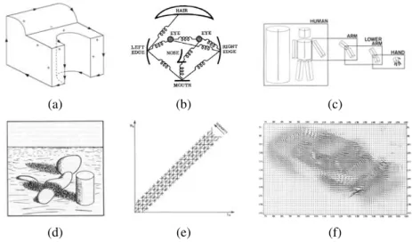
Figure 1.7 Some early (1970s) examples of computer vision algorithms: (a) line label-ing (Nalwa 1993) c1993 Addison-Wesley, (b) pictorial structures (Fischler and Elschlager 1973) c1973 IEEE, (c) articulated body model (Marr 1982) c1982 David Marr, (d) intrin-sic images (Barrow and Tenenbaum 1981) c1973 IEEE, (e) stereo correspondence (Marr 1982) c1982 David Marr, (f) optical flow (Nagel and Enkelmann 1986) c1986 IEEE.
an active area of research; a nice survey of contemporaneous work can be found in (Davis 1975).
Three-dimensional modeling of non-polyhedral objects was also being studied ( Baum-gart 1974;Baker 1977). One popular approach used generalized cylinders, i.e., solids of revolution and swept closed curves (Agin and Binford 1976;Nevatia and Binford 1977), of-ten arranged into parts relationships7(Hinton 1977;Marr 1982) (Figure1.7c). Fischler and Elschlager(1973) called suchelasticarrangements of partspictorial structures(Figure1.7b). This is currently one of the favored approaches being used in object recognition (see Sec-tion14.4andFelzenszwalb and Huttenlocher 2005).
A qualitative approach to understanding intensities and shading variations and explaining them by the effects of image formation phenomena, such as surface orientation and shadows, was championed byBarrow and Tenenbaum(1981) in their paper onintrinsic images (Fig-ure1.7d), along with the related21/2-D sketchideas ofMarr(1982). This approach is again
seeing a bit of a revival in the work ofTappen, Freeman, and Adelson(2005).
More quantitative approaches to computer vision were also developed at the time, in-cluding the first of many feature-based stereo correspondence algorithms (Figure1.7e) (Dev
1.2 A brief history 13
1974;Marr and Poggio 1976;Moravec 1977;Marr and Poggio 1979;Mayhew and Frisby 1981;Baker 1982;Barnard and Fischler 1982;Ohta and Kanade 1985;Grimson 1985; Pol-lard, Mayhew, and Frisby 1985;Prazdny 1985) and intensity-based optical flow algorithms (Figure1.7f) (Horn and Schunck 1981;Huang 1981;Lucas and Kanade 1981;Nagel 1986). The early work in simultaneously recovering 3D structure and camera motion (see Chapter7) also began around this time (Ullman 1979;Longuet-Higgins 1981).
A lot of the philosophy of how vision was believed to work at the time is summarized in David Marr’s (1982) book.8 In particular, Marr introduced his notion of the three levels of description of a (visual) information processing system. These three levels, very loosely paraphrased according to my own interpretation, are:
• Computational theory: What is the goal of the computation (task) and what are the constraints that are known or can be brought to bear on the problem?
• Representations and algorithms: How are the input, output, and intermediate infor-mation represented and which algorithms are used to calculate the desired result?
• Hardware implementation:How are the representations and algorithms mapped onto actual hardware, e.g., a biological vision system or a specialized piece of silicon? Con-versely, how can hardware constraints be used to guide the choice of representation and algorithm? With the increasing use of graphics chips (GPUs) and many-core ar-chitectures for computer vision (see SectionC.2), this question is again becoming quite relevant.
As I mentioned earlier in this introduction, it is my conviction that a careful analysis of the problem specification and known constraints from image formation and priors (the scientific and statistical approaches) must be married with efficient and robust algorithms (the engineer-ing approach) to design successful vision algorithms. Thus, it seems that Marr’s philosophy is as good a guide to framing and solving problems in our field today as it was 25 years ago.
1980s. In the 1980s, a lot of attention was focused on more sophisticated mathematical techniques for performing quantitative image and scene analysis.
Image pyramids (see Section3.5) started being widely used to perform tasks such as im-age blending (Figure1.8a) and coarse-to-fine correspondence search (Rosenfeld 1980;Burt and Adelson 1983a,b;Rosenfeld 1984;Quam 1984;Anandan 1989). Continuous versions of pyramids using the concept ofscale-spaceprocessing were also developed (Witkin 1983; Witkin, Terzopoulos, and Kass 1986;Lindeberg 1990). In the late 1980s, wavelets (see Sec-tion 3.5.4) started displacing or augmenting regular image pyramids in some applications
(a) (b) (c)
(d) (e) (f)
Figure 1.8 Examples of computer vision algorithms from the 1980s: (a) pyramid blending (Burt and Adelson 1983b) c1983 ACM, (b) shape from shading (Freeman and Adelson 1991) c 1991 IEEE, (c) edge detection (Freeman and Adelson 1991) c1991 IEEE, (d) physically based models (Terzopoulos and Witkin 1988) c1988 IEEE, (e) regularization-based surface reconstruction (Terzopoulos 1988) c 1988 IEEE, (f) range data acquisition and merging (Banno, Masuda, Oishiet al.2008) c2008 Springer.
(Adelson, Simoncelli, and Hingorani 1987;Mallat 1989;Simoncelli and Adelson 1990a,b; Simoncelli, Freeman, Adelsonet al.1992).
The use of stereo as a quantitative shape cue was extended by a wide variety of shape-from-Xtechniques, including shape from shading (Figure1.8b) (see Section12.1.1andHorn 1975;Pentland 1984;Blake, Zimmerman, and Knowles 1985;Horn and Brooks 1986,1989), photometric stereo (see Section12.1.1andWoodham 1981), shape from texture (see Sec-tion12.1.2andWitkin 1981;Pentland 1984;Malik and Rosenholtz 1997), and shape from focus (see Section12.1.3andNayar, Watanabe, and Noguchi 1995).Horn(1986) has a nice discussion of most of these techniques.
Research into better edge and contour detection (Figure1.8c) (see Section4.2) was also active during this period (Canny 1986; Nalwa and Binford 1986), including the introduc-tion of dynamically evolving contour trackers (Secintroduc-tion5.1.1) such assnakes(Kass, Witkin, and Terzopoulos 1988), as well as three-dimensionalphysically based models(Figure1.8d) (Terzopoulos, Witkin, and Kass 1987;Kass, Witkin, and Terzopoulos 1988;Terzopoulos and Fleischer 1988;Terzopoulos, Witkin, and Kass 1988).
al-1.2 A brief history 15
gorithms could be unified, or at least described, using the same mathematical framework if they were posed as variational optimization problems (see Section3.7) and made more ro-bust (well-posed) using regularization (Figure1.8e) (see Section3.7.1andTerzopoulos 1983; Poggio, Torre, and Koch 1985;Terzopoulos 1986b;Blake and Zisserman 1987;Bertero, Pog-gio, and Torre 1988;Terzopoulos 1988). Around the same time,Geman and Geman(1984) pointed out that such problems could equally well be formulated using discreteMarkov Ran-dom Field(MRF) models (see Section3.7.2), which enabled the use of better (global) search and optimization algorithms, such as simulated annealing.
Online variants of MRF algorithms that modeled and updated uncertainties using the Kalman filter were introduced a little later (Dickmanns and Graefe 1988;Matthies, Kanade, and Szeliski 1989; Szeliski 1989). Attempts were also made to map both regularized and MRF algorithms onto parallel hardware (Poggio and Koch 1985; Poggio, Little, Gamble
et al.1988; Fischler, Firschein, Barnardet al.1989). The book byFischler and Firschein (1987) contains a nice collection of articles focusing on all of these topics (stereo, flow, regularization, MRFs, and even higher-level vision).
Three-dimensional range data processing (acquisition, merging, modeling, and recogni-tion; see Figure1.8f) continued being actively explored during this decade (Agin and Binford 1976;Besl and Jain 1985;Faugeras and Hebert 1987;Curless and Levoy 1996). The compi-lation byKanade(1987) contains a lot of the interesting papers in this area.
1990s. While a lot of the previously mentioned topics continued to be explored, a few of them became significantly more active.
A burst of activity in using projective invariants for recognition (Mundy and Zisserman 1992) evolved into a concerted effort to solve the structure from motion problem (see Chap-ter7). A lot of the initial activity was directed atprojective reconstructions, which did not require knowledge of camera calibration (Faugeras 1992;Hartley, Gupta, and Chang 1992; Hartley 1994a;Faugeras and Luong 2001;Hartley and Zisserman 2004). Simultaneously, fac-torizationtechniques (Section7.3) were developed to solve efficiently problems for which or-thographic camera approximations were applicable (Figure1.9a) (Tomasi and Kanade 1992; Poelman and Kanade 1997;Anandan and Irani 2002) and then later extended to the perspec-tive case (Christy and Horaud 1996;Triggs 1996). Eventually, the field started using full global optimization (see Section7.4andTaylor, Kriegman, and Anandan 1991;Szeliski and Kang 1994;Azarbayejani and Pentland 1995), which was later recognized as being the same as thebundle adjustmenttechniques traditionally used in photogrammetry (Triggs, McLauch-lan, Hartleyet al.1999). Fully automated (sparse) 3D modeling systems were built using such techniques (Beardsley, Torr, and Zisserman 1996;Schaffalitzky and Zisserman 2002;Brown and Lowe 2003;Snavely, Seitz, and Szeliski 2006).
(a) (b) (c)
(d) (e) (f)
Figure 1.9 Examples of computer vision algorithms from the 1990s: (a) factorization-based structure from motion (Tomasi and Kanade 1992) c1992 Springer, (b) dense stereo match-ing (Boykov, Veksler, and Zabih 2001), (c) multi-view reconstruction (Seitz and Dyer 1999)
c
1999 Springer, (d) face tracking (Matthews, Xiao, and Baker 2007), (e) image segmenta-tion (Belongie, Fowlkes, Chunget al.2002) c2002 Springer, (f) face recognition (Turk and Pentland 1991a).
with accurate physical models of radiance transport and color image formation created its own subfield known asphysics-based vision. A good survey of the field can be found in the three-volume collection on this topic (Wolff, Shafer, and Healey 1992a;Healey and Shafer 1992; Shafer, Healey, and Wolff 1992).
1.2 A brief history 17
Multi-view stereo algorithms (Figure1.9c) that produce complete 3D surfaces (see Sec-tion11.6) were also an active topic of research (Seitz and Dyer 1999;Kutulakos and Seitz 2000) that continues to be active today (Seitz, Curless, Diebelet al.2006). Techniques for producing 3D volumetric descriptions from binary silhouettes (see Section11.6.2) continued to be developed (Potmesil 1987;Srivasan, Liang, and Hackwood 1990;Szeliski 1993; Lau-rentini 1994), along with techniques based on tracking and reconstructing smooth occluding contours (see Section11.2.1andCipolla and Blake 1992;Vaillant and Faugeras 1992;Zheng 1994;Boyer and Berger 1997;Szeliski and Weiss 1998;Cipolla and Giblin 2000).
Tracking algorithms also improved a lot, including contour tracking usingactive contours
(see Section5.1), such assnakes(Kass, Witkin, and Terzopoulos 1988),particle filters(Blake and Isard 1998), andlevel sets(Malladi, Sethian, and Vemuri 1995), as well as intensity-based (direct) techniques (Lucas and Kanade 1981;Shi and Tomasi 1994;Rehg and Kanade 1994), often applied to tracking faces (Figure1.9d) (Lanitis, Taylor, and Cootes 1997;Matthews and Baker 2004;Matthews, Xiao, and Baker 2007) and whole bodies (Sidenbladh, Black, and Fleet 2000;Hilton, Fua, and Ronfard 2006;Moeslund, Hilton, and Kr¨uger 2006).
Image segmentation (see Chapter 5) (Figure1.9e), a topic which has been active since the earliest days of computer vision (Brice and Fennema 1970;Horowitz and Pavlidis 1976; Riseman and Arbib 1977;Rosenfeld and Davis 1979;Haralick and Shapiro 1985;Pavlidis and Liow 1990), was also an active topic of research, producing techniques based on min-imum energy (Mumford and Shah 1989) and minimum description length (Leclerc 1989),
normalized cuts(Shi and Malik 2000), andmean shift(Comaniciu and Meer 2002).
Statistical learning techniques started appearing, first in the application of principal com-ponenteigenfaceanalysis to face recognition (Figure1.9f) (see Section14.2.1andTurk and Pentland 1991a) and linear dynamical systems for curve tracking (see Section5.1.1andBlake and Isard 1998).
(a) (b) (c)
(d) (e) (f)
Figure 1.10 Recent examples of computer vision algorithms: (a) image-based rendering (Gortler, Grzeszczuk, Szeliskiet al.1996), (b) image-based modeling (Debevec, Taylor, and Malik 1996) c1996 ACM, (c) interactive tone mapping (Lischinski, Farbman, Uyttendaele
et al.2006a) (d) texture synthesis (Efros and Freeman 2001), (e) feature-based recognition (Fergus, Perona, and Zisserman 2007), (f) region-based recognition (Mori, Ren, Efroset al.
2004) c2004 IEEE.
2000s. This past decade has continued to see a deepening interplay between the vision and graphics fields. In particular, many of the topics introduced under the rubric of image-based rendering, such as image stitching (see Chapter 9), light-field capture and rendering (see Section13.3), andhigh dynamic range(HDR) image capture through exposure bracketing (Figure1.5b) (see Section10.2andMann and Picard 1995;Debevec and Malik 1997), were re-christened ascomputational photography(see Chapter10) to acknowledge the increased use of such techniques in everyday digital photography. For example, the rapid adoption of exposure bracketing to create high dynamic range images necessitated the development of
1.3 Book overview 19
Dontcheva, Agrawalaet al.2004).
Texture synthesis (Figure1.10d) (see Section10.5), quilting (Efros and Leung 1999;Efros and Freeman 2001; Kwatra, Sch¨odl, Essa et al. 2003) and inpainting (Bertalmio, Sapiro, Caselleset al.2000;Bertalmio, Vese, Sapiroet al.2003;Criminisi, P´erez, and Toyama 2004) are additional topics that can be classified as computational photography techniques, since they re-combine input image samples to produce new photographs.
A second notable trend during this past decade has been the emergence of feature-based techniques (combined with learning) for object recognition (see Section 14.3 andPonce, Hebert, Schmidet al.2006). Some of the notable papers in this area include theconstellation modelof Fergus, Perona, and Zisserman(2007) (Figure1.10e) and thepictorial structures
of Felzenszwalb and Huttenlocher (2005). Feature-based techniques also dominate other recognition tasks, such as scene recognition (Zhang, Marszalek, Lazebniket al.2007) and panorama and location recognition (Brown and Lowe 2007;Schindler, Brown, and Szeliski 2007). And whileinterest point (patch-based) features tend to dominate current research, some groups are pursuing recognition based on contours (Belongie, Malik, and Puzicha 2002) and region segmentation (Figure1.10f) (Mori, Ren, Efroset al.2004).
Another significant trend from this past decade has been the development of more efficient algorithms for complex global optimization problems (see Sections3.7andB.5andSzeliski, Zabih, Scharsteinet al.2008;Blake, Kohli, and Rother 2010). While this trend began with work on graph cuts (Boykov, Veksler, and Zabih 2001;Kohli and Torr 2007), a lot of progress has also been made in message passing algorithms, such asloopy belief propagation(LBP) (Yedidia, Freeman, and Weiss 2001;Kumar and Torr 2006).
The final trend, which now dominates a lot of the visual recognition research in our com-munity, is the application of sophisticated machine learning techniques to computer vision problems (see Section14.5.1andFreeman, Perona, and Sch¨olkopf 2008). This trend coin-cides with the increased availability of immense quantities of partially labelled data on the Internet, which makes it more feasible to learn object categories without the use of careful human supervision.
1.3 Book overview
Images (2D) Geometry (3D) shape + Photometry appearance vision
graphics image processing
2.1 Geometric
image formation
2.2 Photometric
image formation
2.3 Sampling
and aliasing
3 Image
processing
4 Feature
detection
6 Feature-based
alignment
7 Structure
from motion
8 Motion
estimation
10 Computational
photography
11 Stereo
correspondence
12 3D shape
recovery
12 Texture
recovery
13 Image-based
rendering
14 Recognition
5 Segmentation
9Stitching
1.3 Book overview 21
Figure 1.11shows a rough layout of the contents of this book. Since computer vision involves going from images to a structural description of the scene (and computer graphics the converse), I have positioned the chapters horizontally in terms of which major component they address, in addition to vertically according to their dependence.
Going from left to right, we see the major column headings as Images (which are 2D in nature), Geometry (which encompasses 3D descriptions), and Photometry (which encom-passes object appearance). (An alternative labeling for these latter two could also beshape
andappearance—see, e.g., Chapter 13andKang, Szeliski, and Anandan (2000).) Going from top to bottom, we see increasing levels of modeling and abstraction, as well as tech-niques that build on previously developed algorithms. Of course, this taxonomy should be taken with a large grain of salt, as the processing and dependencies in this diagram are not strictly sequential and subtle additional dependencies and relationships also exist (e.g., some recognition techniques make use of 3D information). The placement of topics along the hor-izontal axis should also be taken lightly, as most vision algorithms involve mapping between at least two different representations.9
Interspersed throughout the book are sampleapplications, which relate the algorithms and mathematical material being presented in various chapters to useful, real-world applica-tions. Many of these applications are also presented in the exercises sections, so that students can write their own.
At the end of each section, I provide a set ofexercisesthat the students can use to imple-ment, test, and refine the algorithms and techniques presented in each section. Some of the exercises are suitable as written homework assignments, others as shorter one-week projects, and still others as open-ended research problems that make for challenging final projects. Motivated students who implement a reasonable subset of these exercises will, by the end of the book, have a computer vision software library that can be used for a variety of interesting tasks and projects.
As a reference book, I try wherever possible to discuss which techniques and algorithms work well in practice, as well as providing up-to-date pointers to the latest research results in the areas that I cover. The exercises can be used to build up your own personal library of self-tested and validated vision algorithms, which is more worthwhile in the long term (assuming you have the time) than simply pulling algorithms out of a library whose performance you do not really understand.
The book begins in Chapter2with a review of the image formation processes that create the images that we see and capture. Understanding this process is fundamental if you want to take a scientific (model-based) approach to computer vision. Students who are eager to just start implementing algorithms (or courses that have limited time) can skip ahead to the
n^
2. Image Formation 3. Image Processing 4. Features
5. Segmentation 6-7. Structure from Motion 8. Motion
9. Stitching 10. Computational Photography 11. Stereo
12. 3D Shape 13. Image-based Rendering 14. Recognition
1.3 Book overview 23
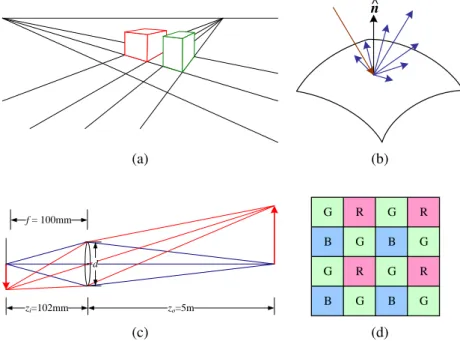
next chapter and dip into this material later. In Chapter2, we break down image formation into three major components. Geometric image formation (Section2.1) deals with points, lines, and planes, and how these are mapped onto images usingprojective geometryand other models (including radial lens distortion). Photometric image formation (Section2.2) covers
radiometry, which describes how light interacts with surfaces in the world, andoptics, which projects light onto the sensor plane. Finally, Section2.3covers how sensors work, including topics such as sampling and aliasing, color sensing, and in-camera compression.
Chapter3covers image processing, which is needed in almost all computer vision appli-cations. This includes topics such as linear and non-linear filtering (Section3.3), the Fourier transform (Section3.4), image pyramids and wavelets (Section3.5), geometric transforma-tions such as image warping (Section3.6), and global optimization techniques such as regu-larizationandMarkov Random Fields(MRFs) (Section3.7). While most of this material is covered in courses and textbooks on image processing, the use of optimization techniques is more typically associated with computer vision (although MRFs are now being widely used in image processing as well). The section on MRFs is also the first introduction to the use of Bayesian inference techniques, which are covered at a more abstract level in AppendixB. Chapter3also presents applications such as seamless image blending and image restoration. In Chapter4, we cover feature detection and matching. A lot of current 3D reconstruction and recognition techniques are built on extracting and matchingfeature points(Section4.1), so this is a fundamental technique required by many subsequent chapters (Chapters6,7,9 and14). We also cover edge and straight line detection in Sections4.2and4.3.
Chapter5covers region segmentation techniques, including active contour detection and tracking (Section 5.1). Segmentation techniques include top-down (split) and bottom-up (merge) techniques, mean shift techniques that find modes of clusters, and various graph-based segmentation approaches. All of these techniques are essential building blocks that are widely used in a variety of applications, including performance-driven animation, interactive image editing, and recognition.
In Chapter6, we cover geometric alignment and camera calibration. We introduce the basic techniques of feature-based alignment in Section6.1and show how this problem can be solved using either linear or non-linear least squares, depending on the motion involved. We also introduce additional concepts, such as uncertainty weighting and robust regression, which are essential to making real-world systems work. Feature-based alignment is then used as a building block for 3D pose estimation (extrinsic calibration) in Section6.2and camera (intrinsic) calibration in Section6.3. Chapter6also describes applications of these techniques to photo alignment for flip-book animations, 3D pose estimation from a hand-held camera, and single-view reconstruction of building models.
fea-tures. This chapter begins with the easier problem of 3D pointtriangulation(Section7.1), which is the 3D reconstruction of points from matched features when the camera positions are known. It then describes two-frame structure from motion (Section7.2), for which al-gebraic techniques exist, as well as robust sampling techniques such as RANSAC that can discount erroneous feature matches. The second half of Chapter7describes techniques for multi-frame structure from motion, including factorization (Section7.3), bundle adjustment (Section7.4), and constrained motion and structure models (Section7.5). It also presents applications in view morphing, sparse 3D model construction, and match move.
In Chapter 8, we go back to a topic that deals directly with image intensities (as op-posed to feature tracks), namely dense intensity-based motion estimation (optical flow). We start with the simplest possible motion models, translational motion (Section8.1), and cover topics such as hierarchical (coarse-to-fine) motion estimation, Fourier-based techniques, and iterative refinement. We then present parametric motion models, which can be used to com-pensate for camera rotation and zooming, as well as affine or planar perspective motion (Sec-tion8.2). This is then generalized to spline-based motion models (Section8.3) and finally to general per-pixel optical flow (Section8.4), including layered and learned motion models (Section8.5). Applications of these techniques include automated morphing, frame interpo-lation (slow motion), and motion-based user interfaces.
Chapter9is devoted toimage stitching, i.e., the construction of large panoramas and com-posites. While stitching is just one example ofcomputation photography(see Chapter10), there is enough depth here to warrant a separate chapter. We start by discussing various pos-sible motion models (Section9.1), including planar motion and pure camera rotation. We then discuss global alignment (Section9.2), which is a special (simplified) case of general bundle adjustment, and then presentpanorama recognition, i.e., techniques for automatically discovering which images actually form overlapping panoramas. Finally, we cover the topics ofimage compositingandblending(Section9.3), which involve both selecting which pixels from which images to use and blending them together so as to disguise exposure differences. Image stitching is a wonderful application that ties together most of the material covered in earlier parts of this book. It also makes for a good mid-term course project that can build on previously developed techniques such as image warping and feature detection and match-ing. Chapter9also presents more specialized variants of stitching such as whiteboard and document scanning, video summarization,panography, full360◦spherical panoramas, and interactive photomontage for blending repeated action shots together.
(Sec-1.3 Book overview 25
tion10.3), and image editing and compositing operations (Section10.4). We also cover the topics of texture analysis, synthesis andinpainting(hole filling) in Section10.5, as well as non-photorealistic rendering (Section10.5.2).
In Chapter11, we turn to the issue of stereo correspondence, which can be thought of as a special case of motion estimation where the camera positions are already known (Sec-tion11.1). This additional knowledge enables stereo algorithms to search over a much smaller space of correspondences and, in many cases, to produce dense depth estimates that can be converted into visible surface models (Section 11.3). We also cover multi-view stereo algorithms that build a true 3D surface representation instead of just a single depth map (Section11.6). Applications of stereo matching include head and gaze tracking, as well as depth-based background replacement (Z-keying).
Chapter12covers additional 3D shape and appearance modeling techniques. These in-clude classicshape-from-Xtechniques such as shape from shading, shape from texture, and shape from focus (Section 12.1), as well as shape from smooth occluding contours (Sec-tion11.2.1) and silhouettes (Section12.5). An alternative to all of thesepassivecomputer vision techniques is to useactive rangefinding(Section12.2), i.e., to project patterned light onto scenes and recover the 3D geometry through triangulation. Processing all of these 3D representations often involves interpolating or simplifying the geometry (Section 12.3), or using alternative representations such as surface point sets (Section12.4).
The collection of techniques for going from one or more images to partial or full 3D models is often calledimage-based modeling or 3D photography. Section 12.6examines three more specialized application areas (architecture, faces, and human bodies), which can usemodel-based reconstructionto fit parameterized models to the sensed data. Section12.7 examines the topic ofappearance modeling, i.e., techniques for estimating the texture maps, albedos, or even sometimes completebi-directional reflectance distribution functions(BRDFs) that describe the appearance of 3D surfaces.
In Chapter 13, we discuss the large number of image-based rendering techniques that have been developed in the last two decades, including simpler techniques such as view in-terpolation (Section13.1), layered depth images (Section13.2), and sprites and layers (Sec-tion 13.2.1), as well as the more general framework of light fields and Lumigraphs (Sec-tion13.3) and higher-order fields such as environment mattes (Section13.4). Applications of these techniques include navigating 3D collections of photographs usingphoto tourismand viewing 3D models asobject movies.