Robust Score Tests With Missing Data in Genomics Studies
Kin Yau Wonga, Donglin Zengb, and D. Y. Linb
aDepartment of Applied Mathematics, The Hong Kong Polytechnic University, Hong Kong;bDepartment of Biostatistics, University of North Carolina, Chapel Hill, NC
ABSTRACT
Analysis of genomic data is often complicated by the presence of missing values, which may arise due to cost or other reasons. The prevailing approach of single imputation is generally invalid if the imputation model is misspecified. In this article, we propose a robust score statistic based on imputed data for testing the association between a phenotype and a genomic variable with (partially) missing values. We fit a semiparametric regression model for the genomic variable against an arbitrary function of the linear predictor in the phenotype model and impute each missing value by its estimated posterior expectation. We show that the score statistic with such imputed values is asymptotically unbiased under general missing-data mechanisms, even when the imputation model is misspecified. We develop a spline-based method to estimate the semiparametric imputation model and derive the asymptotic distribution of the correspond-ing score statistic with a consistent variance estimator uscorrespond-ing sieve approximation theory and empirical process theory. The proposed test is computationally feasible regardless of the number of independent variables in the imputation model. We demonstrate the advantages of the proposed method over existing methods through extensive simulation studies and provide an application to a major cancer genomics study. Supplementary materials for this article are available online.
ARTICLE HISTORY
Received July 2017 Revised May 2018
KEYWORDS
Association tests; Imputation; Integrative analysis; Multiple genomics platforms; Semiparametric models; Sieve estimation
1. Introduction
Recent technological advances have made it possible to measure multiple genomics platforms on the same set of subjects. However, constraints regarding cost and other factors prohibit measurement of all platforms on all study subjects. For example, in The Cancer Genome Atlas (TCGA) (https://cancergenome.nih.gov/), over 10,000 subjects with 33 cancer types were measured on multiple genomics platforms, including somatic mutation, copy number variation, and expressions of microRNA, mRNA, and protein, but for a substantial number of subjects, data on RNA sequencing and protein expressions were not generated. As another example, in the National Heart, Lung, and Blood Institute’s Exome Sequencing Project (https://esp.gs.washington.edu/), only 7000 subjects with specific diseases or conditions were selected for whole-exome sequencing from the tens of thousands of total subjects with genotyping array data (Lin, Zeng, and Tang2013). Finally, in the Trans-Omics for Precision Medicine (TOPMed) program (https://www.nhlbi.nih.gov/research/resources/nhlbi-precision-medicine-initiative/topmed) and the Genome Sequenc-ing Program (GSP;http://gsp-hg.org), whole-genome sequenc-ing data will be available on hundreds of thousands of subjects, but other genomics platforms, such as RNA sequencing, methylation, and metabolites, will be available for only a few thousand subjects through ancillary studies of specific diseases. It is desirable to infer missing data on one genomics platform using available data from other platforms. Indeed, this has become a routine practice with genotype data, where linkage
disequilibrium allows one to impute, with great accuracy, sequencing data from genotyping array data (Li et al. 2010; Auer et al. 2012). A far greater challenge is to infer missing values for a quantitative measurement, such as the expression of RNA or protein, from other quantitative measurements or from SNP genotype data due to the complex and noisy relationships among those variables (Kim, Golub, and Park 2005; Torres-García et al.2009).
Several authors have considered missing data in the context of association testing, which is of primary interest in genomics studies. Specifically, Hu et al. (2015) studied the score test based on imputed genotype data and proposed a variance estima-tor that properly accounts for the differential quality between observed and imputed genotypes. The method requires that the imputation is unbiased and the genotype is independent of the other variables in the phenotype model. Derkach, Lawless, and Sun (2015) and Lawless (2018) proposed to model the variable with missing values under outcome-dependent sampling and studied the score test based on the full likelihood. Derkach, Lawless, and Sun (2015) assumed a nonparametric model for the variable with missing values and restricted covariates to only a few possible values. Lawless (2018) assumed a full paramet-ric missing-data model. All existing methods require unbiased imputation or correct modeling of the variable with missing values. This is difficult to achieve, especially when the number of covariates in the missing-data model is not small.
In this article, we investigate the validity of the score test with imputed data when the missing-data mechanism may depend
on the phenotype and high-dimensional covariates. In particu-lar, we show that a condition weaker than correct specification of the missing-data model is sufficient for the score statistic to be unbiased. Based on this finding, we propose a robust score test which, unlike existing methods, preserves the Type I error under general missing-data mechanisms even when the imputation model is misspecified. The proposed score statistic is based on a semiparametric model for the variable with missing values, where covariates enter the model linearly and also through a one-dimensional nonparametric function. As a result, the test is feasible with a large number of covariates in the missing-data model. The proposed methodology is applicable to all common phenotype models and encompasses continuous, binary, and right-censored phenotypes.
InSection 2, we formulate the problem, investigate the valid-ity of the standard score test under various missing-data mecha-nisms, and develop the robust score test. InSection 3, we report results from simulation studies that compare the proposed and existing methods. We provide an application to a dataset from TCGA in Section 4 and make some concluding remarks in Section 5.
2. Methods
Consider a genomics study that involves phenotypeY, genomic variable of interestS, and vector of covariatesX. For example,Y may represent disease status,Smay represent the RNA expres-sion of a gene, andXmay include genomic variables associated withS, such as the mutation status and copy number of the gene, or nongenomic variables, such as tumor stage, age, and ancestry. Letf(·;βS+γTX,ζ)denote the density function ofY conditional on(S,X), whereβandγare regression parameters, and ζ is a set of nuisance parameters that may be infinite-dimensional; this is referred to as the phenotype model. In particular,ζis the dispersion parameter in the generalized linear model and the baseline hazard function in the proportional hazards model. We allowSto be missing and letRindicate, by values of 1 versus 0, whetherSis observed or not, respectively. LetZ be a set of predictors forS that includesX, as well as variables that are not present in the phenotype model. The extra variables inZ are exogenous variables that affectY indirectly throughSandX, such thatZis independent ofYconditional on Xunderβ =0. The observed data consist of(Yi,SiRi,Ri,Zi)for
i=1,. . .,n.
We are interested in testing the null hypothesisH0 : β =0.
Among the three common tests, namely, the Wald’s test, the likelihood ratio test, and the score test, the first two require fit-ting the model under the alternative hypothesis, which involves estimation of the conditional distribution ofSgivenXin the presence of missing values forS. If the model forSis misspecified (which is inevitable when the dimension of X is moderately high), then the estimators of the nuisance parameters may be inconsistent, such that the resulting tests are invalid. By contrast, the score test only requires fitting the model under the null hypothesis. As a result, the score test requires fewer assumptions on the missing-data model than the other two tests to yield correct Type I error. Therefore, we focus on the score test in the rest of this article.
The score statistic for β at β = 0 takes the form of A(Y,X;ψ)S, whereA(Y,X;ψ)=∂logf(Y;t+γTX,ζ)/∂t|t=0,
andψ = (γ,ζ). Note that E{A(Y,X;ψ0) | X} = 0, where ψ0≡(γ0,ζ0)is the true value ofψ. This formulation includes many common models as special cases. For the linear model, A(Y,X;ψ)= σ−2(Y −γTX), whereσ2is the error variance. For the logistic model,A(Y,X;ψ) = Y −eγTX/(1+eγTX). For the proportional hazards model with right censoring, A(Y,X;ψ) = − (T)eγTX, where Y = (T,), T = min(T,C),=I(T ≤ C),Tis the survival time of interest,C is the censoring time,I(·)is the indicator function, andis the cumulative baseline hazard function.
We consider the score statistic based on the imputedS. We specify an imputation model ofSthat depends onZand a set of parametersξ. LetS(Zi;ξ)be the imputed value ofSi, whereξis
an estimator ofξ. The (normalized) imputation “score” statistic is
Uβimp(ψ,ξ)=n−1/2 n
i=1
A(Yi,Xi;ψ){RiSi+(1−Ri)S(Zi;ξ)},
whereψ ≡ (γ,ζ)is an estimator ofψ underH0. Atβ = 0,
the score statistic based on the full likelihood with a regression model ofSonZtakes the form ofUβimp. However, the proposed
imputation score statistic is more general in thatSneeds not be the posterior mean ofS(given the observed data) evaluated at the maximum likelihood estimator ofξ. Letξ∗ be the limit ofξ. The following proposition provides a general sufficient condition for the unbiasedness of the imputation score statistic underH0.
Proposition 1. Assume that there exists a projection of X, denoted byX, such thatRis independent of(S,Z)conditional on(Y,X)and E(S | γT0X,X) = E{S(Z;ξ∗) | γT0X,X}. Then, E{Uβimp(ψ0,ξ∗)} =0 underβ =0.
The proofs of this proposition and other technical results are provided in Section S.1 of the supplementary materials.
Remark 1. The missing-data mechanism assumed in this proposition may arise from the extreme-tail sampling scheme, where only subjects with extreme values ofY are selected for measurements ofS(Lin, Zeng, and Tang2013). In this case, the inverse probability weighting approach is not feasible because P(R=1|Y)is zero for some subjects, whereas the imputation approach is applicable.
Remark 2. The dependence of R on X may be introduced by design, where the sampling ofSis performed separately at different values ofX. In cancer genomics,Xmay include risk factors such as tumor stage and tumor grade, and subjects with unusually high or unusually low risk may be more likely to be selected for measurements ofS. In addition,Xmay represent categories defined by (possibly continuous) demographic vari-ables such as age. AlthoughX may be high-dimensional and continuous,Xis typically a discrete, low-dimensional projection ofX, such that nonparametric modeling ofSonXis feasible.
given γT0X and X. This condition is trivially satisfied if S is independent ofXand the imputed value has the same mean as S, as assumed by Hu et al. (2015). For the score statistic to be unbiased, we only need the expectation of the true and imputed Svariables conditional onXand a single indexγT0Xto be the same. This is practically achievable via nonparametric model-ing ofSgiven the low-dimensional covariates(γT0X,X), even though the whole set of covariatesXmay be high-dimensional. If the missing-data mechanism does not depend on covariates, then X is absent, such that it is only necessary to correctly model the conditional expectation ofSgiven the single index γT0X.
Proposition 1implies that the imputation score statistic is unbiased underH0 if the conditional expectation of Sgiven
a specific projection of Z (but not necessarily the full set of Z) is correctly specified. To guarantee that this condition holds, we model the relationship between S and (γT0X,X)
nonparametrically whenXis discrete and takes a small number of values. Because the regression model ofSon(γT0X,X)may not be very predictive, we include other components of Z in the imputation model to improve the imputation accuracy. Given the nonparametric function of(γT0X,X), the inclusion of Z will not result in bias of the score statistic even if the imputation model is misspecified. In the sequel, we assume that the missing-data mechanism specified inProposition 1holds and thatXis discrete with possible values(x1,. . .,xL). For each
xl(l = 1,. . .,L), we assume the working model E(S | Z,X =
xl)=gl(γT0X)+ηTlZ, whereglis unspecified, andZis a specific
q-dimensional function ofZthat is (asymptotically) orthogonal to(γT0X,X). Let(gl∗,η∗l) = arg min(gl,ηl)E[R{S−gl(γ
T 0X)−
ηTlZ}2γ0TX,X=xl]almost surely,ξ =(g1,. . .,gL,η1,. . .,ηL),
andξ∗ = (g1∗,. . .,gL∗,η∗1,. . .,η∗L). The following proposition states the unbiasedness of the resulting imputation score statistic.
Proposition 2. IfS(Z;ξ∗)=Ll=1I(X=xl){gl∗(γT0X)+η∗lTZ},
then E{Uβimp(ψ0,ξ∗)} =0.
Proposition 2motivates us to estimateglandηlusing
least-squares regression with the complete observations. We propose to approximategl(l=1,. . .,L) with B-spline functions of order
m(De Boor1978) and replace the true valueγ0by the estimator γ. For simplicity of presentation, we assume the same set of fixed B-spline functions for eachgl, but we allow them to be chosen
adaptively and separately for eachglin practice. LetmandKn
be integers, such thatKn ≥ m ≥ 2, andKndepends on the
sample sizen. For a set of grid pointsτ ≡ (τ0,. . .,τKn−m+1),
such that minXγTX = τ0 < · · · < τKn−m+1 = maxXγ
TX,
letB(·) = (B1(·),. . .,BKn(·))T, whereBk is thekthm-order
B-spline function onτ; the grid points at the two ends have multiplicitym. Forl=1,. . .,L, let
(αl,ηl)=arg min (αl,ηl)
1 2
n
i=1
RiI(Xi=xl)
×
Si−
Kn
k=1
αlkBk(γTXi)−ηTlZi
2
,
whereαl = (αl1,. . .,αlKn)
T. Effectively, we partition the data
intoLstrata, with each stratum corresponding to a value ofxl,
and we perform separate least-squares regression for each stra-tum using subjects with observedS. Letαl =(αl1,. . .,αlKn)
T,
gl =
Kn
k=1αlkBk, andξ =(g1,. . .,gL,η1,. . .,ηL). The robust
imputation score statistic isUβrob(ψ,ξ;γ), where
Uβrob(ψ,ξ;γ)=n−1/2 n
i=1
A(Yi,Xi;ψ) RiSi+(1−Ri)
×
L
l=1
I(Xi=xl){gl(γTXi)+ηTlZi}
,
and the third argument inUβrob(ψ,ξ;γ)corresponds toγin the argument ofgl.
Let β(ψ,ξ;γ) be Uβrob(ψ,ξ;γ) for a single subject, ψ(ψ)[h1] be the derivative of logf(Y;γTX,ζ) along the
pathψ = ψ0 +h1, with h1 being a tangent vector for ψ, βψ(ψ,ξ;γ)[h1] be the derivative of β(ψ,ξ;γ) along the
same path, ψψ(ψ)[h1,h2] be the derivative of ψ(ψ)[h1]
along the path ψ = ψ0 + h2, with h2 being a tangent
vector forψ, and ξ(ξ)[h3]be the derivative ofRLl=1I(X =
xl){S −gl(γT0X)−ηTlZ}2/2 along the path ξ = ξ∗ +h3,
with h3 being a tangent vector for ξ. Let Pn and P denote
the empirical and true probability measures, respectively. We impose the following conditions.
(C1) Forl=1,. . .,L,gl∗andη∗l are unique, andgl∗has bounded fourth derivative.
(C2) The support ofZ is bounded, and γT0Xhas a bounded continuous support. Conditional onZ,Shas finite second moment.
(C3) The number of knots of the B-spline functions is such that Kn6n−1/2→0 andKn7n−1/2→ ∞asn→ ∞.
(C4) Atβ =0,ζ−ζ0 =op(n−1/4)for a suitable norm, and
the estimatorγ satisfies
γ−γ0=Pn ∗γ(ψ0)+op(n−1/2),
where ∗γ is the efficient score function ofγ, such that
P ∗γ(ψ0)=0, andP γ∗(ψ0) ∗γ(ψ0)Tis nonzero and finite.
(C5) The functions 2β(ψ,ξ;γ0), 2ψ(ψ)[h1], βψ(ψ,ξ;γ0)[h1],
and ψψ(ψ)[h1,h2]are Donsker for(ψ,ξ)belonging to
a neighborhood of (ψ0,ξ∗)and (h1,h2)belonging to a
bounded subset of a suitable metric space. In addition, the information operator for the phenotype model P ψψ(ψ0)[·,·]is invertible under the null hypothesisH0.
Remark 4. Conditions (C1) and (C2) pertain to regularity conditions on the variable with missing values and covariates. Forgl∗andη∗l to be unique, we require thatXandγT0Xcannot be expressed as functions of linear terms of Z. In practice, we letZbe a linear combination of the components ofZ not present in X, such that ni=1ZiZTiγ = 0. Condition (C3)
pertains to the rate at which the number of knots of the B-spline functions increases to infinity; particularly, the condition is satisfied withKn =O(n1/13). Conditions (C4) and (C5) are
proportional hazards models. For parametric models and the Cox proportional hazards model, the norm in condition (C4) is the Euclidean norm and the ∞[0,t∗]-norm, respectively, where t∗is the end of the study, and the metric space for(h1,h2)in
condition (C5) is the Euclidean space and the space of functions of bounded variation, respectively.
The asymptotic distribution of the robust imputation score statistic is given in the following theorem.
Theorem 1. Under conditions (C1)–(C5) and β = 0, Uβrob(ψ,ξ;γ)is asymptotically zero-mean normal with variance
V=P[{ β(ψ0,ξ∗;γ0)− ψ(ψ0)[hψ] − ξ(ξ∗)[hξ]
−Iγ(γ0,ξ∗)T ∗γ(ψ0)}2],
wherehψsolvesP βψ(ψ0,ξ∗;γ0)[·] =P ψψ(ψ0)[hψ,·],hξ = (hg,1. . .,hg,L,hη,1,. . .,hη,L), such thathη,l=0and
hg,l(t)=
E{(1−R)I(X=xl)A(Y,X;ψ0)|γT0X=t,X=xl}
E{RI(X=xl)|γT0X=t,X=xl}
forl=1,. . .,L,
Iγ(γ,ξ)= L
l=1
E
I(X=xl)X{Rgl(γTX)hg,l(γTX)
−(1−R)A(Y,X;ψ)gl(γTX)}
,
andf denotes the first derivative off for any functionf.
Remark 5. The second and third terms inV are projections of the score function of (ψ,ξ), and hψ is the least-favorable
direction ofψfor the phenotype model if the imputation model is assumed to be known. The fourth term inVis present because γ, instead of the true value, is used in the imputation model. The estimatorγ affects the imputation both by directly entering the imputation functiongl(γTX)and by involving in the estimation
ofgl.
Motivated byTheorem 1, we propose an empirical variance estimator of the score statistic
V=n−1
n
i=1
{ β,i(ψ,ξ;γ)− ψ,i(ψ)[hψ] − ξ,i(ξ)[hξ]
−Iγ(ψ,ξ)∗γ(ψ)} −M
2
,
where( β,i, ψ,i, ξ,i)is ( β, ψ, ξ)evaluated at the observa-tions of theith subject,Mis the sample mean of the term in the curly brackets inV, and(hψ,hξ,Iγ,∗γ)is the empirical version
of(hψ,hξ,Iγ, ∗γ)evaluated at(ψ,ξ). Specifically,hξis obtained
by performing the usual linear expansion ofξ atξ∗, with the imputation model treated as a linear model with covariates I(X =xl)(B(γTX)T,Z
T
)T. The explicit form ofhξ is given in
the proof of Theorem 2 in Section S.1 of the supplementary materials. We formulate the variance estimator under the linear model, the logistic model, and the Cox proportional hazards model in Section S.2 of the supplementary materials. The result-ing score test statistic isUβrob(ψ,ξ;γ)2/V. The validity of the robust score test is stated below.
Theorem 2. Under conditions (C1)–(C5) andβ =0, the empir-ical variance estimatorV converges almost surely to the true varianceV, and the test statisticUβrob(ψ,ξ;γ)2/Vconverges in distribution to the chi-square distribution with one degree of freedom.
Remark 6. The empirical variance estimator is consistent regardless of the missing-data mechanism and the imputation model. By contrast, the standard model-based variance estima-tor with imputed data is generally biased if the missing-data mechanism depends on the phenotype. The bias of the standard variance estimator under generalized linear models is derived in Section S.3 of the supplementary materials.
When the missing-data mechanism does not depend on the phenotype, the score statistic is unbiased under any imputation schemes; this result follows from the proof ofProposition 1. In this case, the proposed test is not required for bias correction, and one may wonder whether the inclusion of the B-spline terms and the stratification may lead to power loss. The comparison of power between the proposed test and the standard score test under general settings is difficult, because the power generally depends on the missing-data mechanism and high moments of S; the derivation for the power of the proposed test is given in Section S.4 of the supplementary materials. WhenYis normally distributed andSis missing completely at random, the asymp-totic power of the proposed test is higher than or equal to that of the standard score test, because the imputation model with the B-spline terms, stratification, and linear predictors may have a better fit than the model with the linear predictors alone.
3. Simulation Studies
LetX = (X1,X2,X3)T, whereX1,X2, andX3 are independent
standard normal, Bernoulli(0.5), and Binomial(2, 0.25), respec-tively. Let G be a vector of other covariates that are used to predict S. In particular, G = (G1,. . .,G4)T, where Gj (j =
1,. . ., 4) is independent Binomial(2, 0.3). In cancer genomics, X1,X2, andX3may represent (standardized) age, gender, and
tumor stage, respectively, andGmay represent genotypes at four loci. We generated the phenotypeY using the linear predictor r(S,X)=γ0+γTX+βSunder the linear, logistic, and
propor-tional hazards models. For all models, we setγ =(1,−1, 0.5)T. For the linear model, we generatedY∼N{r(S,X), 1}withγ0=
0. For the logistic model, we set logit−1{P(Y = 1 | S,X)} =
r(S,X), whereγ0was chosen such thatP(Y = 1) ≈ 0.15. For
the proportional hazards model, we generatedYwith the hazard functionλ(t | S,X) = 0.5ter(S,X)andγ0 = 0. The censoring variable was generated independently from Unif(0,τ ), where
τ was chosen such that the censoring proportion was about 40%. We considered two models for S: with Model 1, S = X1+X2 +0.3X3 +0.4(G1 −G2 +G3−G4)+N(0, 1); and
with Model 2,S = (X1+X2)+0.1(X1 +X2)2 +0.3I(X3 =
2)+0.4(G1−G2+G3−G4)+N(0, 1).
and a random sample of subjects from the subset were selected for observation ofS; the other subset consisted of all subjects withX2 = 0, and subjects from the subset were selected for
observation ofSbased on the phenotype. For the continuous and survival phenotypes, an equal number of subjects at the two extreme tails of the phenotype distribution were selected. For the binary phenotype, all subjects withY = 1 were selected, and a fraction of subjects withY = 0 were selected to attain the desired missing proportion. The missing proportion was set to be the same between the two subsets of subjects. This setting mimics a study where two datasets with different sam-pling schemes are combined. For Mechanism 3, four strata were defined with X ≡ 3j=0I(X1 > zj/4) denoting the
stratum number, where zα is the α-quantile of the standard
normal distribution. Subjects were selected for observation ofS separately for each stratum using the sampling scheme adopted for the second subset of subjects in Mechanism 2. The missing proportion was set to be the same across strata. This setting was designed to evaluate the sensitivity of the proposed test to misspecification ofX.
We compared the performance of six tests: (1) the standard score test using complete data only; (2) the standard score test with missing values imputed under a linear model ofSonZ≡
(XT,GT)T; (3) Lawless’s (2018) score test based on the same model of S as (2); (4) Hu et al.’s (2015) score test with the imputed data of (2); (5) the proposed score test withZbeing that specified inRemark 4and with stratification variableX=X2for
Mechanisms 1 and 2 orX=I(X1 >0)for Mechanism 3; and
(6) the imputation score test with missing data imputed using a linear model ofSonZ = (XT,X21,X1X2,I(X3 =2),GT)Tand
the empirical variance estimator. We refer to methods (1)–(6) as the complete-case analysis, the simple imputation method, Law-less’ method, Hu’s method, the proposed imputation method, and the full-model imputation method, respectively. The last method is the gold standard but is not practical because it requires correct specification of a complex missing-data model. Derkach, Lawless, and Sun’s (2015) method was not included because it requires the covariates in the imputation model to be discrete and is identical to Lawless’s (2018) method when a linear imputation model is assumed. Note that the missing-data models used by all the methods are correct under Model 1, but only the missing-data model used by the full-model imputation method is correct under Model 2. For the proposed imputation method, we chose the degree and number of knots of the B-spline functions using five-fold cross-validation separately for each stratum. For thelth stratum, the grid pointτk (k =
1,. . .,Kn−m−2) was set to be the empiricalk/(Kn−m+1)
-quantile ofγTXi among subjects withRi = 1 andXi = xl, τ0 =minXi=xlγ
TX
i, andτKn−m−1 =maxXi=xlγ
TX
i. Lawless’
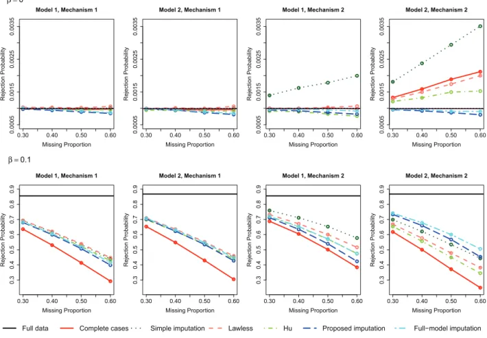
and Hu’s methods are not applicable to the survival phenotype. We considered a sample size of 1500 and missing propor-tions ranging from 30% to 60%. For each setting, we simulated 1,000,000 and 100,000 replicates for β = 0 and β = 0, respectively. The nominal significance level was set to 10−3. We plot the rejection probability against the missing proportion for the two models ofSand the three missing-data mechanisms. For reference, the rejection probability of the score test based on the full data (i.e., no missing values) is also shown. For Mechanisms 1 and 2, the results of the linear model are displayed inFigure 1,
and the results of the logistic and Cox proportional hazards models are displayed in Figures S1–S2 of the supplementary materials. For Mechanism 3, the results are shown in Figures S3–S5 of the supplementary materials.
Under Mechanism 1, all methods have correct Type I error. Under Model 1 and Mechanism 2, the simple imputation method has inflated Type I error because the variance of the score statistic is underestimated. The complete-case analysis is also invalid except for the binary phenotype, but the Type I error inflation is not as severe; the complete-case analysis for the binary phenotype has correct Type I error because of the special structure of the logistic model (Prentice and Pyke 1979). Hu et al.’s (2015) variance estimator requires that both the actual and imputedSvariables are independent ofX, which does not hold under either Model 1 or Model 2. As a result, the variance is overestimated under Mechanism 2, which leads to Type I error deflation. The remaining methods have consistent variance estimators and, therefore, have correct Type I error. Under Model 2 and Mechanism 2, the score statistics of the complete-case analysis and the methods based on a model ofS on linear terms ofXare generally biased, giving rise to Type I error inflation in most cases. Hu’s method exhibits Type I error deflation under the logistic model because the bias of the score statistic is offset by the overestimation of the variance in this specific setting. (Because the absolute bias of the score statistic tends to infinity asn → ∞, Hu’s method would yield Type I error inflation for large enough sample size.) The proposed imputation method is valid even though the imputation model is misspecified because the score statistic is unbiased. The full-model imputation method is also valid because the imputation model is correct. Note that the proposed imputation method and the full-model imputation method exhibit Type I error deflation when the missing proportion is large. This is probably because the two methods involve a relatively large number of parameters, such that the normal approximations to the score statistics are inaccurate when the effective sample size is small.
The power of the complete-case analysis is generally low because it discards useful information. Under Model 1 or Mech-anism 1, all valid methods that use the whole dataset have similar power. Under Model 2 and Mechanism 2, the full-model imputation method is the most powerful among the valid methods because a correct imputation model is assumed. However, this method cannot be used in practice because it requires knowledge of the true relationship betweenSandZ. The proposed imputation method is only slightly less powerful than the full-model imputation method. The bias of the score statistic of the other methods can lead to substantially low power.
Figure 1. Rejection probabilities for the continuous phenotype under the null and alternative hypotheses for Mechanisms 1 and 2.
the proposed test is robust against misspecification ofX, so that strata with too few data points can be collapsed.
4. Real Data Analysis
We analyzed a dataset of patients with serous ovarian cancer from TCGA (The Cancer Genome Atlas Research Network 2011). In the study, most subjects had available genomic data, including data on DNA copy number, somatic mutation, and levels of expression of mRNA measured by microarray plat-forms. Only a subset of subjects had enough tissue sample left for RNA sequencing, which was introduced after the study had begun. Demographic and clinical variables, including age at diagnosis, tumor stage, tumor grade, time to tumor progression, and time to death, were available for most subjects. The median follow-up time was about 2.5 years, and roughly 30% of the patients were lost to follow-up before tumor progression or death. The data are available athttp://gdac.broadinstitute.org/.
We focused on testing the association between mRNA expression, measured by RNA sequencing, and progression-free survival time. We used the fragments per kilobase of transcript per million mapped reads values for the mRNA expression variable. The number of transcripts with RNA sequencing data was about 57,000. We considered a subset of 9068 genes that were mutated in samples from more than five subjects. The number of subjects with available mutation, copy number, and clinical data was 407, approximately 30% of whom did not have RNA sequencing data.
We fit the Cox model for progression-free survival and included age, age squared, tumor stage, tumor grade, the interaction between age and (dichotomized) tumor stage, and the interaction between age and (dichotomized) tumor grade as covariates. Because the missing-data status is significantly associated with tumor stage (with a p-value of 4.83×10⁻⁶) but not with the other covariates, we set the stratification variableX to be (dichotomized) tumor stage. The predictors in the imputation model of the RNA sequencing data included age, age squared, somatic mutation, copy number, and mRNA microarray expression; tumor stage and tumor grade were not included because their inclusion would render the estimation of the imputation model unstable. Microarray mRNA expression and somatic mutation were excluded from the imputation model if they were missing or too sparse. The B-spline functions were selected in the same way as in the simulation studies. For comparison, we performed the standard score test with only the complete cases and with the missing values imputed under a linear model. For further illustration, we performed the proposed test and the standard score test on the dataset with the missing proportion increased to 60%, where the RNA sequencing variables for subjects with intermediate survival or censoring time were treated as missing. The quantile-quantile plots are shown inFigure 2.
Figure 2.Quantile-quantile plots for the RNA-seq analysis of the TCGA ovarian cancer data. The left plot shows the results for the original data, and the right plot shows the results with the missing proportion increased to 60%. Thep-values are truncated at 10−10.
Table 1. Top genes in the RNA-seq analysis of the TCGA ovarian cancer data.
Proposed Complete Simple
Gene method cases imputation Reference
WDR91 1.60E−05 3.20E−04 2.65E−05 N/A
SLC4A8 1.06E−04 7.77E−05 1.08E−05 N/A
SCEL 3.82E−04 8.86E−04 6.29E−03 N/A
DUSP1 6.73E−04 1.26E−03 2.63E−03 Denkert et al. (2002)
VMO1 7.94E−04 9.06E−02 4.24E−03 N/A
PDLIM3 9.25E−04 1.15E−02 3.19E−03 Mougeot et al. (2006)
Bignotti et al. (2007)
PLAUR 9.87E−04 5.38E−03 9.40E−04 Arend et al. (2013)
DCN 9.98E−04 1.67E−02 2.40E−03 Sherman-Baust et al. (2003)
CNTN4 1.22E−03 1.22E−01 1.32E−02 de Cristofaro et al. (2016)
MARK3 1.38E−03 2.53E−03 3.80E−04 N/A
NOTE: The top 10 genes identified by the proposed method are given in the first column, and theirp-values under the proposed method, the complete-case analysis, and the simple imputation method are given in the second to fourth columns. The references for studies that have identified an association between each gene and ovarian cancer, if available, are given in the last column. “N/A” means that no prior studies that identified such an association can be found.
excessive false-positive signals because the standard variance estimates of the score statistic are smaller than the empirical variance. With extra missing data, the inflation of Type I error is more severe for the simple imputation method, whereas the Type I error is preserved by the proposed method.
The top 10 genes identified by the proposed method are presented in Table 1. Several of them have been previously known to be associated with ovarian cancer, with references given inTable 1. Among these genes, the associations between progression-free survival time and the expressions of all genes except SLC4A8 are more significant under the proposed method than under the complete-case analysis. The significance levels for the associations between progression-free survival time and the expressions of WDR91, SCEL, DUSP1, VMO1, PDLIM3, DCN, CNTN4, and MARK3 are lower under the simple impu-tation method than under the proposed method.
5. Discussion
In this article, we propose a robust score test for the association between a phenotype and a genomic variable with partially missing values. The test is based on a semiparametric model for the genomic variable, where the semiparametric component ensures that under the null hypothesis, the score statistic with imputed values is unbiased for general missing-data
mechanisms and arbitrary distributions of the genomic variable. Because each nonparametric function gl in the imputation
model is a one-dimensional function of the covariates, the score test is computationally feasible with a large number of covariates provided thatLis small. In addition to correcting for the bias of the score statistic, the semiparametric component results in a better fit of the imputation model, which leads to power gain even when data are missing completely at random. When the missing-data mechanism depends on the phenotype, the proposed test has correct Type I error, whereas the standard score test is generally invalid. When the missing-data mechanism is independent of the phenotype, both the proposed and standard score tests have correct Type I error, but the proposed test is asymptotically more powerful.
not hold under the alternative hypothesis, making parameter estimation with missing data a much more challenging problem than hypothesis testing. For estimation, single imputation gen-erally yields underestimation of standard errors (Little1992), and a correct specification of the missing-data model is required for valid inference.
Multiple imputation (Rubin1987) is an alternative to single imputation. To perform multiple imputation, the distribution of Sconditional on the observed data, including the phenotype, has to be correctly specified. By contrast, correct specification of the distribution ofSgiven a low-dimensional function of the covariateXis sufficient for the proposed test to be valid. Thus, multiple imputation requires much stronger assumptions than the proposed test. In fact, multiple imputation with the missing values imputed from the (correct) conditional distribution ofS givenXis invalid (Little1992).
Our work can be extended in several directions. First, we have focused on a continuous genomic variable that is either exactly observed or missing. We may allow for a binary or cat-egorical variable by incorporating the proposed semiparamet-ric component into a generalized linear modeling framework. We may also consider genomic variables that are subject to censoring or detection limits, as in the case of metabolomics data (Yu et al. 2014). In this case, the conditional mean of the genomic variable cannot be consistently estimated using simple least-squares estimation, and additional assumptions on the distribution of the genomic variable are necessary.
Second, it would be of interest to perform a joint test for multiple genomic variables, where each variable may have a separate pattern of missing values. This extension can be applied to many existing testing procedures that involve a multivariate score statistic, such as the sequence kernel association test for rare variants (Wu et al.2011), tests for meta-analysis of sequenc-ing data (Tang and Lin 2013), and the joint test for multiple genomic variables (Huang, VanderWeele, and Lin2014). Joint modeling of multiple variables with missing values is more challenging than modeling a single variable with missing value, when the pattern of the missing values for each variable do not overlap. Nevertheless, fitting a separate imputation model for each variable is not preferable, as it results in efficiency loss when the variables are correlated.
Finally, we have assumed that the missing-data mechanism depends only on the phenotype and a set of discrete covariates. The methodology can be extended to allow the missing-data mechanism to depend on continuous covariates by relating the variable with missing values to a nonparametric function of the phenotype and covariates. In addition, we may consider a missing-data mechanism that depends on a different phenotype; this scenario is common in the analysis of secondary pheno-types. In this case, the function through which the covariates affect the alternative phenotype must be estimated, and the vari-able with missing values should be modeled nonparametrically on that function.
Supplementary Materials
The supplementary materials contain proofs of the technical results, explicit forms ofV, derivation for the bias of the standard variance estimator, eval-uation of the power of the imputation score test, and additional simulation results.
Funding
This research was supported by the National Institutes of Health grants R01GM047845, R01HG009974, and P01CA142538.
References
Arend, R. C., Londoño-Joshi, A. I., Straughn, J. M. Jr, and Buchsbaum, D. J. (2013), “The Wnt/β-Catenin Pathway in Ovarian Cancer: A Review,”
Gynecologic Oncology, 131, 772–779. [1784]
Auer, P. L., Johnsen, J. M., Johnson, A. D., Logsdon, B. A., Lange, L. A., Nalls, M. A., Zhang, G., Franceschini, N., Fox, K., Lange, E. M., Nalls, M. A., Zhang, G., Franceschini, N., Fox, K., Lange, E. M., Rich, S. S., O’Donnell, C. J., Jackson, R. D., Wallace, R. B., Chen, Z., Graubert, T. A., Wilson, J. G., Tang, H., Lettre, G., Reiner, A. P., Ganesh, S. K., and Li, Y. (2012), “Imputation of Exome Sequence Variants Into Population-Based Samples and Blood-Cell-Trait-Associated Loci in African Amer-icans: NHLBI GO Exome Sequencing Project,”The American Journal of
Human Genetics, 91, 794–808. [1778]
Bignotti, E., Tassi, R. A., Calza, S., Ravaggi, A., Bandiera, E., Rossi, E., Donzelli, C., Pasinetti, B., Pecorelli, S., and Santin, A. D. (2007), “Gene Expression Profile of Ovarian Serous Papillary Carcinomas: Identifica-tion of Metastasis-Associated Genes,”American Journal of Obstetrics &
Gynecology, 196, 245-e1–245.e11. [1784]
De Boor, C. (1978),A Practical Guide to Splines, New York: Springer. [1780] de Cristofaro, T., Di Palma, T., Soriano, A. A., Monticelli, A., Affinito, O., Cocozza, S., and Zannini, M. (2016), “Candidate Genes and Pathways Downstream of PAX8 Involved in Ovarian High-Grade Serous Carci-noma,”Oncotarget, 7, 41929–41947. [1784]
Denkert, C., Schmitt, W. D., Berger, S., Reles, A., Pest, S., Siegert, A., Lichtenegger, W., Dietel, M., and Hauptmann, S. (2002), “Expression of Mitogen-Activated Protein Kinase Phosphatase-1 (MKP-1) in Primary Human Ovarian Carcinoma,”International Journal of Cancer, 102, 507– 513. [1784]
Derkach, A., Lawless, J. F., and Sun, L. (2015), “Score Tests for Association Under Response-Dependent Sampling Designs for Expensive Covari-ates,”Biometrika, 102, 988–994. [1778,1782]
Hu, Y. J., Li, Y., Auer, P. L., and Lin, D. Y. (2015), “Integrative Analysis of Sequencing and Array Genotype Data for Discovering Disease Asso-ciations With Rare Mutations,”Proceedings of the National Academy of Sciences, 112, 1019–1024. [1778,1780,1782]
Huang, Y. T., VanderWeele, T. J., and Lin, X. (2014), “Joint Analysis of SNP and Gene Expression Data in Genetic Association Studies of Complex Diseases,”The Annals of Applied Statistics, 8, 352–376. [1785]
Kim, H., Golub, G. H., and Park, H. (2005), “Missing Value Estimation for DNA Microarray Gene Expression Data: Local Least Squares Imputa-tion,”Bioinformatics, 21, 187–198. [1778]
Lawless, J. (2018), “Two-Phase Outcome-Dependent Studies for Failure Times and Testing for Effects of Expensive Covariates,”Lifetime Data Analysis, 24, 28–44. [1778,1782]
Li, Y., Willer, C. J., Ding, J., Scheet, P., and Abecasis, G. R. (2010), “MaCH: Using Sequence and Genotype Data to Estimate Haplotypes and Unob-served Genotypes,”Genetic Epidemiology, 34, 816–834. [1778] Lin, D. Y., Zeng, D., and Tang, Z. Z. (2013), “Quantitative Trait Analysis
in Sequencing Studies Under Trait-Dependent Sampling,”Proceedings of
the National Academy of Sciences, 110, 12247–12252. [1778,1779]
Little, R. J. (1992), “Regression With Missing X’s: A Review,”Journal of the
American Statistical Association, 87, 1227–1237. [1785]
Mougeot, J.-L. C., Bahrani-Mostafavi, Z., Vachris, J. C., McKinney, K. Q., Gurlov, S., Zhang, J., Naumann, R. W., Higgins, R. V., and Hall, J. B. (2006), “Gene Expression Profiling of Ovarian Tissues for Determi-nation of Molecular Pathways Reflective of Tumorigenesis,”Journal of
Molecular Biology, 358, 310–329. [1784]
Prentice, R. L., and Pyke, R. (1979), “Logistic Disease Incidence Models and Case-Control Studies,”Biometrika, 66, 403–411. [1782]
Rubin, D. B. (1987), Multiple Imputation for Nonresponse in Surveys, New York: Wiley. [1785]
of the Extracellular Matrix Through Overexpression of Collagen VI Contributes to Cisplatin Resistance in Ovarian Cancer Cells,”Cancer Cell, 3, 377–386. [1784]
Tang, Z. Z., and Lin, D. Y. (2013), “MASS: Meta-Analysis of Score Statistics for Sequencing Studies,”Bioinformatics, 29, 1803–1805. [1785] The Cancer Genome Atlas Research Network (2011), “Integrated
Genomic Analyses of Ovarian Carcinoma,” Nature, 474, 609–615. [1783]
Torres-García, W., Zhang, W., Runger, G. C., Johnson, R. H., and Meldrum, D. R. (2009), “Integrative Analysis of Transcriptomic and Proteomic
Data of Desulfovibrio Vulgaris: A Non-Linear Model to Predict Abun-dance of Undetected Proteins,”Bioinformatics, 25, 1905–1914. [1778] Wu, M. C., Lee, S., Cai, T., Li, Y., Boehnke, M., and Lin, X. (2011),
“Rare-Variant Association Testing for Sequencing Data With the Sequence Kernel Association Test,”The American Journal of Human Genetics, 89, 82–93. [1785]