Soft-Sphere Continuum Solvation in Electronic-Structure
Calculations
Giuseppe Fisicaro,*
,†Luigi Genovese,
‡Oliviero Andreussi,
¶,§Sagarmoy Mandal,
∥Nisanth N. Nair,
∥Nicola Marzari,
§and Stefan Goedecker
††Department of Physics, University of Basel, Klingelbergstrasse 82, CH-4056 Basel, Switzerland ‡Laboratoire de simulation atomistique (L_Sim), SP2M, INAC, CEA-UJF, F-38054 Grenoble, France
¶Institute of Computational Science, Universitàdella Svizzera Italiana, Via Giuseppe Buffi13, CH-6904 Lugano, Switzerland §Theory and Simulations of Materials (THEOS) and National Centre for Computational Design and Discovery of Novel Materials
(MARVEL), École Polytechnique Fedé rale de Lausanne, Station 12, CH-1015 Lausanne, Switzerland́ ∥Department of Chemistry, Indian Institute of Technology Kanpur, Kanpur 208016, India
*
S Supporting InformationABSTRACT: We present an implicit solvation approach where the interface between the quantum-mechanical solute and the surrounding environment is described by a fully continuous permittivity built up with atomic-centered “soft” spheres. This approach combines many of the advantages of the self-consistent continuum solvation model in handling solutes and surfaces in contact with complex dielectric environments or electrolytes in electronic-structure calcula-tions. In addition it is able to describe accurately both neutral and charged systems. The continuous function, describing the variation of the permittivity, allows to compute analytically the nonelectrostatic contributions to the solvation free energy that are described in terms of the quantum surface. The whole
methodology is computationally stable, provides consistent energies and forces, and keeps the computational efforts and runtimes comparable to those of standard vacuum calculations. The capabilitiy to treat arbitrary molecular or slab-like geometries as well as charged molecules is key to tackle electrolytes within mixed explicit/implicit frameworks. We show that, with given,
fixed atomic radii, two parameters are sufficient to give a mean absolute error of only 1.12 kcal/mol with respect to the experimental aqueous solvation energies for a set of 274 neutral solutes. For charged systems, the same set of parameters provides solvation energies for a set of 60 anions and 52 cations with an error of 2.96 and 2.13 kcal/mol, respectively, improving upon previous literature values. To tackle elements not present in most solvation databases, a new benchmark scheme on wettability and contact angles is proposed for solid−liquid interfaces and applied to the investigation of the stable terminations of a CdS (112̅0) surface in an electrochemical medium.
1. INTRODUCTION
The computational study of matter in various environments is a continuously growingfield in solid-state physics and chemistry. Systems of interest are for instance molecules, clusters, or surfaces in contact with solvents.1 A possibility is to include explicitly in the simulation domain all the atoms and molecules of the solution. Such an explicit treatment is in principle the natural way to account for solvent effects in afirst-principles scheme. However, this approach enormously increases the computational cost and limits at the same time the size of the system contained in the explicit dielectric medium.2 As a consequence, the study of the solute−solvent interactions at length scales larger than molecular sizes, or the generation of long molecular dynamics trajectories, requires big computa-tional efforts.
Numerically expensive investigations in material science such as structure predictions3 or reaction path determinations4 would become very time-consuming if not altogether unaffordable. During an exploration of the potential energy surface, most of the minima would arise from rearrangements of solvent molecule. For an hydrated surface, a lot of time would consequently be spent moving water molecules rather than sampling the solid−water interface that is of interest. The explicit description of water also suffers from some well-known limitations of current state-of-the-art ab initio methods, in particular regarding its structural and dielectric properties.5−8
The alternative is an implicit description of the solvent effects, while still treating the other parts of the system
Received: April 10, 2017
Published: June 19, 2017
pubs.acs.org/JCTC
explicitly on an atomic level. Such an explicit/implicit treatment requires three main ingredients:
• A dielectric cavity represented by a proper functionϵ(r) mimicking the surrounding solvent of a solute as a continuum dielectric;
• A solver for the generalized Poisson equation:9
ϕ πρ
∇·ϵ( )r ∇ ( )r = −4 ( )r (1)
whereϕ(r) is the potential generated by a given charge densityρ(r);
• A model for the nonelectrostatic terms to the total free energy of solvation.
The dielectric function ϵ(r) has to take the value of one where the solute is placed to solve a vacuum-like quantum problem and the bulk dielectric constantϵ0outside.
Several implicit solvation models have been reported in the quantum chemistry literature, starting from the earliest work of Onsager10 to the widespread polarizable continuum model (PCM) developed by Tomasi and co-workers.11−13
In the PCM formulation, the cavity surrounding the solute is described by a sharp and discontinuous dielectric functionϵ(r), and a polarization charge density is exactly localized at the interface between the vacuum and the dielectric. In this way, the dielectric environment is represented by an effective surface polarization charge, reducing the three-dimensional dielectric problem into a two-dimensional one. In its original formulation, this approach suffers from discontinuities in the atomic forces and numerical singularities that are a consequence of sharp cavities. This drawback hindered a PCM extension to ab initio molecular dynamics (MD). Modified versions have been proposed in the literature14,15as well as advanced definitions of the dielectric cavity in terms of an isodensity of the solute charge density.16,17
Another possibility is to represent the interface between the region inside the cavity and the implicit solvent region outside the cavity by a smooth function of the solute electronic density ρ(r).18−20 Nonelectrostatic contributions to the solvation free energy can be expressed as a function of the cavity volume and surface area.19,21,22For a charge-dependent approach ϵ[ρ](r), the functional derivative with respect to ρ(r) of the Hamiltonian delivers new additional terms to the Kohn− Sham (KS) potential, both from the electrostatic energy and the nonelectrostatic contributions.22 These formulations are elegant and easy to be parametrized. The cavity changes self-consistently during the wave function optimization, and forces do not depend explicitly on the shape of the cavity. However, there are a number of drawbacks. The smooth transition between the quantum and continuum regions gives rise to an inherently three-dimensional problem, while the self-consistent nature of the approach requires solving a new problem at each step of electronic optimization; thus the approach is intrinsi-cally computationally more demanding than the rigid 2D alternatives such as PCM. Moreover, accuracy might be affected due to the low number of parameters; neutral and charged molecules cannot be treated simultaneously, as these require different parametrizations,23 which lead to different Hamil-tonians. Furthermore, it is not possible to locally modify cavity sizes looking only to the electronic density.
Greater flexibility can be added to these smooth functional approaches by defining them in terms of afictitious electronic density, which is kept rigid and defined in terms of parametrized functions centered at atomic positions.24
Although this approach may overcome some of the computa-tional limitations of self-consistent alternatives, its original formulation only focused on the electrostatic terms of the solvation free energy.
To make a mixed explicit/implicit treatment attractive to material science, it is necessary to fulfill several requirements:
• Accurate forces and a numerical cost comparable to standard vacuum calculations to make MD or extensive potential energy surface (PES) explorations feasible; • A small number of cavity parameters, in order to easilyfit
a new environment orfind the best solvent conditions in a given range;
• Exact treatment of molecular or slab-like geometries, typical of systems plunged in a solvent;
• Ability to treat neutral and charged molecules simulta-neously, in order to tackle complex interfaces (e.g., a double layer).
The self-consistent continuum solvation (sccs) model developed by Andreussi et al.22goes in this direction, satisfying the first three conditions. In the present work an improved implicit solvation model is proposed. It preserves theflexibility of PCM to locally vary the cavity’s size around each atom as well as the straightforward definition of the nonelectrostatic contributions to the total energy of the charge-dependent solvation models and function of the cavity volume and surface.22 The dielectric cavity is based on analytic smooth spheres centered on each atom, and it is fully continuous from the vacuum-like inner regions to the external bulk solvent. Because of these features, we named our approach the“ soft-sphere” model. The proposed formulation satisfies all the requirements listed above. It gives the same accuracy for the ionic forces as an ordinary vacuum calculation. Compared to the similar approache of Sanchez et al.,24 that is based on functionals of afictitious solute density, our definition of the cavity in terms of atom-centered smooth functions simplifies significantly the calculation of derivatives. In addition, the continuous function, describing the variation of the permittiv-ity, allows us to compute analytically all the nonelectrostatic contributions to the free energy. Once wefix the atomic radii, a given environment can be fitted with two parameters in a straightforward way. Details of the model will be presented in
Section 2.
Our implementation has a small numerical overhead, thanks to an efficient solver for the generalized Poisson equation,9 based on a preconditioned conjugate gradient (PCG) algorithm.
The method has been tested within KS density functional theory (DFT) as implemented in the BigDFT package.25,26 Thanks to the underlining electrostatic solver of this package,27 the solvation problem for slab or isolated systems is solved with the correct boundary conditions. An extensive parametrization study has been carried out both for neutral molecules and ions in water and two nonaqueous solvents. Results are reported in
Section 3.
Our tests suggest that our approach can well handle slab-like boundary conditions. InSection 4we propose a benchmarking database for slab-like geometries that is based on the wetting properties and solvent contact angles of solvated surfaces. Standard protocols parametrize implicit solvation models on a database of experimental free solvation energies for neutral and ionic solutes in several solvents.28However, if applied to solid− liquid interfaces in material science, several issues arise. The Journal of Chemical Theory and Computation
molecules of the standard benchmark sets have a limited representation of some elements of the periodic table. Many of these underrepresented elements, such as transition-metal atoms, play however an important role in many materials science problems. Solar-energy harvesting in dye-sensitized29 and hybrid cells30,31 or electrocatalytic water splitting32,33 are just two simple examples where such materials are extensively exploited.
Finally, as an illustrative application of the approach, we present a test case of relevance in material science, namely the prediction of stable terminations of the CdS (112̅0) surface in an electrochemical medium.
2. SOFT-SPHERE MODEL
The electrostatic solvation energy is defined as the difference between the total energy of a given atomic system in the presence of the dielectric environmentGeland the energy of the same system in vacuumG0:
ΔGel= Gel−G0 (2)
A full comparison with experimental solvation energies needs the inclusion of nonelectrostatic contributions to obtain the total free energy of solvationΔGsol. In this case the main terms
in the solute Hamiltonian, as introduced by PCM,12are
ΔGsol = ΔGel+Gcav+ Grep+Gdis + ΔGtm+ ΔP V
(3)
where ΔGel is the electrostatic contribution, and Gcav is the
cavitation energy, i.e., the energy necessary to build up the solute cavity inside the solvent medium.Grepis a repulsion term
representing the continuum counterpart of the short-range interactions induced by the Pauli exclusion principle, while the dissociation energyGdisreflects van der Waals interactions. The thermal termΔGtmaccounts for the vibrational and rotational
changes and,finally,PΔVincludes volume changes in the solute Hamiltonian.
In the case of a charge density-dependent cavity, it has been shown that the nonelectrostatic termsGcav,Grep, andGdiscan be
expressed as linear functions of the “quantum surface” S and “quantum volume”Vof the dielectric cavity.19,22In particular, Scherlis et al.19 extended the work of Fattebert and Gygi18 including a cavitation term expressed as a product of the experimental surface tension of the solventγand the quantum surfaceSof the solute cavity:
γ =
Gcav S (4)
Both the quantum surface and volume can be expressed in terms of the dielectric function ϵ(r). Neglecting, as in other models, the thermal contributionΔGtmto the total energy and
considering that for simulations at standard pressure the term
PΔVdoes not play any role, the total solvation free energy can be modeled by the following expression:22
α γ β
ΔGsol = ΔGel+( + )S+ V (5)
where α and β are solvent-specific parameters which can be
fitted to experimental data such as solvation energies of neutral molecules and ions. The linear relation between the repulsion energy and the quantum surface follows the idea of traditional PCM approaches, since in PCM modelsGrepis proportional to the solute electronic density lying outside the dielectric cavity34 and this last quantity can be linearly correlated to the cavity surface. The linear model for the nonelectrostatic terms follows the same lines as the solvation models developed by Cramer
and Truhlar,13,35i.e., the SMxfamily, where these contributions are evaluated as a sum over all the atoms, each one proportional to the solvent-accessible surface area, albeit they use more variables. Althougheq 5has been introduced within a charge-dependent model,22 we will use the same expression for the total solvation free energy for the soft-sphere model after a suitable generalization of the quantum surface and volume. These last nonelectrostatic contributions do not change during the wave function optimization as they do not depend anymore on the electronic charge density (now the dielectric cavity is a function of the atomic coordinates). As a consequence, only the electrostatic contribution Gel needs to be computed via an optimization of the electronic wave function at the ab initio level.Appendix A outlines the main equations that have to be implemented in a DFT code for the wave function optimization procedure in the presence of an implicit environment.
The spatially varying dielectric functionϵ[ρ](r) orϵ(r,{Ri}) has to meet several conditions:
• Go monotonically from a value of 1 inside the cavity (mimicking vacuum) to the bulk dielectric constantϵ0;
• Be smooth in the transition region to guarantee a proper discretization on a three-dimensional grid;
• Have as many continuous derivatives as possible to avoid convergence and numerical issues during the iterative wave function optimization loop.
The soft-sphere cavity, which satisfies all these requirements, will be presented in Section 2.1. Definitions of the quantum surface and volume will be given inSection 2.2.
For a dielectric cavity whereϵ(r,{Ri}) is an explicit function of the atomic coordinatesRi, additional contributions arise to the atomic forces with respect to their gas-phase formulation. Formulas for the forces are presented inAppendix A.3. A test for the energy and force accuracy is reported onSection 2.3.
The methodology described in this paper as well as a complementary method based on a charge density-dependent continuum solvation model, developed by Andreussi et al.,22 have been implemented in the BigDFT software package.
2.1. Definition of the Dielectric Cavity. We define the soft-sphere cavity by means of atomic-centered interlocking spheres described by continuous and differentiable hfunctions which smoothly switch from 0 inside the sphere to the value 1 outside. Their product, which is still continuous and diff er-entiable in the whole domain, reproduces the analytic cavity:
∏
ξϵ = ϵ − − +
⎪ ⎪
⎪ ⎪
⎧ ⎨ ⎩
⎫ ⎬ ⎭
h
r R r R
( , { })i ( 1) ({ }; ) 1
i
i 0
(6)
whereϵ0is the dielectric constant of the surrounding medium,
{ξ} is a set of parameters describing the spheres, and∥r−Ri∥
is the distance from the sphere centerRi. The derivative of the dielectric function with respect toRiis
ξ
ξ
∂ϵ
∂ =
ϵ −
−
∂ −
∂ ⎡
⎣
⎢ ⎤
⎦ ⎥
h
h r R
R
r R r R
r R R
( , { }) ( , { }) 1
({ }; )
({ }; )
i i
i i
i i
(7)
for a given functionh. This function can be expressed in terms of the error function:
Δ − = + − −
Δ ⎡
⎣
⎢ ⎛⎝⎜ ⎞⎠⎟⎤ ⎦ ⎥
h r( , ; r R ) 1 r R r
2 1 erf
i i
i i
(8)
Journal of Chemical Theory and Computation
where ri are the sphere radii which depend on the particular atomic species, andΔis a parameter (fixed for all atoms) which controls the transition region (≈ 4Δ wide) where the polarization charge is located. This choice for h guarantees a “soft” dielectric function in eq 6 that is analytic everywhere except at the point r = Ri. With our choice of Δ, the discontinuities in the derivatives are however exponentially small and do not have any negative effect on our calculations. Following the lines of all PCM implementations,11,12,35,36ri
are taken to be equal to the van der Waals radii rivdWof the corresponding elements scaled by a constant multiplying factor
f(i.e.,ri=f rivdW). Finally, the soft-sphere cavity for a system of atoms with coordinates Ri is uniquely defined by the set of parameters {ϵ0, rivdW, Δ, f}. The solvation model needs three additional parametersα,β, andγfor the nonelectrostatic terms to the total solvation energy (eq 5). The parametrization of all parameters will be reported onSection 3.
2.2. Geometrical Contributions. Eq 3 allows us to compute the total free energy of solvation. Thanks toeq 5the integration at DFT level of the nonelectrostatic terms becomes straightforward. The evaluation of the free energy and its functional derivative can be expressed in term of the quantum surface and volume. Introducing the function
θ ϵ = ϵ − ϵ
ϵ −
r r
[ ]( ) ( )
1
0
0 (9)
which takes a value of one inside the dielectric cavity and zero externally. The quantum volumeVof the solute can be defined as
∫
θϵ = ϵ
V[ ] d [ ]( )r r
(10)
The integral has to be evaluated in the whole simulation domain. The associated quantum surfaceScan be defined from the gradient ofθ[ϵ]:21
∫
θ∫
ϵ = |∇ ϵ | =
ϵ − |∇ϵ |
S[ ] dr [ ]( )r 1 r r
1 d ( )
0 (11)
The functional derivatives of the quantum volume and surface with respect to the dielectric function are
δ δ
ϵ
ϵ = −ϵ −
V r
[ ] ( )
1 1
0 (12)
∫
δ δ
δ δ
ϵ
ϵ = ϵ − ′
∂ ϵ ′ ϵ
∂ ϵ ′ |∇ϵ ′ |
= ϵ −
∂ ϵ ∂ ϵ ∂ ∂ ϵ
|∇ϵ | −
∇ ϵ |∇ϵ | ⎛
⎝
⎜⎜ ⎞⎠⎟⎟
S
r r
r r
r r
r r r
r
r r
[ ] ( )
1
1 d
( ) ( )
( ) ( )
1 1
( ) ( ) ( )
( )
( ) ( )
i i
i j i j
0
0 3
2
(13)
where repeated indices are considered as summed.
Thanks to the continuous and differentiable permittivityϵ(r), the functionθ[ϵ](r) as well as the quantum volume and surface can be analytically computed. This holds also for their derivatives ofeqs 11−13.
2.3. Energy and Force Accuracy.Accurate energies and forces are fundamental, especially for MD and structure prediction calculations. Smooth and analytical cavities can guarantee accuracy levels comparable to the ones in vacuum.
Appendix A.3shows the additional terms to the forces for the soft-sphere model. These can be analytically computed (seeeq 48). In addition, it is worth noting that all these analytic
contributions to the forces can be computed once during a wave function optimization.
The extent of the transition region (≈4Δwide) can affect the energy and force accuracy. A largeΔcan lead to a nonphysical superposition of large dielectric cavities, while a small value can require a high-resolution mesh which becomes computationally expensive. As a consequence, a compromise is needed, considering the more mesh points that fall in the transition region, the more accurate is the description of solvent effects over the solute and the polarization charge there located. In the following, we report a test of the energy and force accuracy for a water molecule in implicit water. Details of the model’s parameter setting will be given inSection 3. In the present test we used the parametrization reported in row 3 ofTable 1.
Forces can be tested by means of the test-forces tool of BigDFT, an internal program which compares the variation of the total energyΔEwith the path integral of the forces−Fa·dra. As consequence ofeq 46, their differenceδ=ΔE+∑aFa·dra should be zero. Due to the finite discretization and the numerical integration, such value depends on the three-dimensional spatial grid [hx, hy, hz] of the simulation domain (where the KS problem is solved). It reachesδ∼ 10−6Ha in gas phase for very accurate calculations. Typical values of hi (withi =x,y,z) are in most cases between 0.3 and 0.6 bohr. Present test runs make use of an uniform grid spacing in all three directions, i.e.,hgrid: =hx= hy=hz.Figure 1a shows the accuracyδof the force computation as a function ofΔ. Solid lines represent the value ofδfor a test-forces run of the H2O
molecule in vacuum for a givenhgrid. The accuracy of the forces
is comparable to that of vacuum runs, forΔvalues between 0.2 and 0.8 au; deviations start to take place atΔ= 0.1 au, while smaller values affect the convergence of the generalized Poisson solver due to the increased sharpness of the transition region. In Figure 1b we reported the accuracy of the solvation free energyΔGsol, i.e., eq 5, for the same set of calculations. The
accuracy is defined as the difference between values extracted for a givenhgridand the most accurate grid we tested athgrid=
0.2 au. VaryingΔthe same accuracy is recovered forhgrid≥0.4
au. Ahgrid = 0.4 au guarantees an accuracy of 10−2kcal/mol.
Similar results obtained with other small organic molecules lead to similar conclusions. Performance of the soft-sphere model is discussed inAppendix Bfor the same system.
3. PARAMETRIZATION
The soft-sphere solvation model is defined by the parameter set {ζ} = {ϵ0,rivdW,Δ,f;α,β,γ}, i.e., six parameters plus an atomic radius rivdW for each distinct atomic species of the quantum
system in contact with the implicit solvent. Only thefirst four
Table 1. MAEs in Aqueous Solvation Free Energies (kcal/ mol) for a Set of 274 Neutral Molecules Obtained with the Soft-Sphere Solvation Model
atomic radii
rivdW
cavity multiplying
factorf α
+γ
[dyn/cm] [GPa]β
MAE [kcal/mol]
UFF48 1.12 50.0 −0.35 1.10
UFFa 1.16 11.5 0.00 1.12
UFFa 1.12 50.0 −0.35 1.03
Pauling47 1.36 50.0 −0.35 1.17
Bondi46 1.32 50.0 −0.35 1.06
aThe van der Waals atomic radii from the UFF setup48with Bondi’s
radius46for nitrogen.
Journal of Chemical Theory and Computation
parameters are related to the dielectric cavity and the electrostatic contribution ΔGel. To parametrize the solvation model, we need to map the {ζ} = {ϵ0, rivdW, Δ, f; α, β, γ}
parameter space and minimize the mean absolute error (MAE) over a given collection of experimental free solvation energies. In the following we will report the parametrization for a water environment, both for neutral molecules and ions. In addition, we have parametrized two nonaqueous solvents, namely mesitylene and ethanol. Structures and experimental data have been retrieved from the Minnesota Solvation Database, version 2012.28,37−39 Solutes used as benchmark contain at most the following elements: H, C, N, O, F, Si, P, S, Cl, Br, and I.
Soft norm-conserving pseudopotentials including a nonlinear core correction40,41 along with PBE functional were used to describe the core electrons and exchange−correlation for all
calculations of the present section. The Libxc42 library was exploited for the calculation of the functionals. Solvation free energies were computed via eq 5 using atomic structures optimized both in vacuum and in the presence of the implicit solvent. BigDFT represents the wave function in a wavelet basis set. These basis functions are centered on a Cartesian mesh of resolution [hx,hy,hz].25The generalized Poisson equation, i.e.,
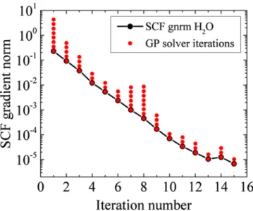
eq 1, has been solved via the recently developed generalized Poisson solver based on interpolating scaling functions.9 Its preconditioner, based on the BigDFT vacuum Poisson solver, allows to solve the electrostatic problem in some 10 iterations with an exact treatment of free, surface, and periodic boundary conditions.27,43A new version of the algorithm which includes a proper use of an input guess is reported in Appendix B. All simulations reported in the present study use an uniform grid of
hx=hy=hz = 0.40 au and free boundary conditions.
3.1. Neutral Molecules. The soft-sphere model has been benchmarked on a collection of 274 aqueous solvation free energies to reproduce a water environment. Atfirst, to speed up the exploration of the parameter space, we trained the model on a representative subset, which consists of 13 molecules spanning the main functional groups of the entire set.44
3.1.1. Cavity Parameters.In order to reduce the size of the
parameter space (in principle a MAE should be extracted for each {ζ } setup), we proceeded fixing the largest possible number of parameters. Since we are benchmarking the model on aqueous solvation free energies, the experimental value at low frequency and ambient conditions ofϵ0= 78.36 has been
used. A critical point in PCM approaches is the choice of shape and size of the cavity, which should reflect the charge distribution of the solute. In the first formulation of this model,45PCM atomic radiiriwere chosen to be proportional to the van der Waals radii.46,47Importing a consistent set of van der Waals radii rivdW which spans the whole periodic table is
more meaningful thanfitting radii for all the elements which would presumably lead to some overfitting. We decided to import rivdW from the unified force field (UFF) parametriza-tion48 for all elements of the periodic table. Hydrogen atoms have been considered explicit in the present work, andΔhas beenfixed to 0.5 au for all atoms, generating a transition region of≈2 au. Different choices of Δwill be also investigated and discussed at the end of the paragraph. Finally, only the multiplying factor f for the atomic radii are left free to vary, reducing the four-parameter problem for the cavity definition to a single-parameter optimization.
Theflexibility to locally change atomic radii has also another advantage. Considering a wet surface, the radii for atoms which are in the bulk region may be further enlarged to ensure that the dielectric permittivity is exactly 1 for all the domain which is inaccessible by the solvent. This condition is not always satisfied by an implicit solvation model and has to be checked. Since we imported the nonelectrostatic contributions from the sccs approach, we started the present parametrization from the same nonelectrostatic proportional factors (α + γ = 50.0 dyn/cm,β= −0.35 GPa). Finally, we ended up with a single-parameter optimization forfto define the model. A value off= 1.12 minimizes the prediction error of the experimental aqueous solvation energies over the representative set of 13 molecules, giving a MAE of 1.39 kcal/mol. Exporting the same {ζ} setup (with the optimizedf) to the whole set of 274 neutral molecules, we obtained a MAE of 1.10 kcal/mol. This demonstrates that the soft-sphere model gives about the same accuracy as the charge density-dependent sccs model (MAE of Figure 1.H2O molecule in implicit water described by the soft-sphere
model: (a) force accuracyδobtained by means of the test-forces tool of BigDFT (see text) as a function of the cavity parameter Δ for different grid spacinghgrid(colored solid lines represent the accuracy in
vacuum runs for eachhgrid); (b) accuracy of the solvation free energy
ΔGsolwith respect to the spacial gridh
gridfor differentΔ. Journal of Chemical Theory and Computation
1.14 kcal/mol on the same set of 274 neutrals, seeTable 1) and that it is possible to export the linear approach for the nonelectrostatic terms (implemented and parametrized for the sccs model).
A careful analysis of the error distribution over all functional groups allowed us tofine-tune some van der Waals atomic radii
rivdW. We found that a slight variation of the nitrogen radius
from the UFF48 value 1.83 Å to the one of Bondi46 1.55 Å improves the whole parametrization. This trend reflects the interaction of the nitrogen lone pair with hydrogen atoms of water, making their reciprocal distances smaller. The para-metrization curve varying f over the 13 molecules has been reported inFigure 2(black dots, full line). The MAE minimum
is located again atf= 1.12 with a MAE of 1.15 kcal/mol for the 13 molecules. Applying the new setup to the full set of 274 molecules gives a MAE of 1.03 kcal/mol (see Table 1). This remarkable result has been achieved with the crude import of the linear nonelectrostatic model from sccs. The inset ofFigure 2 reports a global comparison between experimental and ab initio aqueous solvation free energies for the full set of 274 neutrals. All dots stay close to the diagonal, reflecting the accuracy of the soft-sphere model over all functional groups.
PCM formulations in the literature mainly use van der Waals radii from Pauling47or Bondi’s46work. Even though these sets work well for organic molecules, values for the full periodic table are not available, making the UFF setup more tempting for general ab initio calculations. Nevertheless we explored the performance of our solvation model with the van der Waals radii of Pauling and Bondi’s. Following the same procedure as in our previous optimization, we first performed an optimization of the cavity multiplying factor f over the representative set of 13 molecules and only afterward for the entire {ζ} setup of 274 neutral molecules. Bothfand MAEs for the full set are reported inTable 1. The optimizedffor both sets is larger than the one obtained with the UFF implementation. This is related to the hydrogen radius being 1.20 Å in the Pauling and Bondi’s work and 1.443 Å in the
UFF. The overall accuracy does not improve with respect to the UFF parametrization, where MAEs of 1.17 and 1.06 kcal/mol have been found for Pauling and Bondi’s radii, respectively.
So far, all parameters related to the dielectric cavity have been optimized, except Δ. A window of 0.5 < Δ< 0.65 does not change the results in term of accuracy (increasingΔrequest a proportional increase offto recover the same MAE).
3.1.2. Nonelectrostatic Parameters. The last optimization
step treats the nonelectrostatic parameters α, β, and γ. Assuming a surface tension of γ = 72 dyn/cm for water at room temperature, onlyα and βneed to be optimized. The sumα+γcan be considered as a single parameter since both variables are multiplying factors of the quantum surfaceSineq 5. We extrapolated all theβandα+γcouples which minimize the MAE over the representative set of 13 molecules (determining also the optimized f for each fixed couple). As noticed in ref22, we found an almost perfectly linear behavior between the error, i.e., the MAE, as a function ofβandα+γ. This was probably due to the small variation in size of the molecules considered in the training set, which makes the volume and the surface terms to be linearly related. All MAE minima lie approximately on the same lineβ=c(α +γ) + d, where c = −9.1 nm−1 and d = 0.1045 GPa. The best parametrization still correspond to the sccs optimal setup with α+γ= 50.0 dyn/cm andβ=−0.35 GPa.
However, given the strong correlation between the two tunable parameters, it is important to stress that the optimal parametrization reported above may be strongly linked to the type of systems (small isolated molecules) under study. Whether these parameters could be used in systems with very different sizes, e.g., large molecular and supramolecular systems or solids described using a slab geometry, is not obvious. For this reason, unless a more refined optimization that takes into account experimental data on large systems is performed, a parametrization only relying on the surface term, thus puttingβ = 0 GPa, should be more transferable and preferable for the above applications. For surface calculations, β = 0 GPa is mandatory to avoid an unphysical dependence of the energy on the slab volume.
3.1.3. Results.Thefinal MAEs for both surface (row 2) and
small cluster (row 3) parametrizations over the full set of 274 experimental solvation energies are 1.12 and 1.03 kcal/mol, respectively (see Table 1). Aqueous solvents are widely used and of great relevance in wet chemistry. Investigations may require a mixed explicit/implicit treatment of a water environment. The soft-sphere model predicts a solvation free energy for H2O and (H2O)2 in implicit water of −5.74 and
−10.19 kcal/mol for the surface parametrization and−5.60 and −10.34 kcal/mol for the small clusters one. Experimental values are−6.31 and−11.27 kcal/mol, respectively.28Predictions are within 1.1 kcal/mol, and both parametrizations perform pretty well.
Marenich et al. in ref 38 explored performances of several implicit solvation models. These approaches hold as a common feature the use of dozen of parameters to model all contributions to the solvation free energy. Among others, they tested the SM838model of the SMx family, the integral equation formalism polarizable continuum model45of Gaussian 03 (IEF-PCM),49,50 the conductor-like PCM model51 in GAMESS52(C-PCM/GAMESS), Jaguar’s Poisson−Boltzmann self-consistent reaction field solver53,54 (PB/Jaguar), and the generalized conductor-like screening model in NWChem55 (GCOSMO/NWChem). MAEs of these methods for aqueous Figure 2. MAE in aqueous solvation free energies for the
representative set of 13 neutral molecules as a function of the cavity multiplying factor f (UFF radii rivdW48 with Bondi’s radius46 for
nitrogen,α+γ= 50.0 dyn/cm andβ=−0.35 GPa). The inset reports experimental and ab initio aqueous solvation free energies for the full set of 274 neutral molecules with the same parameters setup (optimizedf= 1.12).
Journal of Chemical Theory and Computation
solvation free energies are reported inTable 2for the set of 274 neutrals. Data from the recent SM12 implementation39 have
been also included. In addition we tested the charge-dependent sccs model implemented within the BigDFT package. Using only two parameters (surface parametrization), the soft-sphere model applied to the same data set lies in the same range of accuracy. A careful tuning of atomic radii and/or a functional dependence of Δover the periodic table could further lower the MAE and improve the whole accuracy.
3.2. Anions and Cations.In order to strictly validate the soft-sphere model, we benchmarked it on a set of aqueous free energies of solvation for 112 singly charged ions (60 anions and 52 cations). The Minnesota Solvation Database, version 2012,28,37,39 contains two sets of them, i.e., the unclustered and the selectively clustered data set. The last is identical to the
first, except for 31 ions which are clustered with an explicit water molecule. More details can be found in the article discussing the SM6 parametrization.37 As done in the last articles of the SMx family,38,39 and in order to make comparisons with others solvation models, we benchmarked the soft-sphere model on the selectively clustered data set. The two main model parametrizations have been explored in rows 2 and 3 ofTable 1, except for the radii multiplying factorfwhich was left free to be optimized.
Due to the nonlinear effects in the polarization of the surrounding dielectric with high fields, the factor f or alternatively all the radii of atoms bearing the ionic charge need to be reconsidered.11,12Furthermore, ab initio gas-phase optimizations and Monte Carlo simulations of systems in aqueous solution suggested that solvent molecules of thefirst solvation shell come closer to a charged molecule than to a neutral.56 Although most PCM models implement a charge dependency on the atomic radii,11,57we decided to reproduce experimental solvation energies optimizing the global cavity factor f both for anions and cations. A similar approach has been also investigated by others authors.56This procedure is less accurate than modifying single atomic radii, especially when the solute molecule sizes become larger or for extended interfaces. However, it is still a good approximation for small size ions. A more detailed approach with afine-tuning of the individual van der Waals radii and their dependence on the local atomic charges is beyond the scope of the present paper.
Table 3reports MAEs both for anions and cations. Fixing the nonelectrostatic parameters toα +γ = 50.0 dyn/cm and β=
−0.35 GPa, the optimization procedure onfsuggested anf= 0.98 as optimal multiplying factor for anions andf= 1.10 for cations, with MAEs of 3.05 and 2.07 kcal/mol, respectively. These results are in perfect agreement with similar findings obtained in the parametrization of self-consistent cavities.23
Figure 3reports experimental and ab initio aqueous solvation free energies both for anions (empty blue circles) and cations (full black circles).
Concerning cations, dots belonging to the diagonal are mainly cations containing nitrogen. On the other side, the model tends to underestimate free solvation energies for four different types of alcohols, two types of ketones, and the water cation. This trend suggests that smaller cavities are needed for these cations due to the stronger electrostatic interaction between the solvent and the solute. Excluding these last seven
Table 2. MAEs in Aqueous Solvation Free Energies (kcal/
mol) for Several Solvation Models (MAEs from ref38)a
method neutrals cations anions
soft-sphereb 1.12 2.13 2.96
sccs23 1.14c 2.27d 5.54d
SM838 0.55 2.70 3.70
SM1239 0.59 2.90 2.90
PB/Jaguar38 0.86 3.10 4.80
IEF-PCM38 1.18 3.70 5.50
C-PCM/GAMESS38 1.57 7.70 8.90
GCOSMO/NWChem38 8.17 11.00 7.00
aModel benchmarks refer to same set of 274 neutrals, 60 anions, and
52 cations of the Minnesota Solvation Database, version 2012.28
bParametrization of row 2Table 1.cThe sccs implemented in BigDFT. dThe sccs for ions corresponds to a reduced set of 55 anions and 51
cations23of the same Minnesota data set.
Table 3. MAEs in Aqueous Solvation Free Energies (kcal/ mol) for a Set of 112 Ions (60 Anions and 52 Cations)
Obtained with the Soft-Sphere Modela
cavity multiplying
factorf [dyn/cm]α+γ [GPa]β MAE [kcal/mol]
anions 0.98 50.0 −0.35 3.05
1.00 11.5 0.00 2.96
alcohols and ketones cations
1.04 50.0 −0.35 2.07
1.04 11.5 0.00 1.88
cations without alcohols and ketones
1.10 50.0 −0.35 1.33
1.11 11.5 0.00 1.46
all cations 1.10 50.0 −0.35 2.07
1.10 11.5 0.00 2.13
total ions − 50.0 −0.35 2.60
− 11.5 0.00 2.57
aUFF radiir i
vdW48 with Bondi’s radius for nitrogen.
Figure 3.Experimental and ab initio aqueous solvation free energies for a set of 112 single-charged ions, of which 60 anions (empty blue circles) and 52 cations (full black circles), obtained with the soft-sphere model (UFF radiirivdW48with Bondi’s radius46for nitrogen,α+
γ= 50.0 dyn/cm andβ=−0.35 GPa,f= 0.98 for anions and 1.10 for cations).
Journal of Chemical Theory and Computation
solutes, the overall MAE for the remaining 45 cations decreases from 2.07 to 1.33 kcal/mol. A factor of f = 1.04 allows to improve the prediction for the 7 units (alcohols, ketones, and the water cation) where their MAE is 2.07 kcal/mol. Thisfine analysis has been conducted to identify margins for improve-ments. Similar arguments are valid for anions, but a systematic study of functional groups is less straightforward since oxygen comes into play in the majority of the units. An optimization of
fkeepingfixedα+γ= 11.5 dyn/cm andβ= 0 GPa, leads to a similar accuracy for the prediction of solvation free energies (seeTable 3). MAEs are 2.96 and 2.13 kcal/mol for anions and cations, respectively.
We see that the soft-sphere model performs very well for ions in water, considering that the estimated experimental average uncertainty for solvation free energies of ionic solutes is 3 kcal/mol.37 It is worth noting the high accuracy has been reached, by only optimizing one parameter, i.e.,f, with respect to the parametrization for neutral solutes. Table 2 reports MAEs for the same set of ions in water obtained with others solvation models. All data refer to the same selectively clustered data set of 60 anions and 52 cations of the Minnesota Solvation Database, version 2012, except sccs which corresponds to a reduced set of 55 anions and 51 cations23of the same database. The soft-sphere model outperforms all current implicit solvation models, with a MAE of 2.57 kcal/mol over the full ion data set. The possibility to use the sameα,β, andγand to change only the radii upon ionization allows to tackle systems which contains simultaneously neutral and charged complexes. This is not possible in charge density-dependent approaches which can not distinguish between atoms and need different nonelectrostatic parametrizations (and then different Hamil-tonians) for neutrals and ions.
Since both parametrizations ofTable 1, i.e., rows 2 and 3, are able to accurately reproduce solvation energies of neutrals and ions, and taking into account that surface calculations requireβ = 0 GPa and that reducing the parameter space is always advantageous, we can just use the quantum surface S in the model of nonelectrostatic contributions in eq 5. The whole solvation model is thus uniquely defined by two parameters, i.e.,
fandα.
3.3. Nonaqueous Solvents. The study of chemical reactions within nonaqueous solvents is also important. Therefore, it is worth investigating how the parametrization has to be modified for a nonaqueous solvent. As test cases, we took two solvents, namely mesitylene and ethanol, which have low dielectric constantsϵ0of 2.2658and 24.85, respectively at
20°C.
To optimize the soft-sphere parameters {ζ} = {ϵ0,rivdW,Δ,f; α,β,γ}, experimental solvation free energies for a set of seven (mesitylene) and eight (ethanol) organic molecules have been taken from the Minnesota Solvation Database.28Changing only ϵ0 to the experimental value of the nonaqueous solvent and
taking all other parameters from the water parametrization (row 2 or 3 of Table 1) do not reproduce the experimental data, underestimating all solvation free energies with an overall MAE of 3.42 and 2.84 kcal/mol for mesitylene and ethanol, respectively. Turning offthe nonelectrostatic contributions (α +γ= 0 dyn/cm,β= 0 GPa) and using the properϵ0has the
same effect with MAEs of 3.42 and 1.74 kcal/mol. As a consequence, each solvent needs its own parametrization. PCM approaches usually have solvent-dependent parameters, like the multiplying factor for the atomic radii or several collections of parameters for the nonelectrostatic energetic.
We therefore set in addition the values rivdW for the radii to
the UFF values48with the exception of nitrogen where we use the Bondi’s radius and used againΔ= 0.5 as we did for water. The surface tension at 20°C of mesitylene isγ= 28.80 dyn/ cm,59while for ethanol is γ = 22.10 dyn/cm. Since solvation energies are well reproduced with only the surface term ineq 5, we end up with a two-parameters optimization, i.e., f and α. First we optimizedα, keepingfto the water value off= 1.16. This provides the major correction to the overall MAE. Thenf
andαhave beenfine-tuned concurrently. Values off= 1.22 and α +γ = −12.0 dyn/cm provide a MAE of 0.71 kcal/mol for mesitylene. Doing the same for ethanol,f= 1.22 andα+γ = −4.0 dyn/cm allow to reproduce solvation free energies with a MAE of 1.28 kcal/mol. Accuracies are comparable to the SM8 model, which gives a MAE of 0.40 (mesitylene) and 1.53 (ethanol) kcal/mol for the same data set of neutrals.38Hence our approach has an accuracy comparable to similar state-of-the-art methods, despite the reduced number of parameters. Nonetheless, it is important to stress that the reported parametrizations may be affected by the reduced size of the
fitting set: the limited numbers and the narrow ranges of experimental solvation free energies used for the fit may give rise to a parametrization which is not transferable to a broader set of compounds.
This is particularly striking in a model which only relies on two tunable parameters, for which the optimized non-electrostatic terms end up being always negative. Thus, similarly to the electrostatic term, these terms contribute to a stabilization of the solute, excluding the possibility of modeling insoluble compounds with positive solvation free energies. On the other hand, the optimization procedure gave a prefactor for the atomic radiifgreater than the corresponding value in water. This trend is in agreement with the larger sizes of mesitylene and ethanol molecules with respect to H2O and meets previous
studies of solvated molecules where the cavity is defined as a convolution of both solute and solvent electronic densities.60 Including an optimization onβor additional dependences for the nonelectrostatic terms on specific solvent descriptors, like the refractive index and the Abraham’s hydrogen-bond acidity and basicity parameters,38 can further improve the prediction power on nonaqueous solvents and make the soft-sphere model universal, where“universal” means applicable to all solvents.
4. SOLID−LIQUID INTERFACES AND CONTACT ANGLE
As a further benchmark system for implicit solvation models, we consider the contact angleθCthat a liquid drop on a surface
forms with the surface plane. It is an experimentally accessible quantity, and a collection on several substrates can be used as a test set. Sessile-drop and captive-bubble techniques are common experimental reference methods.61This benchmark-ing approach is also useful for the parametrization of elements of the periodic table that are not represented in standard databases of experimental solvation energies.
Although the idea of a direct comparison of predicted and experimental contact angles seems straightforward, it is not technically challenging. Clean surfaces do not exist in nature where reconstructions, adsorbed molecules or radicals, and defects usually take place. An implicit solvation approach gives results for ideal surfaces, whereas experimental measurements may be influenced by all these deviations from the ideal behavior. Other simulation techniques could be applied where both the surface and the liquid are treated explicitly (i.e., MD, Journal of Chemical Theory and Computation
Monte Carlo methods, or others).62The proposed benchmark provides necessary conditions that an implicit scheme has to fulfill if applied to a solid−liquid interface. Simple conditions have to be verified like partial or complete wetting and the degree of the solid−liquid interaction by approximately comparingθC.
The contact angle quantifies the wettability of a surface and reflects the equilibrium between liquid (drop), solid (surface), and vapor-phase interactions. Looking to the contact line at the surface and imposing the thermodynamic equilibrium between surface tensions of the three phases, a relation can be deduced for the contact angle in terms of the interfacial energies solid− vapor γSG, solid−liquid γSL, and liquid−vapor γLG (i.e., the surface tension):
θ γ γ γ
= −
cos C SG SL
LG (14)
This relation is known as the Young’s equation.63,64Since the three surface energies at equilibrium form the side of a triangle, partial wetting occurs only when the triangle inequalityγij<γjk
+γikis satisfied.
TheθCcan easily be related to the work of adhesion of the
solid and liquid phases in contact, i.e.,WLS=γSG+γLG−γSL, leading to the Young−Dupréequation65WLS = γLG(cos θC +
1). The work of adhesion is the work which must be done to separate two adjacent materials at their phase boundary (liquid−liquid or solid−liquid) from one another. Conversely, it is the energy which is released in the process of wetting and is a measure of the strength of the contact between two phases. γSGandγLG are the energies required to create a new surface,
whileγSLrepresents the work that has to be done in order to form the interface. These quantities are difficult to determine experimentally, and onlyθCandγLGcan be directly determined. Contact angle measurements can give access to γSG and γLG
indirectly via the Young equation. In this caseγSLis assumed to be a function of γSGand γLG. Several functional relations are
present in the literature,66−69taking into account the polar or nonpolar character of the solvent as well as its acid or basic nature.70 In order to classify hydrophobic and hydrophilic surfaces, van der Oss exploited the concept of free energy of solvation ΔGSL both for molecules and condensed matter systems.71It can be related to the work of adhesion beingΔGSL
=−WLS.
Another parameter, especially useful to characterize hydro-philic surfaces, is the spreading coefficientSdefined asS=γSG −γLG−γSL. It represents the work performed to spread a liquid
over a unit surface area of a clean and nonreactive solid (or another liquid) at constant temperature and pressure and in equilibrium with liquid vapor. Coupled with the Young’s equation it leads toS=γLG(cos θC−1), which means that a
liquid drop partially wets the surface only forS< 0, while a total wetting occurs forS> 0. Zero wetting takes place whenWLS<
0. These relations can be made explicit by rewriting cosθCas
θ
γ γ
= W − = S +
cos C LS 1 1
LG LG (15)
It is also clear that WLS > γLG implies that θC< 90°, i.e., the surface has an hydrophilic character, whereas it is hydrophobic in the opposite case. Furthermore, bothWLS andSshould be similar in magnitude to γLG to achieve partial-wetting
conditions (i.e., 0 ≤ WLS/γLG ≤ 2, −2 ≤ S/γLG ≤ 0). Once θCis experimentally determined, these conditions need to be
fulfilled, providing usefulfixed points to benchmark a solvation model.
For a slab, the DFT surface energyγSGis calculated according to
γ = −
→+∞ ‐
A E NE
1
2 Nlim ( )
N
SG slab SG bulk (16)
whereNis the number of atoms within the slab,Ais the slab’s cross section area, EslabN ‑SG is the total energy of the N-atoms relaxed slab, andEbulk the energy of the bulk system per atom. The solid−liquid interface energy γSLcan be easily computed
by means of a similar equation:
γ = −
→+∞ ‐
A E NE
1
2 Nlim ( )
N
SL slab SL bulk (17)
consideringEslabN ‑SLas the total energy of the slab in contact with the implicit solvent. This approach gives direct access toγSL,
and it is not necessary to specify an analytical functional dependence ofγSLin terms ofγSGandγLGin order to estimate
the contact angle viaeq 14.
We determined spreading the coefficient S, the work of adhesion WLS, and the contact angles θC for a collection of surfaces in contact with water.Table 4reports computed data
for a silver (001) surface, a cleaved and reconstructed (001) surface of SiO2α-quartz,72and two carbon-based surfaces, i.e., diamond (001) and graphene. Thanks to the implemented UFF tabulation of van der Waals radii, our soft-sphere model is able to handle such materials. We used the parametrization reported in the second row ofTable 1, valid for surface calculations (β= 0 GPa). It is worth noting that additional benchmark procedures have to be carried out for the cavity parameters {ζ} = {ϵ0,rivdW,Δ,f;α,β,γ} to guarantee a consistent physical description of the solid−liquid interface. In particular, van der Waals radiirivdWfor elements not present in the regular set of organic molecules have to be monitored. Small values can lead to no physical dissolution of surface atoms.
The computation ofEbulkis not necessary because θC, WLS, andSare all functions of the differenceγSG−γSL, andEbulkof eqs 16and17) is cleared. From this side, cosθCcan be seen as the solvation energy per unit areaΔGslabsol = (ENslab‑SL−EslabN ‑SG)/
2Adivided byγLG, namely
θ γ
= −G
cos C slab
sol
LG (18)
For water at room temperature,γLGhas the value of 72 dyn/ cm. The parameters for the DFT calculations (grid spacings, Monkhorst−Packk-point mesh) have been chosen in BigDFT to reach a surface energy accuracy of 0.01 J/m2. All systems
Table 4. Simulated Work of AdhesionWLS, Spreading
CoefficientS, and Contact angleθCfor Several Surfaces in
Contact with Implicit Water Described by the Soft-Sphere Model
slab layers
WLS
[mJ/m2] [mJ/mS 2] [degree]θC
silver (001) 8 479 33 −
SiO2α-quartz cleaved (001) 18 181 35 −
SiO2α-quartz reconstructed
(001)
27 76 −69 87
Diamond (001) 12 69 −76 92
Graphene 1 62 −82 97
Journal of Chemical Theory and Computation
have been relaxed both in vacuum and in the presence of the implicit aqueous environment until all the forces were <5 meV/ Å. BigDFT allows to use exact surface boundary conditions, avoiding spurious interactions in the direction orthogonal to the surface. As an additional check, we compared vacuum surface energies (eq 16) with DFT literature data, recovering a good agreement for all systems.
Unless an oxide layer is present, clean metal surfaces are hydrophilic, meaning that water completely or nearly completely wets them (gold, silver, copper, and others).61,73 The positive value ofSfor clean (001) silver surface (seeTable 4) predicted by the soft-sphere model agrees with its hydrophilic character, allowing for a complete wetting of its surface. A similar validation can be extended to other metallic materials and represents a preliminary checkpoint if implicit solvation approaches need to be integrated in such solid−liquid investigations.
Furthermore, as a consequence of their bulk bonding strength, surfaces can also be divided into high- and low-energy surfaces. The stronger the chemical bonds are, i.e., the higher the surface energy is, the more easily complete wetting is reached. In our set of surfaces, the cleaved SiO2 α-quartz
surface falls in this last class. Among the different SiO2highly
reactive surfaces, the (001) was chosen because it is the most stable.72Applyingeq 16, we recovered a surface energy ofγSG= 2.22 J/m2. This value is consistent to the one reported in ref72,
from where the cleaved and reconstructed SiO2structures come from. Implicit solvation correctly predicts its hydrophilic character with a spreading coefficient S > 0 as reported in
Table 4. Conversely, the reconstructed SiO2α-quartz (001) has
aγSGo 0.39 J/m2. Because of its negative spreading coefficient,
implicit solvation predicts a partial wetting for this surface with a contact angle ofθC= 87°and a work of adhesion ofWLS= 76 mJ/m2. Therefore, the implicit procedure is able to predict
different θC for high- and low-energy surfaces of the same
material. A direct comparison with experimental contact angles is difficult since real surfaces undergo reconstruction as well as hydroxylation, contamination, and patterning concurrently.74
Similar considerations hold for the clean (001) diamond surface. MD and Monte Carlo simulations predicted an hydrophobic character for an hydrogen-terminated diamond slab.62,75In our case, a work of adhesion of 69 mJ/m2has been obtained, together with a θC = 92°. Remaining within the
carbon-material class, we applied the implicit solvation scheme to a graphene sheet. Graphene is a two-dimensional arrange-ment of carbon atoms, bonded covalently to form an honeycomb lattice due to the sp2orbital hybridization. Weak
van der Waals interactions take place with water molecules once graphene is in contact with an aqueous solution, allowing for a partial wetting of the surface. Several experimental and simulation studies investigated the wetting features of such carbon allotropes. For graphene the measured a contact angle is 127°,76 although a theoretical study demonstrated a discrep-ancy with the contact angle of graphite,77,78suggesting aθCof
the order of 95−100°.79For the partial wetting behavior, data extracted with our soft-sphere solvation scheme are in agreement with these experimental and theoretical studies, predicting a negative spreading coefficient, a contact angle of 97°, and a work of adhesion of 62 mJ/m2. A lowering of the
cavity prefactor tof= 1.12 does not affect the whole wetting predictions for all studied solid−liquid interfaces in terms of the hydrophobic/hydrophilic character.
5. STRUCTURE OF CdS (112̅0) SURFACE IN ELECTROCHEMICAL MEDIA
As an application, we investigated the structure of the CdS (112̅0) surface in contact with water at different pH and bias potentials, mimicking electrochemical conditions. CdS is among the few promising photocatalytic materials for the water splitting reaction, due to its appropriate band gap and band positions.80−82 Recently, it was reported that nanorods and other nanoporous materials based on CdS show very high photon-to-hydrogen conversion efficiency when used together with hole-scavenger molecules.83−85 It was observed exper-imentally that a high pH is necessary for the efficient photocatalytic activity of CdS.84 However, photocorrosion was seen after prolonged photoexposure at such pH levels.84,85 Understanding the structure and reactivity of the CdS surfaces at electrochemical conditions can provide valuable informations on improving the CdS-based photocatalytic systems.
We employed here the ab initio thermodynamics based “computational hydrogen electrode” (CHE) approach86,87 to study the structure of the most exposed CdS (112̅0) surface at different pH and bias potentials. Solvent effects have been included using the implicit soft-sphere solvation model. Most of the CHE computations in literature were carried out under in vacuo conditions,87−92 and a qualitative understanding of solvent effects on the results of such computations remain unclear.93−96Recently the CHE approach was used to study the structure of CdS surfaces in contact with vacuum.97
Here we have computed the formation free energies of various surface terminations (O, OH, OOH), varying pH and bias potentials. The following reactions were considered for the formation of these terminations:
* → * + ++ −
2H O2 2O 4H 4e (19)
* → * + ++ −
2H O2 2HO 2H 2e (20)
* + → * + ++ −
2H O2 2H O2 2HOO 6H 6e (21)
The above equations include two moles of H2O*as there are
two adsorption sites in the surface model that we have considered. Here O*, HO*, HOO*, and H2O*represent O,
HO, HOO, and H2O terminated surfaces, respectively. Following ref 86, the free energy change ΔG of the above reactions with reference to a standard hydrogen electrode (SHE) at pH2 = 1 bar and T = 298 K as a function of bias potentialUand pH can be calculated, respectively, as
ΔG2O*= ΔE2O*+ ΔE2OZPE* −T SΔ 2O*+ Δ4 G(pH)−4eU
(22)
ΔG2HO*= ΔE2HO*+ ΔE2HOZPE*−T SΔ 2HO*+ Δ2 G(pH)−2eU
(23)
ΔG2HOO*= ΔE2HOO*+ ΔE2HOOZPE *−T SΔ2HOO*+ Δ6 G(pH)−6eU
(24)
HereΔEZPEandTΔSare the zero-point energy correction and
the vibrational entropic contribution to the free energy, respectively, andΔG(pH) = −kBTpH ln 10. ΔE2O*, ΔE2HO*,
andΔE2HOO*are calculated from DFT calculations as follows: ΔE2O*=E2O*+2EH2−E2H O2 * (25)
ΔE2HO*= E2HO*+ EH2− E2H O2 * (26)
ΔE2HOO*=E2HOO*+3EH −E2H O*−2EH O
2 2 2 (27)
Journal of Chemical Theory and Computation
The energies of the surface-adsorbed structures were calculated with and without the implicit solvation model.
Preliminary calculations showed that a slab built up from an 1×1 supercell with 8 atomic layers, i.e., Cd16S16, and ak-point
sampling 5×1×5 adequately converged the energy (see the
Supporting Information). Zero-point energy and vibrational entropic contributions were computed from the harmonic frequencies, extracted by means of afinite difference method. For these last two contributions, a 2 ×1 ×2 k-points mesh guarantees reasonable convergence. Further, we found that bothΔEZPEand TΔS were nearly the same with and without
continuum solvent (see theSupporting Information). Thus, we have not included solvent effects while computing these quantities. All computations were performed with spin-polarized DFT in a wavelet basis using the PBE98exchange− correlation functional as implemented in the BigDFT program.25,26,42 Surface boundary conditions were employed for solving the Poisson equations.43The real space grids along all the three directions were set to 0.45 bohr. Soft norm-conserving pseudopotentials including nonlinear core correc-tion40,41 were used to describe the core electrons. For the dielectric cavity, a van der Waals radius for Cd of 1.5846Å has been used, since the UFF value 1.424 Å leads to the surface dissolution. The implicit model predicts a spreading coefficient
S of 28 mJ/m2 for the CdS (112̅0) surface in contact with
water, confirming its hydrophilic character (S> 0).
Different contributions toΔGat standard conditions (with reference to SHE) are given inTable 5. The zero-point energy
and the entropy of H2(g) and H2O(g) were taken from an
experimental database.99GH2O(l)was computed asGH2O(g)(298 K, 1 bar)−ΔGv(298 K,1 bar),100whereΔGvis the free energy
of vaporization and equal to 0.09 eV computed based on an experimental database99(see also theSupporting Information). We have considered adsorption at both surface Cd and S sites for all the adsorbates. It was found that except for oxygen, all the other adsorbates prefer to bind on Cd sites, consistent with previous works.97
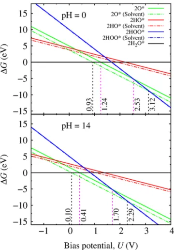
InFigure 4we show the free energy changeΔGfor different surface terminations as a function of bias potentialUat pH = 0 and pH = 14. We report results both for pure gas-phase conditions (solid lines) and in the presence of an implicit water environment (dotted lines). For small bias potentials, the most stable surface is H2O terminated, where molecular water is
adsorbed on surface Cd atoms at both pH values. The HOO terminated surface is stable above 3.12 V (2.53 V) bias potential with (without) implicit water at pH = 0, while in the range from 0.93 V (1.24 V) to 3.12 V (2.53 V) the O terminated surface is thermodynamically preferred under these conditions. Similar conclusions hold for pH = 14.
The inclusion of the solvent interaction results in a substantial shift of the relative stability with respect to the bias potentials. For example, the threshold bias for observing HOO terminated surface has increased by nearly 0.6 V by including the implicit solvent in the calculations.
6. CONCLUSIONS
A soft-sphere solvation model for ab initio electronic-structure calculations has been developed, parametrized, and tested. The transition from the dielectric cavity to outside is continuous and differentiable, allowing for the analytical calculation of the additional terms to the forces as well as the cavity-dependent nonelectrostatic contributions to the total energy that are described in terms of the quantum surface. As a consequence, we could obtain very high accuracy on energies and forces. The computational cost does not increase significantly with respect to standard gas-phase calculations. We expect that these features make our methods useful for numerous applications in material science. With fixed atomic radii, only two fitting parameters are needed to define the model, independently of the cluster or slab geometry. Mean absolute errors with respect to experimental solvation energies for neutral molecules and ions are close to the performances of others solvation approaches with a larger number of parameters. In particular for ions, the implemented approach outperforms in accuracy all
Table 5. Contributions to the Free Energy ChangeΔG
Computed at 298 K and 1 bar with Reference to the Standard Hydrogen Electrode for O, HO and HOO
Terminated CdS (112̅0) Surfacesa
ΔE[eV] ΔESolvent[eV] ΔEZPE[eV] TΔS[eV]
2O*(S) 6.39 5.14 −0.63 0.79
2HO*(Cd) 5.38 4.73 −0.40 0.56
2HOO*(Cd) 10.96 10.87 −0.82 0.10
aΔESolvent and ΔE are the change in energy calculated with and
without implicit solvent, respectively (eqs 25−27).
Figure 4.Free energy changeΔGas a function of the bias potentialU
for O, HO, HOO, and H2O terminated CdS (112̅0) surfaces at pH = 0
and pH = 14. Results obtained in pure gas-phase conditions (solid lines) and with the presence of an implicit water environment (dotted lines) are shown. Various threshold bias potentials are marked.
Journal of Chemical Theory and Computation