The effect of protective measures on risk-taking behavior and the moderating effect of sports: Testing the risk homeostatis theory by means of a computer game

(1)

0 Name: Gwyneth Wolfert

Student number: 1114476 Supervisor: Jop Groeneweg Second reader: William Verschuur Section: Cognitive Psychology

Master: Applied Cognitive Psychology

The effect of protective measures on risk-taking

behavior and the moderating effect of sports.

(2)

1

Abstract

This study investigates the risk homeostasis theory of Wilde (1982). This theory describes risk-taking behavior by addressing two levels of risk: the experienced risk level and the desired risk level. People are always trying to reach the desired risk level. Thus, if the experienced level of risk is below the desired level, people take compensatory actions (more risk-taking behavior) to reach the desired level. Additionally, the moderating effect of sports within risk homeostasis is studied. Studies have been done regarding the effect of sports on risk-taking in general, but no body of knowledge has been established on the moderating effect of sports in risk homeostasis. Based on the studies of sports on risk-taking in general, it is expected that there are some variables within sports and sportspeople that influence the moderating effect of sports on risk homeostasis. These are: intensity of sports, risk level of sports, position within sports and sporting style of the sportsperson.

A total of 69 participants were recruited. Participants were between 18 and 36 years old (M = 22,41, SD = 3,22). Data was gathered by means of two materials; a self-developed questionnaire and a computer game: the Spaceship game. The questionnaire focused on the sports-relevant information and the Spaceship game gathered the data needed for testing the risk homeostatic effect. In the game participants had to fly a spaceship through a galaxy while avoiding meteors. They received a certain amount of shields (representatively 0, 1, 3, 4 or 5) which represented their experienced risk level. During the game their speed, time to collision (TTC) and distance to closest meteor (DCM) were measured. It was hypothesized that an increase in protection (lower experienced level of risk) would lead to an increase in speed and a decrease in TTC and DCM, as participants would compensate for the low experienced risk level by showing more risk-taking behavior.

This study has found clear evidence for the risk homeostasis theory (Wilde, 1972). When the experienced level of risk was low, participants compensated this by showing more dangerous behavior in terms of speed, TTC and DCM. The moderating effect of sports shows interesting results. Sports participants show risk compensation, while non-sports participants do not. Also differences based on risk level, position and sporting style are found. Stronger risk compensation is reported in high(er) risk level sportspeople. Also sportspeople with a defensive position show stronger risk compensation than sportspeople with an offensive position. This also applies to sportspeople with a defensive sporting style versus sportspeople with an offensive sporting style.

(3)

2

Contents

List of tables and figures p. 4

1. Introduction p. 8

1.1 Risk homeostasis p. 8

1.1.1 Risk homeostasis: Support and critics p. 9

1.2 Risk homeostasis and sports p. 12

1.2.1 Intensity p. 13

1.2.2 Risk level p. 13

1.2.3 Position p. 14

1.2.4 Style p. 14

1.3 Present study p. 15

2. Methods p. 17

2.1 Participants p. 17

2.2 Materials p. 17

2.3 Design p. 19

2.4 Procedure p. 19

2.5 Analyses p. 19

3. Results p. 21

3.1 Hypothesis 1: Risk homeostasis p. 21

3.1.1 Between comparisons p. 21

(4)

3 3.8 Hypothesis 4B: Position within sports and risk homeostasis p. 57

3.9 Hypothesis 5A: Sporting style and risk-taking behavior p. 64 3.10 Hypothesis 5B: Sporting style and risk homeostasis p. 65

4. Discussion p. 72

4.1 Hypothesis 1 p. 72

4.2 Hypotheses 2A and 2B p. 72

4.6 Conclusion p. 76

4.7 Limitations p. 76

4.8 Future directions p. 78

References p. 79

Appendices p. 83

A. The questionnaire

B. Calculating the risk parameters C. Information letter

D. Informed consent

E. Instructions of the Spaceship game F. Debriefing

(5)

4

List of tables and figures

Tables

Table 1. Multivariate tests between conditions – Speed p. 21 Table 2. Descriptive statistics between conditions – Speed p. 22 Table 3. Multivariate tests between conditions – TTC p. 23 Table 4. Descriptive statistics between conditions – TTC p. 23 Table 5. Multivariate tests between conditions – DCM p. 24 Table 6. Descriptive statistics between conditions – DCM p. 24 Table 7. Multivariate tests within 1 shield condition – Speed p. 26 Table 8. Descriptive statistics within 1 shield condition – Speed p. 26 Table 9. Multivariate tests within 3 shields condition – Speed p. 27 Table 10. Descriptive statistics within 3 shields condition – Speed p. 27 Table 11. Multivariate tests within 3 shields condition – TTC p. 28 Table 12. Descriptive statistics within 3 shields condition – TTC p. 28 Table 13. Multivariate tests within 3 shields condition – DCM p. 28 Table 14. Descriptive statistics within 3 shields condition – DCM p. 28 Table 15. Multivariate tests within 4 shields condition – Speed p. 29 Table 16. Descriptive statistics within 4 shields condition – Speed p. 29 Table 17. Multivariate tests within 4 shields condition – TTC p. 30 Table 18. Descriptive statistics within 4 shields condition – TTC p. 30 Table 19. Multivariate tests within 4 shields condition – DCM p. 31 Table 20. Descriptive statistics within 4 shields condition – DCM p.31 Table 21. Multivariate tests within 5 shields condition – Speed p. 32 Table 22. Descriptive statistics within 5 shields condition – Speed p. 32 Table 23. Multivariate tests within 5 shields condition – TTC p. 33 Table 24. Descriptive statistics within 5 shields condition – DCM p. 33 Table 25. Multivariate tests within 5 shields condition – DCM p. 33 Table 26. Descriptive statistics within 5 shields condition – DCM p.34 Table 27. Descriptive statistics for Speed, TTC and DCM for the p. 37

independent variable hours of sport.

Table 28. Contrasts for speed on the different groups for hours of sport p. 37 Table 29. Descriptive statistics for speed for the independent variable p. 40

(6)

5 Table 30. Multivariate tests non-sports participants – Speed p. 42

Table 31. Multivariate tests sports participants – Speed p. 42 Table 32. Descriptive statistics for TTC for the independent variable p. 42

non-sports participants versus sports participants.

Table 33. Multivariate tests non-sports participants – TTC p. 43 Table 34. Multivariate tests sports participants – TTC p. 44 Table 35. Descriptive statistics for DCM for the independent variable p. 44

non-sports participants versus sports participants

Table 36. Multivariate tests non-sports participants – DCM p. 45 Table 37. Multivariate tests sports participants – DCM p. 46 Table 38. Descriptive statistics for Speed, TTC and DCM for the p. 47

independent variable risk level.

Table 39. Descriptive statistics for speed for the independent variable risk level (1) p. 48 Table 40. Descriptive statistics for speed for the independent variable risk level (2) p. 48

Table 41. Multivariate tests low risk – Speed p. 50

Table 42. Multivariate tests medium risk – Speed p. 50

Table 43. Multivariate tests high risk – Speed p. 50

Table 44. Descriptive statistics for TTC for the independent variable risk level (1) p. 51 Table 45. Descriptive statistics for TTC for the independent variable risk level (2) p. 51

Table 46. Multivariate tests low risk – TTC p. 52

Table 47. Multivariate tests medium risk – TTC p. 52

Table 48. Multivariate tests high risk – TTC p. 53

Table 49. Descriptive statistics for DCM for the independent variable risk level (1) p. 53 Table 50. Descriptive statistics for DCM for the independent variable risk level (2) p. 53

Table 51. Multivariate tests low risk – DCM p. 54

Table 52. Multivariate tests medium risk – DCM p. 54

Table 53. Multivariate tests high risk – DCM p. 55

Table 54. Descriptive statistics for Speed, TTC and DCM for the p. 56 independent variable position

Table 55. Descriptive statistics for speed for the independent variable position p. 57

Table 56. Multivariate tests defensive – Speed p. 58

Table 57. Multivariate tests offensive – Speed p. 59

Table 58. Descriptive statistics for TTC for the independent variable position p. 59

(7)

6

Table 60. Multivariate tests offensive – TTC p. 61

Table 61. Descriptive statistics for DCM for the independent variable position p. 61

Table 62. Multivariate tests defensive – DCM p. 62

Table 63. Multivariate tests offensive – DCM p. 63

Table 64. Descriptive statistics for Speed, TTC and DCM for the p. 64 independent variable sporting style

Table 65. Descriptive statistics for speed for the independent variable sporting style p. 65

Table 66. Multivariate tests more defensive – Speed p. 67

Table 67. Multivariate tests more offensive – Speed p. 67 Table 68. Descriptive statistics for TTC for the independent variable sporting style p. 67

Table 69. Multivariate tests more defensive – TTC p. 69

Table 70. Multivariate tests more offensive – TTC p. 69

Table 71. Descriptive statistics for DCM for the independent variable sporting style p. 69

Table 72. Multivariate tests more defensive – DCM p. 70

Table 73. Multivariate tests more offensive – DCM p. 71

Figures

Figure 1. Risk homeostatic model on driving behavior (Wilde, 1982) p. 8

Figure 2. Hypothesis 1 p. 16

Figure 3. Hypotheses 2a, 3a, 4a and 5a p. 16

Figure 4. Hypotheses 2b, 3b, 4b and 5b p. 16

Figure 5. Screenshot of the Spaceship game p. 18

Figure 6. Means plot for speed in the different conditions p. 22 Figure 7. Means plot for TTC in the different conditions p. 23 Figure 8. Means plot for DCM in the different condition p. 25 Figure 9. Means plot within 1 shield condition – Speed p. 26 Figure 10. Means plot within 3 shields condition – Speed p. 27 Figure 11. Means plot within 4 shields condition – Speed p. 30 Figure 12. Means plot within 5 shields condition – Speed p. 32

Figure 13. Means plot hours of sport – Speed p. 38

Figure 14. Means plot hours of sport – TTC p. 39

Figure 15. Means plot hours of sport – DCM p. 39

(8)

7 Figure 18. Means plot different groups hours of sport – DCM p. 45

(9)

8

1. Introduction

1.1 Risk homeostasis

This study will investigate the risk homeostasis theory (RHT) of Wilde (1982); a theory that describes risk-taking behavior. According to Wilde (1982), there are two different levels of risk: the experienced risk level and the desired risk level. People are always looking for an optimal level of risk and try to reach this desired risk level. If the experienced level of risk in one’s environment is below the desired level, people tend to take compensatory actions to reach this level, by participating in more risky behavior. So, people adapt their behavior to changes in the environment (Wilde, 1982). The risk homeostasis theory has been particularly studied in the field of traffic (e.g. Wilde, Robertson & Pless, 2002; Wilde, 1998; Aschenbrenner & Biehl, 1994; Jackson & Blackman, 1994; Grant & Smiley, 1993). It proposes that the implementation of preventive interventions (safety measures), for example ABS in cars, will automatically lower people’s perceived risk. This lower level of perceived risk in turn leads to more increased risky behavior (Wilde et al., 2002). Safety measures may therefore have contradictory effects and lead to more risky behavior and more accidents, while they are meant to reduce accidents.

Wilde (1982) compares the risk homeostatic effect within driver behavior with a thermostat (Figure 1). A thermostat always has a set point; the desired temperature, which in this case represents the desired risk level (target level). However, it might be cooler or hotter than this set point; the perceived temperature, which represents the perceived level of risk. Whenever there is a difference between the set point and the perceived temperature, a thermostat will take measures and starts heating or cooling in order to reach the desired temperature.

(10)

9 The desired level of temperature can differ per person and per context. So does the desired level of risk (Wilde, 1982). Based on a costs and benefits analysis people determine their desired level of risk. Four factors can be identified in this cost and benefits analysis:

1. The expected benefits of risk-taking behavior. 2. The expected costs of risk-taking behavior. 3. The expected benefits of safe behavior. 4. The expected costs of safe behavior.

When the expected benefits of risk-taking behavior and the expected costs of safe behavior are high, while the other two are low, it is to be expected that someone will show risk-taking behavior. However, if the perceived level of risk is already high people do not have to compensate, as there is a small difference or no difference at all between the perceived level and desired level of risk (Wilde, 1982).

If there is a significant difference between these two, people will start to adjust their behavior either by taking more risk or by taking less risk. This adjustment in behavior is influenced by two factors: (1) decision making skills and (2) vehicle handling skills. Eventually this will result in certain accident rates. This will influence the perceived level of risk of people. However, this might take some time as accident rates are not immediately available (lagged feedback). If the perceived level of risk changes, so does the set point of the ‘thermostat’; which will result in safer or more risk-taking behavior (Wilde et al., 2002).

Wilde (1982) assumes that lowering the willingness to take risks among people is the only solution to lower the number of accidents. Therefore the target level of risk has to be influenced. Wilde et al. (2002) considers rewards and punishments as the most promising solution for reducing the target level of risk. For instance, rewarding drivers that have driven ‘accident-free’ by giving them a bonus and punishing risk-taking behavior by high fines.

1.1.1 Risk homeostasis: Support and critics

The risk homeostasis theory has been studied extensively. Supporting evidence as well as opposing evidence can be found in research. Both will be discussed below.

(11)

10 drivers were used to the right-hand driving and the accidents rates were back to normal; the perceived level of risk was decreased and drivers compensated this by showing more risk-taking behavior (Wilde et al., 2002; Wilde, 1998). Additional support from real-life examples is provided by Aschenbrenner & Biehl (1994). They studied taxi drivers in Munich who received a cab equipped with anti-lock brakes (ABS). Their behavior changed once this safety measure was added: they showed more risk-taking behavior, thereby keeping the accident rates with cabs constant over time (Aschenbrenner & Biehl, 1994). The same evidence was found in Canada by Grant & Smiley (1993). One of the specific results was that the taxi drivers who had ABS slightly increased their speed.

Besides real-life studies, several researches have also been conducted in simulated environments. Jackson and Blackman (1994) introduced rewards and punishments as motivators for decreasing risk-taking behavior, thereby changing the desired level of risk. Results showed that an increase in costs of risk-taking behavior resulted in a decrease of accidents (Jackson & Blackman, 1994). Hoyes, Stanton and Taylor (1996) also conducted a driving simulator test. Their experiment manipulated the experienced level of risk: participants were exposed to environments with high risk and low risk. Results showed that less accidents occurred in the high risk environment (Hoyes et al., 1996). Due to a higher level of perceived risk, risk-taking behavior compensation was not needed. This resulted in safer behavior. Glendon, Hoyes, Haigney & Taylor (1996) also reviewed the risk homeostasis theory and found support for the theory, but also found that risk compensation can occur in very short-term time. This contradicts the risk homeostasis theory which states that risk compensation sometimes takes months or even years. This result might be explained by the immediate feedback of simulators on participants (Glendon et al., 1996; Hoyes et al., 1996).

(12)

11 use them at all (Maughan-Brown & Venkataramani, 2012). Some researchers have also applied the risk homeostasis theory within work settings and found support for risk compensation (Sagan, 1997; Stetzer & Hofmann, 1996). At last, the effect of alcohol on gambling has been connected to the risk homeostasis theory (Breslin, Sobell, Capell & Vakili, 1999).

Besides supporting evidence for the risk homeostasis theory, there are also some critical findings. Evans (1986) used a wide variety of accident data to see whether he could support the theory. But all data that he researched was incompatible with the theory. He studied the reintroduction of a law in 1970 in some states in the United States. The law demanded motorcyclists to wear a helmet. According to the risk homeostasis theory this should lead to a lower rate of accidents shortly after the implementation and after a while the accident rates should be back to normal. The states that did not implement the law should have no changes in their accident rates. Data showed that the states that reintroduced the law had an increase of 28 percent in motorcyclist fatalities in comparison with the states that did not reintroduced the law (Evans, 1986). Also Evans (1986) questioned a more general assumption of the risk homeostasis theory; he found no evidence for the homeostatic effect that presumes that accident rates stay relatively stable over time.

Shannen and Szatmari (1994) have examined the injury rates before and after the introduction of seat-belt legislation in Britain. According to the risk homeostasis theory a difference would be expected as drivers with seat-belts would feel more protected and therefore would compensate showing more risk-taking behavior. Results indicated no (significant) differences in injury rates. However, it is not possible to determine what factors have influenced this. Evans (1986) addressed in his research the ‘selective recruitment issues’ with safety measures; safety measures may not decrease the number of accident rates due to the effect on a specific target group. For instance, the introduction of the mandatory seat belt law may not lead to decreases in accident rates because only safer drivers comply with this law.

Hoyes, Dorn, Desmond and Taylor (1996) tested the risk homeostasis theory in a simulated environment. The theory states that behavioral change only occurs when there is an utility to be gained. According to the theory intrinsic risk and utility should show a statistical interaction. Hoyes et al. (1996) found no support for this; data showed that participants took more risk when there was more at stake.

(13)

12 can be measured. Therefore if the number of accidents is reduced, the target level of risk must have changed. If the number of accidents has increased, the target level of risk must also have changed. If the numbers of accidents are stable, the target level of risk must have stayed equal. Therefore, the theory is always correct and cannot be falsified (Elvik, 2004; Glendon et al., 1996; Hoyes & Glendon, 1993; Adams, 1988). Glendon et al. (1996) do mention that a well-designed laboratory experiment might be able to control all the potential factors that influence homeostasis and therefore might be able to falsify (or support) the theory in a correct empirical way.

1.2 Risk homeostasis and sports

As said, the risk homeostasis theory has been applied in some other domains besides traffic. One of them being sports. In sports people are often exposed to (high) risks. Therefore, with many sports protective measures are taken, mostly by wearing specific kind of clothing, e.g. with rugby, ice-hockey, soccer and hockey. It seems to make perfect sense that this protective clothing enables sportspeople to take more risks. Research shows that wearing protective clothing does indeed give sportspeople more confidence, results in more risky behavior, and in turn, results in more accidents (Hagel & Meeuwisse, 2004; Stuart, Smith, Malo-Ortiguera et al., 2002; Finch, McIntosh, McCrory, 2001).

Napier, Findley and Self (2007) researched the effect of a safety measure in skydiving: the Cypres Automatic Activation Device (AAD). This device automatically opens the (reserve) parachute after a specific time. Logically, this device decreased the so-called no pull/low pull fatalities. However, there was an increase in so-called open canopy fatalities. The overall number of fatalities remained relatively stable (Napier, Findley & Self, 2007). Risk homeostasis has also been studied in skiing. Results show that 33 percent of all skiers and snowboarders reported to take more risk when wearing a helmet (Ruedl, Abart, Ledochowski, Burtscher & Kopp, 2012; Scott, Buller, Andersen et al., 2007). However, other research on alpine skiing did not show higher rates of accidents for those who wear a helmet (Ruedl, Brunner, Kopp & Burtscher, 2011; Hagel, Pless, Goulit, Platt & Robitaille, 2005).

(14)

13 (Farris, Spaite, Criss et al., 1997). Altogether, various researches have been conducted to test the risk homeostasis theory in sports. Until now it has resulted in contradictory results.

These contradictory results might be explained by the differences between different sport(s) and sportspeople. Depending on for instance risk level, it could be explained why risk homeostasis was found in skydiving and not in cycling; these sports attract different kind of sportspeople and these sportspeople might differ in their desired risk level (Zuckerman & Stelmack, 2004). As this study does not lend itself for real-life sport tests, the effect of risk homeostasis within (a certain) sport(s) cannot be measured. However, it is far more interesting to compare risk homeostasis within different sportspeople. This can be studied in any controlled environment. Two effects will be researched: First the effect of sports on risk-taking behavior in general will be measured. Second, the actual moderating effect of sports on risk homeostasis will be measured. Until now, the first effect has given a lot of controversial results, which will be described in the following paragraphs. For the second effect, no established body of knowledge exists yet. As risk-taking is a prominent part of the risk homeostasis theory, researching the first effect (sports on risk-taking) can give valuable insights regarding the second effect (moderating effect of sports on risk homeostasis) and will give a more complete picture of the risk-taking behavior of sportspeople.

For both effects, different groups of sportspeople will be identified to see whether there is a difference in their risk-taking behavior and their risk compensation strategy (risk homeostasis). These different groups of sportspeople will be categorized based on four different elements within their sports: intensity, risk level of sport, position and sporting style.

1.2.1 Intensity

Several studies have investigated the differences between sports participants versus non-sports participants on risk-taking behavior (outside the field). Garry & Morrissey (2000) found that sports participants in general show more risk-taking behavior than non-sports participants. Martha & Griffet (2007) however, found that sports participants report lower risk-taking and higher risk perception. Other research found mixed findings; both increases and decreases of risk-taking behavior in sports participants (Peck, Vida & Eccles, 2007). A possible explanation for these contradictory results might be that the intensity of participation in sports influences the effect. A sportsperson that practices 7 hours a week might be more prone to endure in his sport-related risk-taking behavior than a sportsperson that practices only 1 hour a week. Additionally, this effect might also endure in his or her risk compensation strategy.

1.2.2 Risk level

(15)

14 determined by means of the injury rate per 1000 hours (Zuckerman & Stelmack, 2004). Walking can for instance be classified as a low risk sport while indoor soccer can be classified as a high risk sport (TNO, 2015).

It is supported that depending on the sport, risk-taking behavior and risk compensation of the sportsperson differs both in the field, as well as outside the field (Zuckerman & Stelmack, 2004). Research shows that sportspeople who participate in high risk sports score far higher on sensation seeking than sportspeople participating in medium risk or low risk sports (Zuckerman & Stelmack, 2004). The mixed findings of the above mentioned researches (Martha & Griffet, 2007; Peck et al., 2007; Garry & Morrisey, 2000) may be explained by their lack of accounting the risk level of the sport(s) in their researches. Therefore, the risk level of sports will be also included and studied in this research. It is expected that depending on the risk level of sports, a sportsperson shows more of less risk-taking behavior outside the field and uses a different risk compensation strategy.

1.2.3 Position

Garry & Morrissey (2000) made an attempt to study the differences in risk-taking behavior between team sports participators vs. non-team sports participators. This resulted in no conclusive results and further research was advised as differences are expected based on positions played within a team sport (Garry & Morrissey, 2000). Some other studies have been conducted in the meanwhile regarding this topic. These studies were all conducted within the field, so no general effect of position on risk-taking was measured. Headrick et al. (2011) compared defenders, midfielders and forwards in soccer. The study showed that the distance to the goal has an effect on tactics and style of players. Players closer to the goal tend to have a bigger distance between themselves and the ball when dribbling, so a higher risk on losing the ball. This effect was especially strong for forwards. Defenders, even when they were close to the goal, kept the ball closer to themselves when dribbling (Headrick et al., 2011). A comparable study showed the same results for basketball players (Cordovil et al., 2009). These results support the fact that forwards show more risk-taking behavior as they have a larger distance between themselves and the ball and therefore a larger risk on losing the ball to the opponent. Whether this behavior also endures in other situations and has an effect on risk compensation will be researched as well.

1.2.4 Sporting style

(16)

15 determined by a subjective judgment of participants themselves. It will be researched whether sporting style has an effect on risk-taking behavior and risk compensation.

1.3 Present study

The goal of this study is to investigate whether the risk homeostasis theory is supported or falsified. The theory of Wilde (1982) is controversial. Different results have been found until know. This research will investigate this controversy and will gain more insights in the phenomenon of risk-taking behavior and the effects of safety measures and risk perception on risk-taking behavior. The dependent variable of this study will be risk-taking behavior and the independent variable will be the level of protection/safety. It is expected that higher levels of safety will lead to more risk-taking behavior as there is a bigger gap between the experienced risk level and the desired risk level.

This study will also examine the moderating effect of sports on risk homeostasis. There is no established body of knowledge yet on this subject. Therefore, the effect of sports on risk-taking behavior (without including the independent variable of protection/safety) will be measured first. Until now, many contradictive evidence exists. Gaining insight in the risk-taking behavior of participants can also give help to interpret their risk compensation strategy. With regard to these two effects it is expected that the intensity, risk level, position and sporting style influences the risk-taking behavior and risk compensation strategy of sportspeople.

The main research question of this study is: What is the effect of protective measures on risk-taking behavior (risk homeostasis) and what is the moderating effect of sports?

The following hypotheses will be tested:

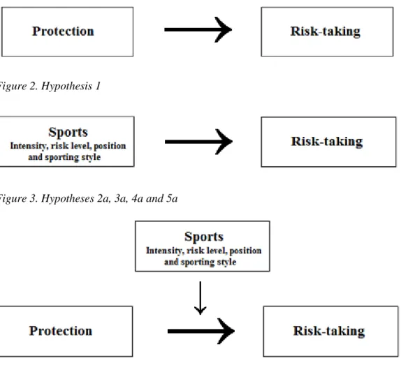
Hypothesis 1: Higher levels of protection will lead to more risk-taking behavior.

Hypothesis 2a: More participation in sports (in hours) leads to more risk-taking behavior.

Hypothesis 2b: Depending on the participation in sports (in hours), a different risk-compensation strategy can be expected within different groups of sportspeople.

Hypothesis 3a: Sportspeople who participate in high risk sports will show more risk-taking behavior, compared to sportspeople who participate in medium risk and low risk sports.

Hypothesis 3b: Depending on the risk level of the sport (low, medium or high), a different risk-compensation strategy can be expected within different groups of sportspeople

(17)

16 goalkeeper).

Hypothesis 4b: Depending on the position played within a sport (defensive versus offensive), a different risk-compensation strategy can be expected within different groups of sportspeople.

Hypothesis 5a: Sportspeople who perceive their sporting style as more offensive show more risk-taking behavior than sportspeople who perceive their sporting style as more defensive.

Hypothesis 5b: Depending on the perceived sporting style (more defensive versus more offensive), a different risk-compensation strategy can be expected within different groups of sportspeople.

This research will result in valuable new scientific insights. Both the risk homeostasis theory as well as the effect of sports on risk-taking have resulted until now in contradictory results. Besides new scientific knowledge, this research is also socially relevant as protective measures are often implemented in society to reduce accidents. If evidence is found for the possible negative effects of protective measures, this can have big societal changes regarding safety measures.

Figure 2. Hypothesis 1

Figure 3. Hypotheses 2a, 3a, 4a and 5a

(18)

17

2. Methods

2.1 Participants

For the present study, a group of 69 participants was recruited. Participants were between 18 and 36 years old (M = 22,41, SD = 3,22). The majority of the participants were female; 58 compared to 11 males. Participants’ highest completed education level varied from higher general secondary education to postgraduates. Most participants either completed pre-university secondary education (N = 33) or were undergraduate (N = 23).

Participants were recruited by means of Sona; the Leiden University research participation program. An advertisement was placed and a total of 62 students subscribed of whom 51 showed up. The other 18 participants were recruited within the social environment of the researchers and by means of distributing flyers at the faculty of social sciences.

Exclusion criteria of the study was the presence of a neurological condition or experience in the past with the Spaceship game. During the study as well as afterwards, no technical problems occurred. All data was complete. This resulted in a final sample of 69 participants.

2.2 Materials

Data was gathered by means of two materials; a self-developed questionnaire and a computer game: the Spaceship game. The questionnaire was made by use of the Online Survey Software Qualtrics. It consisted out of one general question, three demographic questions and six sport-related questions (see Appendix A). All questions were in English. This questionnaire was used as an instrument to gather all relevant information about participation in sports. The questionnaire was filled out on the computer.

(19)

18

Figure 5. Screenshot of the Spaceship game.

The game consisted out of a preview, in which participants watched a short example of the game. Subsequently they started with a test round, in which they were randomly assigned 0 or 3 shields. After that, participants played five rounds in which they were assigned in random order 0, 1, 3, 4 and 5 shields. This variety in number of shields represented the perceived level of risk. A high number of shields represented a low level of risk and a low number of shields represented a high level of risk. As soon as all protection shields were lost a new session started. A maximum duration of four minutes was set for each session. Those who had managed to navigate through the galaxy without losing all shields were automatically stopped after four minutes.

(20)

19

2.3 Design

The experiment had five within-subject conditions; the five different sessions. These conditions each had a different amount of protection shields; 0, 1, 3, 4 or 5. In total every participant received 13 protection shields. The shields were assigned in a random order to the participant. Both the participant as well as the researchers did not know the order of the assigned protection shields. The experiment can be defined as a double-blind randomized design with five within-subject conditions.

2.4 Procedure

The experiments were conducted in one of the computer rooms at the Faculty of social sciences, Wassenaarseweg 52 in Leiden. The computers all had a 21 inch display. The study was conducted in four testing days. Each day at least two researchers were present. The experiment lasted around 45 minutes, depending on the working speed of the participant.

Upon arrival, all participants were given an information letter and an informed consent (Appendices C and D). The information letter gave general information about what the participants were going to do and reassured the participant that all data was coded in an anonymous way. Also participants were informed that their participation was voluntarily and that they could stop whenever they want. After reading the information letter and signing the informed consent, the Spaceship game was put on by one of the researchers. The spaceship itself contained detailed instructions for participants on how to navigate the spaceship (See Appendix E). They were also instructed that they would gain points during the game. However, these were invisible to the participants. The points they gained depended on the difficulty level and the total ‘flying’ time. The three best players were granted a prize (50, 30 and 10 euros). At the end of the game they were instructed to raise their hand so the questionnaire could be put on. After completing the questionnaire participants could come and collect their credits or money (2 credits or 6,50 euros). They also got a debriefing letter (Appendix F) with more specific information about the research. A week after the experiments the winning participant numbers were announced by e-mail.

2.5 Analyses

(21)

20 hours of sport. This classification was made by use of the statistics from the annual OBiN (Ongevallen en Bewegen in Nederland) questionnaires from 2000 till 2014 (TNO, 2015). Participants that did not participate in a sport were not included in the analysis of hypothesis 3a and 3b. The risk level of the participants that participated in more than one sport was defined by their ‘main sport’ (the sport they spend most hours per week on). If this was equal for two (or more) sports, the main sport was defined by their years of experience. Variable 3 was computed as a categorical variable with 2 categories: defensive (which includes goalkeeper, defender and defensive midfielder) and offensive (which includes offensive midfielder and forward). Variable 4 was also computed as a categorical variable with 2 categories: more offensive and more defensive. The last two variables included the option ‘not applicable’ in the questionnaire. Participants that selected this option were not included in the analyses.

The data from the videogame was registered each millisecond in the file ‘steplog’. Several parameters were registered: participant number, number of the session, time, score (points), level of difficulty, amount of shields, the position of the spaceship on the y-axis, the meteor closest to the spaceship on both the y-axis and the x-axis and the collisions. The same parameters were registered in the file ‘eventlog’ at the specific moments of collision. The data from steplog was used to calculate three risk parameters: speed, time to collision (TTC) and distance kept to the closest meteor (DCM) (See Appendix B).

To test hypothesis 1 several repeated measures ANOVA’s were conducted. This test automatically corrects for cumulative type-1 errors and is therefore more reliable than conducting multiple paired sampled t-tests. The repeated measures ANOVA’s tested whether there were significant differences in the means (speed, TTC and DCM) between the conditions and within the conditions. Before starting the analysis for hypothesis 1, assumptions for the repeated measures ANOVA were checked. These can be found in the results section.

For hypothesis 2a, 3a, 4a and 5a (effect of different elements of sports on risk-taking behavior) a MANOVA was initially planned to use. The assumptions for this test were checked beforehand, resulting in many limitations. Therefore the hypotheses were tested using three separate ANOVA’s; one for speed, one for TTC and one for DCM. Reports on the assumption checks for MANOVA can also be found in the results section.

(22)

21

3. Results

3.1 Hypothesis 1: Higher levels of protection will lead to more risk-taking behavior.

Assumptions repeated measures ANOVA

The dependent variables (speed, TTC and DCM) are all measured on a continuous scale. Furthermore, the within-subjects factor is categorical with two or more levels. The third assumption, no significant outliers in any level of the within-subjects factor, were tested using boxplots. Outliers were found but these were not removed as they are all related to the phenomenon that is being researched.

The fifth assumption, a normal distribution for the dependent variables for each level of the within-subjects factor, was measured using the normal Q-Q plots. Shapiro Wilks test was not consulted due to the reduced reliability in large sample sizes (N > 50). All normal Q-Q plots showed a normal distribution of the dependent variables. The sixth assumption, the assumption of sphericity, will be checked during the analysis.

3.1.1 Between comparison

Speed

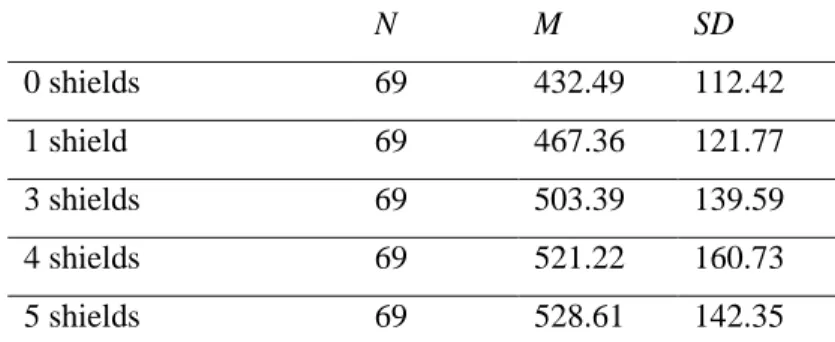
Mauchly’s test indicated that the assumption of sphericity was met, X2(9), = 11.508, p = .243. The multivariate tests were all significant (p < .001) and the univariate result also shows that there is a significant difference in mean speed between the different conditions, F(4, 272) = 17.44, p < .001. Therefore, post-hoc bonferroni corrected pairwise comparisons were conducted. The pairwise comparisons showed significant differences between the condition with 0 shields and the conditions with 3 shields (p < .001), the condition with 0 shields and the condition with 4 shields (p < .001) and the condition with 0 shields and the conditions with 5 shields (p < .001). Two other significant effects were found between the condition with 1 shield and the condition with 4 shields (p = .005) and the condition with 1 shield and the condition with 5 shields (p < .001). Figure 6 shows that the significant effects indicate an increase in speed is related to an increase in lives.

Value F p

Pillai’s Trace .445 13.045 .000

Wilks’ Lambda .555 13.045 .000

Hotelling’s Trace .803 13.045 .000 Roy’s Largest Root .803 13.045 .000

(23)

22

N M SD

0 shields 69 432.49 112.42

1 shield 69 467.36 121.77

3 shields 69 503.39 139.59

4 shields 69 521.22 160.73

5 shields 69 528.61 142.35

Table 2. Descriptive statistics between conditions – Speed

Figure 6. Means plot for speed in the different conditions

TTC

(24)

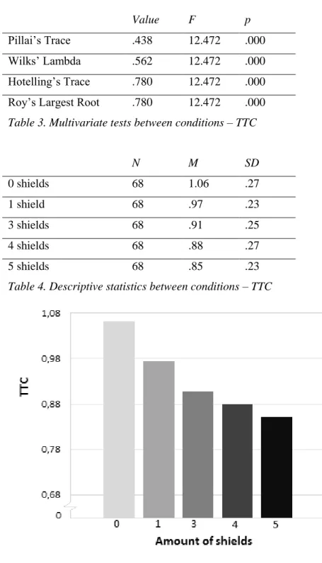
23 (p = .012) and the condition with 1 shield and the condition with 5 shields (p < .001). The graph below shows that the significant effects indicate an decrease in TTC is related to an increase in lives.

Value F p

Pillai’s Trace .438 12.472 .000

Wilks’ Lambda .562 12.472 .000

Table 3. Multivariate tests between conditions – TTC

N M SD

0 shields 68 1.06 .27

1 shield 68 .97 .23

3 shields 68 .91 .25

4 shields 68 .88 .27

5 shields 68 .85 .23

Table 4. Descriptive statistics between conditions – TTC

(25)

24

DCM

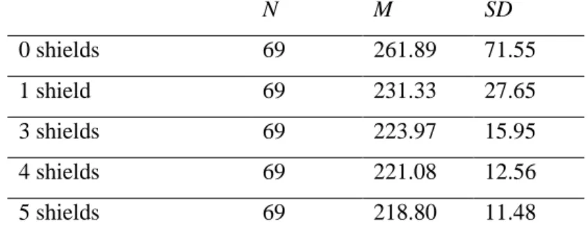
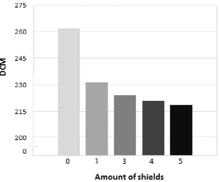
All multivariate tests were significant, p < .001. Mauchly’s test indicated that the assumption of sphericity was not met, X2(9), = 321.123, p < .001. Therefore, degrees of freedom were corrected by using the Greenhouse-Geisser estimates of sphericity (ε = .336). The results show that there is a significant difference in mean DCM between the different conditions, F(1.345, 91.462) = 21.662, p < .001. Therefore, post-hoc bonferroni corrected pairwise comparisons were conducted. The pairwise comparisons showed significant differences between the condition with 0 shields and the condition with 1 shield (p = .002), the condition with 0 shields and the condition with 3 shields (p < .001), the condition with 0 shields and the condition with 4 shields (p < .001) and the condition with 0 shields and the condition with 5 shields (p < .001). Three other significant effects were found between the condition with 1 shield and the condition with 4 shields (p = .011), the condition with 1 shield and the condition with 5 shields (p = .001) and the condition with 3 shields and the condition with 5 shields (p = .023). The graph below shows that the significant effects indicate an decrease in DCM is related to an increase in lives.

Value F p

Pillai’s Trace .318 9.996 .000

Wilks’ Lambda .619 9.996 .000

Table 5. Multivariate tests between conditions – DCM

N M SD

0 shields 69 261.89 71.55

1 shield 69 231.33 27.65

3 shields 69 223.97 15.95

4 shields 69 221.08 12.56

5 shields 69 218.80 11.48

(26)

25

Figure 8. Means plot for DCM in all conditions

3.1.2 Within comparisons – One shield condition

Repeated measure ANOVA’s were also conducted within each condition to see whether the decrease in lives during one session causes risk homeostasis. For TTC and DCM the first shield of every condition was left out as this data was clouded. The formula used to measure these risk parameters uses the distance to meteorites. However, at the very beginning of the game the meteorites still have to ‘fly in’ on the screen. Therefore, the TTC and DCM of the first shields are not reliable and may not be included in the within comparisons. Overall, this means that the one shield condition only includes speed. The condition of zero shields is not included as there is no comparison to make with other shields.

Speed

(27)

26

Value F p

Pillai’s Trace .433 51.994 .000

Wilks’ Lambda .567 51.994 .000

Table 7. Multivariate tests within 1 shield condition – Speed

N M SD

1/1 shields 69 440.20 110.43

0/1 shields 69 524.69 164.87

Table 8. Descriptive statistics within 1 shield condition – Speed

Figure 9. Means plot within 1 shield condition – Speed

3.1.3 Within comparisons – Three shields conditions

Speed

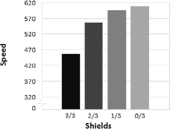
The multivariate approach shows that all tests are significant, p < .001 (Table 9). Mauchly’s test indicated that the assumption of sphericity was not met, X2(5), = 62.85, p < .001. Therefore, degrees of freedom were corrected by using the Greenhouse-Geisser estimates of sphericity (ε = .611). The results show that there is a significant difference in mean speed within the three shield condition, F(1.83, 104.61) = 49.58,

(28)

27 .001) and 2 shields left and 0 shields left (p = .001). There was no significant effect between 1 shield left and 0 shields left (p = 1.000).

Value F p

Wilks’ Lambda .761 8.774 .000

Table 9. Multivariate tests within 3 shields condition – Speed

N M SD

3/3 shields 58 458.06 113.27

2/3 shields 58 556.83 171.11

1/3 shields 58 596.79 185.98

0 shields 58 608.20 179.44

Table 10. Descriptive statistics within 3 shields condition – Speed

Figure 10. Means plot within 3 shields condition – Speed

TTC

(29)

28 condition, F(2, 114) = 2.239, p = .111. Therefore, no post-hoc tests were executed. Differences were too small to graphically display.

Value F p

Wilks’ Lambda .929 2.148 .126

Table 11. Multivariate tests within 3 shields condition – TTC

N M SD

2/3 shields 58 .75 .34

1/3 shields 58 .68 .31

0/3 shields 58 .69 .29

Table 12. Descriptive statistics within 3 shields condition – TTC

DCM

Mauchly’s test indicated that the assumption of sphericity was met, X2(2), = 2.874, p = .238. Both the multivariate approach (p = .640) and the univariate approach showed no significant results, F (2, 114) = 0.362, p = .697. Therefore, no post-hoc tests were executed. Differences were too small to graphically display.

Value F p

Pillai’s Trace .016 .450 .640

Wilks’ Lambda .984 .450 .640

Hotelling’s Trace .016 .450 .640 Roy’s Largest Root .016 .450 .640

Table 13. Multivariate tests within 3 shields condition – DCM

N M SD

2/3 shields 58 203.31 16.43

1/3 shields 58 202.83 16.21

0 shields 58 205.08 12.37

(30)

29

3.1.4 Within comparisons: Four shields condition

Speed

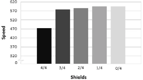
The multivariate approach shows significant results, p < .001 (Table 15). Mauchly’s test indicated that the assumption of sphericity was not met, X2(9), = 113, p < .001. Therefore, degrees of freedom were corrected by using the Greenhouse-Geisser estimates of sphericity (ε = .515). The univariate results show that there is a significant difference in mean speed within the four shield condition, F(2.059, 115.31) = 36.817, p < .001. Post-hoc Bonferroni-corrected pairwise comparisons showed significant differences between 4 shields left and all three other shield conditions (all p < .001). No other significant effects were found.

Value F p

Pillai’s Trace .566 17.276 .000

Wilks’ Lambda .434 17.276 .000

Hotelling’s Trace 1.304 17.276 .000 Roy’s Largest Root 1.304 17.276 .000

N M SD

4/4 shields 57 473.79 142.83

3/4 shields 57 578.07 195.87

2/4 shields 57 586.18 178.60

1/4 shields 57 594.91 184.60

0/4 shields 57 595.49 183.13

(31)

30

TTC

Multivariate tests show no significant results, p =.816 (Table 16). Mauchly’s test indicated that the assumption of sphericity was not met, X2(5), = 16.53, p = .005. Therefore, degrees of freedom were corrected by using the Huynh-Feldt estimates of sphericity (ε = .838). The univariate results also show that there is no significant difference in mean TTC within the four shield condition, F (2.642, 147.965) = 0.231, p = .852. Therefore, no post-hoc tests were executed. Differences were too small to graphically display.

Value F p

Wilks’ Lambda .983 .313 .816

N M SD

3/4 shields 57 .74 .28

2/4 shields 57 .73 .29

1/4 shields 57 .71 .27

0/4 shields 57 .73 .27

(32)

31

DCM

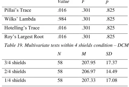
Multivariate tests show no significant results, p = .825 (Table 19). Mauchly’s test indicated that the assumption of sphericity was met, X2(5), = 4.149, p = .528. The univerariate results show also that there is no significant difference in mean DCM within the four shield condition, F(3, 171) = 0.263, p = .852. Therefore, no post-hoc tests were executed. Differences were too small to graphically display.

Value F p

Wilks’ Lambda .984 .301 .825

Table 19. Multivariate tests within 4 shields condition – DCM

N M SD

3/4 shields 58 207.95 17.37

2/4 shields 58 206.97 14.49

1/4 shields 58 207.33 17.08

0/4 shields 58 209.24 14.52

Table 20. Descriptive statistics within 4 shields condition – DCM

3.1.5 Within comparisons: Five shields condition

Speed

(33)

32

Value F p

Pillai’s Trace .556 14.500 .000

Wilks’ Lambda .444 14.500 .000

N M SD

5/5 63 456.74 119.29

4/5 shields 63 555.47 172.89

3/5 shields 63 576.11 183.92

2/5 shields 63 585.34 181.86

1/5 shields 63 590.94 172.34

0/5 shields 63 592.98 184.65

Table 22. Descriptive statistics within 5 shields condition – Speed

TTC

(34)

33 significant difference in mean TTC within the five shield condition, F(3.317, 205.666) = 4.23, p = .005. Therefore, post-hoc bonferroni corrected pairwise comparisons were conducted. The pairwise comparisons showed significant differences between 4 shields left and 2 shields left (p = .011), 4 shields left and 1 shield left (p = .038) and 4 shields left and 0 shields left (p = .02). Differences were too small to graphically display.

Value F p

Wilks’ Lambda .786 4.027 .006

N M SD

4/5 shields 63 .79 .28

3/5 shields 63 .74 .28

2/5 shields 63 .73 .27

1/5 shields 63 .71 .24

0/5 shields 63 .70 .28

Table 24. Descriptive statistics within 5 shields condition – TTC

DCM

Multivariate tests show no significant effects, p = .812 (Table 25). Mauchly’s test indicated that the assumption of sphericity was met, X2(9), = 16.274, p = .061. The univariate results also show that there is no significant difference in mean DCM within the five shield condition, F(4, 248) = 0.455, p = .768. Therefore, no post-hoc tests were executed. Differences were too small to graphically display

Value F p

Wilks’ Lambda .974 .394 .812

(35)

34

N M SD

4/5 shields 63 207.89 13.90

3/5 shields 63 205.25 18.84

2/5 shields 63 207.48 12.93

1/5 shields 63 205.43 14.42

0/5 shields 63 205.65 17.47

(36)

35

3.2 Preparatory analyses risk-taking and risk homeostasis hypotheses

MANOVA

Before the MANOVA’s were conducted for the hypotheses 2a, 3a, 4a and 5a, assumptions were checked. The dependent variables (speed, TTC and DCM) are all on interval or ratio level. The independent variables (sport in hours, risk level sport, objective position and subjective position) are all categorical and have two or more independent groups. Furthermore, there is independence of observations and there is an adequate sample size; in each group of the independent variables there are more cases than the number of dependent variables (>3).

Univariate outliers and multivariate outliers were not identified as these are related to the phenomenon that is being researched.

Next, multivariate normality was tested. SPSS does not offer a test for multivariate normality, therefore multiple normality tests (Shapiro-Wilks) had to be performed. Normality of each of the dependent variables for each group of the independent variable was tested. Almost all Shapiro-Wilks tests were not significant, indicating normality of the data. Only one Shapiro-Wilks test was significant: the mean of DCM in the ‘more defensive’ group (variable 4, hypothesis 3b), p = .005. Multiple transformations of the mean of DCM resulted in no changes regarding normality. The one-way MANOVA is fairly robust to deviations of normality. Therefore, the mean of DCM was included in the analyses. The non-normality will be taken into account when reporting the results. .

Multicollinearity was tested by calculating the correlations between the three dependent variables. The tests show that Speed and TTC are highly (negatively) correlated with each other (r = -.957, p < .001), while speed and DCM are not correlated at all (r = 0.06, p = .638). Also TTC and DCM are not correlated (r = -.016, p = .897). Therefore, speed was taken out of the MANOVA. The effect of the independent variables on speed will be independently calculated by an separate ANOVA.

Homogeneity of variance-covariance matrices was tested using Box’s M test of equality of covariance. For the first variable (hours of sport) there was homogeneity of variance-covariances matrices, as assessed by Box’s test of equality of covariance matrices (p = .844). Also the second variable (risk level of sport) showed homogeneity of variance-covariance matrices (p = .509), as well as the other two variables (position: p = .388 and style: p = .926). The assumption of homogeneity of variance-covariance matrices is met.

(37)

36 was no clear linear relationship between DCM and TTC for each group of the independent variable. Also the linear relationship between speed and DCM was checked (In case there would be a linear relationship, TTC could be excluded from the MANOVA instead of speed). However, there was also no linear relationship between speed and DCM. Multiple transformations, both for DCM, TTC and speed did not result in a linear relationship.

Due to the violation of the linearity assumption the two dependent variables were separated from each other; resulting in three separate ANOVA’s to test each of the hypotheses. As the assumptions for MANOVA also include most assumptions of a one-way ANOVA, no additional preparatory analyses have to be conducted. The homogeneity of variances, using Levene’s test, will be checked during the analysis.

Repeated measures ANOVA

Hypotheses 2b, 3b, 4b and 5b were tested using repeated measures ANOVA’s. The dependent variables (speed, TTC and DCM) are all measured on a continuous scale. Furthermore, the within-subjects factor is categorical with two or more levels. The third assumption, no significant outliers in any level of the within-subjects factor, were tested using boxplots. Outliers were found but these were not removed as they are all related to the phenomenon that is being researched.

(38)

37

3.3 Hypothesis 2a: More participation in sports (in hours) leads to more risk-taking behavior.

An one-way ANOVA was conducted with the mean of speed as dependent variable and the hours of sport as the independent variable. Two other one-way ANOVA’s were conducted with the mean of TTC and the mean of DCM as dependent variables. The means and standard deviations of these dependent variables for each group of the independent variable can be found in Table 27.

Speed TTC DCM

N M SD M SD M SD

0 hours 11 457.15 92.61 .99 .16 217.33 6.28

0-1 hours 10 468.26 112.98 .97 .24 221.02 5.94

1-2 hours 7 511.97 128.08 .90 .22 216.53 6.22

2-3 hours 15 544.33 129.44 .85 .20 227.63 23.30

3-4 hours 7 444.09 76.27 1.15 .19 220.02 8.61

4-6 hours 9 527.28 81.96 1.02 .18 220.80 8.00

> 6 hours 10 485.58 102.53 .87 .13 221.97 9.78

Table 27. Descriptive statistics for Speed, TTC and DCM for the independent variable hours of sport.

Speed

The assumption of homogeneity of variances was met, as assessed by Levene’s test for equality of variances (p = .388). The mean speed was significantly different for the different groups on the independent variable, F(6, 62) = 2.262, p = .049. As the hypothesis implies a specific difference between the groups of the independent variables (more participation in sports is accompanied by more speed), post-hoc Tuckey’s test are not suitable. Instead, custom contrasts were ran to see whether support was found for the hypothesis. Six different contrasts were entered in SPSS, these can be found in table 28. Bonferroni-corrected alpha levels of .00833 were used (.05/6).

Contrast 0 hours 0-1 hours 1-2 hours 2-3 hours 3-4 hours 4-6 hours > 6 hours

1 -1 1 0 0 0 0 0

2 0 -1 1 0 0 0 0

3 0 0 -1 1 0 0 0

4 0 0 0 -1 1 0 0

5 0 0 0 0 -1 1 0

6 0 0 0 0 0 -1 1

(39)

38 Results showed that only the fourth contrast, 2-3 hours sports a week versus 3-4 hours sports a week, had a significant difference. Speed in the 3-4 hour group (M = 444.09) was significantly lower than speed in the -3 hour group (M = 544.33), a mean decrease of -147.819, 95% CI [-281.976, -13.662], p = .004.

Figure 13. Means plot hours of sport – Speed

TTC

(40)

39

Figure 14. Means plot hours of sport – TTC

DCM

Levene’s statistic was significant (p < .001) indicating that the assumption of homogeneity of variances was violated. Therefore, the results of the Welch ANOVA were used to see whether there was a significant difference on the different means for DCM in the different groups. Welch’s ANOVA indicated that there was no significant difference between the groups, Welch’s F(6, 25.460) = .929, p = .491. Therefore, no further tests were conducted.

(41)

40

3.4 Hypothesis 2b: Depending on the participation in sports (in hours), a different

risk-compensation strategy can be expected within different groups of sportspeople.

As the hours of sports variable has seven categories, there are a lot of different groups. Due to the extensive amount of data, the descriptive statistics of the seven different groups on speed, TTC and DCM can be found in Appendix G.

Speed

Due to the few significant effects in the previous section, the variable ‘hours of sport’ was re-categorized into two groups: non-sports participants versus sports participants. This re-categorization provides bigger sample sizes in the different groups, making the results more reliable. Also it provides an interesting comparison between two diverse groups: non-sports participants versus sports participants.

Total Non-sports participants Sports participants

N M SD N M SD N M SD

0 shields 69 432.49 112.42 11 436.19 150.38 58 431.79 105.39 1 shield 69 467.36 121.77 11 441.03 92.11 58 472.35 126.65 3 shields 69 503.39 139.60 11 490.79 172.63 58 505.78 134.10 4 shields 69 521.22 160.73 11 479.89 139.25 58 529.06 164.39 5 shields 69 528.61 142.35 11 486.35 83.99 58 536.62 150.08

(42)

41

Figure 16. Means plot different groups hours of sport – Speed

The coefficient of determination for non-sports participants is R2 = .7095 and for sports participants R2 = .9439. Repeated measures ANOVA’s were conducted for each group of the independent variable separately. This was done to see whether there was a significant risk homeostasis effect in (one of) the groups and to see whether there are differences in the risk-compensation strategy between the groups.

Repeated measures ANOVA – Non-sports participants

(43)

42

Value F P

Wilks’ Lambda .321 3.704 .063

Table 30. Multivariate tests non-sports participants – Speed

Repeated measures ANOVA – Sports participants

Mauchly’s test indicated that the assumption of sphericity was violated, X2(9), = 26.455, p = .002. Therefore, degrees of freedom were corrected by using the Huyn-Feldt estimates of sphericity (ε = .836). The multivariate tests were all significant, p < .001. The univariate result also shows a significant effect,

F(3.579, 204.021) = 17.108, p < .001. Post-hoc Bonferroni-corrected pairwise comparisons show several significant differences between the different conditions. The 0 shield condition significantly differs from the 3, 4 and 5 shields condition (all p < .001). Also the 1 shield condition significantly differs from the 4 shields condition (p = .015) and the 5 shields condition (p = .002).

Value F P

Pillai’s Trace .482 12.573 .000

Wilks’ Lambda .518 12.573 .000

Table 31. Multivariate tests sports participants – Speed

TTC

0 shields 69 1.06 .27 11 1.04 .28 58 1.07 .27

1 shield 69 .98 .23 11 1.02 .19 58 .97 .23

3 shields 69 .91 .25 11 .96 .30 58 .90 .24

4 shields 69 .88 .27 11 .94 .20 58 .87 .28

5 shields 69 .86 .24 11 .90 .16 58 .85 .25

Table 32. Descriptive statistics for TTC for the independent variable non-sports participants versus

(44)

43

Figure 17. Means plot different groups hours of sport – TTC

Mauchly’s test indicated that the assumption of sphericity was met, X2(9), = 13.312, p = .158. The multivariate tests were not significant, p = .191. The univariate result also shows no significant effect,

F(4, 36) = 1.482, p = .228.

Value F P

Wilks’ Lambda .410 2.155 .191

(45)

44

Repeated measures ANOVA – Sports participants

Mauchly’s test indicated that the assumption of sphericity was violated, X2(9), = 26.308, p = .002. Therefore, degrees of freedom were corrected by using the Huyn-Feldt estimates of sphericity (ε = .846). The multivariate tests were all significant, p < .001. The univariate result also shows a significant effect,

F(3.621, 206.408) = 16.006, p < .001. Post-hoc Bonferroni-corrected pairwise comparisons show several significant differences between the different conditions. The 0 shield condition significantly differs from the 1 shield condition (p = .036) and the 3, 4 and 5 shields condition (all p < .001). Also the 1 shield condition significantly differs from the 4 shields condition (p = .029) and the 5 shields condition (p = .002).

Value F P

Pillai’s Trace .454 11.235 .000

Wilks’ Lambda .546 11.235 .000

Table 34. Multivariate tests sports participants - TTC

DCM

0 shields 69 261.89 71.55 11 237.20 28.36 58 266.57 76.33 1 shield 69 231.33 27.65 11 236.02 48.65 58 230.45 22.18 3 shields 69 223.97 15.95 11 222.64 15.52 58 224.22 16.15 4 shields 69 221.08 12.56 11 218.73 9.95 58 221.52 13.02 5 shields 69 218.80 11.48 11 214.67 4.90 58 219.58 12.21

(46)

45

Figure 18. Means plot different groups hours of sport – DCM

Mauchly’s test indicated that the assumption of sphericity was violated, X2(9), = 30.795, p < .001. Therefore, degrees of freedom were corrected by using the Greenhouse-Geisser estimates of sphericity (ε = .455). The multivariate tests were not significant, p = .155. The univariate result also shows a non-significant effect, F(1.822, 18.216) = 1.771, p = .200.

Value F P

Wilks’ Lambda .429 2.333 .155