How Long is Forever in the Laboratory?
Three Implementations of an
Infinite-Horizon Monetary Economy
†‡
Janet Hua Jiang
Bank of Canada
Daniela Puzzello
Indiana University
Cathy Zhang
Purdue University
This version: January 2020
Abstract
We propose a new implementation of infinite horizons in experiments, where sub-jects play a game for a fixed number of periods and the discount factor is captured by a weighting factor that shrinks payoffs over time. Dynamic incentives are preserved by paying subjects a continuation value based on prior outcomes. Unlike implementations based on random termination, which interpret the discount factor as the probability a game continues to the next period, our approach does not rely on the belief that the experimenter can credibly implement a game that lasts an arbitrarily long time. We apply our proposed scheme in an infinite horizon monetary economy and compare behavior with two commonly used implementations based on random termination. We find that dynamic incentives are preserved and behavior is similar in all three imple-mentations. Our new method has a relative advantage if it is desirable to collect data on multiple supergames and the discount factor is high.
JEL Classification: C92, D83, E40
Keywords: infinitely repeated games, money, experimental macroeconomics, random
termination
†We thank John Duffy, Guillaume Rocheteau, Neil Wallace, Randall Wright, and Sevgi Yuksel for
discus-sions and comments. Xinxin Lyu provided excellent research assistance. The views expressed in this paper are those of the authors. No responsibility for them should be attributed to the Bank of Canada.
‡Janet Hua Jiang: [email protected]. Daniela Puzzello: [email protected]. Cathy Zhang:
1
Introduction
The experimental literature studying repeated and dynamic games with infinite horizons is growing and spans across different fields of economics (see e.g., Dal B´o and Fr´echette 2018
for infinitely repeated games, Battaglini et al. 2012, 2016 for dynamic games, and Duffy 2016
for macroeconomics). The standard implementation of infinite horizon environments in the
laboratory uses Random Termination (RT), which relies on the interpretation of the discount
factor as the probability the game continues to the next period (see Roth and Murnighan
1978). The RT method is commonly used in experiments as there are clear advantages
associated with this method. One advantage is that it is straightforward to implement in
the lab. Another advantage, as observed by Mailath and Samuelson (2006), is that it is
realistic: “viewing the horizon as uncertain in this way allows the model to capture some
seemingly realistic features. One readily imagines knowing that a relationship will not last forever, while at the same time never being certain of when it will end.”
However, the RT method also has potential issues. For example, Mailath and Samuelson
(2006) warn that “...Under this interpretation the distribution over possible lengths of the
game has unbounded support. One does not have to believe that the game will last forever but must believe that it could last an arbitrarily long time.” Further, Selten et al. (1997)
assert: “Infinite supergames cannot be played in the laboratory. Attempts to approximate
the strategic situation of an infinite game by the device of a supposedly fixed stopping
probability are unsatisfactory since a play cannot be continued beyond the maximum time
available.” In other words, a potential issue is that the RT interpretation relies on the belief
that, if the game continues an arbitrarily long time, the experimenter can credibly implement
such a game, which is clearly not possible (see also Davis et al. 2019).1 This is especially
problematic in the event the game is still going on when the recruitment time has come to an
end. Indeed, while the probability of this event may be low if the probability of continuation is low, this consideration plays an important role if the continuation probability is sufficiently
high. A high probability of continuation may be desirable in many applications, for instance
in macroeconomic settings when one would like to observe many periods within a sequence.2
To address this concern, we propose a new laboratory implementation of infinite horizon environments. Under our proposed scheme, subjects play a definite number of periods, say
1Dal B´o and Fr´echette (2018) discuss additional implementation issues associated with random
termina-tion methods.
2For example, observing many rounds within a monetary economy may allow one to better understand
T periods with discounting, where their payoff shrinks by a certain amount each period. Specifically, subjects receive a fraction, equal to the discount factor β ∈(0,1), of the payoff each period. The dynamic incentives in the infinite horizon model are preserved by paying
subjects a continuation value at the end of periodT, which amounts to the present discounted value of the game from period T thereafter, based on prior market outcomes. We call this method Definite + Discounting (DD) since it only relies on a definite number of periods
and the interpretation of discounting. In addition to being able to credibly implement
infinite horizon environments, another important advantage of this approach is it allows the
experimenter to properly control the sequence length and conduct multiple supergames, even
when the discount factor is high.3
While random termination methods are subject to credibility issues, the experimental
literature has shown the presence of dynamic incentives in environments with random
ter-mination and, apart from end effects, even in finite supergames (e.g., Dal B´o and Fr´echette
2018, Selten and Stoecker 1986, McCabe 1989). This perspective is also shared by some the-orists, as argued by Osborne and Rubinstein (1994): “In our view a model should attempt
to capture the features of reality that the players perceive... If they play a game so
fre-quently that the horizon approaches only very slowly then they may ignore the existence of
the horizon entirely until its arrival is imminent, and until this point their strategic thinking
may be better captured by a game with an infinite horizon.” This suggests that behavior
in randomly terminated or even finitely repeated environments may be better captured by
models with infinite horizon. It is then an empirical question whether infinite horizon models
are best implemented with random termination or other implementation methods, such as
our new method.
We implement our new approach, DD, and compare it with two commonly used
im-plementations based on random termination. The first scheme is the standard Random
Termination (RT) scheme in Roth and Murnighan (1978). The second is the Block
Ran-dom Termination (BRT) scheme, introduced by Fr´echette and Yuksel (2017), which adopts the same interpretation for the discount factor but augments the RT method with a fixed
block of periods where subjects make decisions without knowing if the session has actually
terminated until the end of the block. We explore whether credibility concerns associated
with these two random termination schemes are of empirical relevance, and compare which
of the three methods is closest at implementing the underlying infinite horizon model to
3This allows the experimenter to study whether experience across supergames affects equilibrium selection
guide the design of future experiments. In addition, we also revisit questions previously
raised by Fr´echette and Yuksel (2017) in relation to infinitely repeated games: Do different
implementation methods lead to different behavior and conclusions? Do participants react
differently to payoff discounting and probabilistic continuation?
To illustrate how our proposed scheme can be implemented in the laboratory and compare its performance with existing methods, we apply the three methods in the context of an
experimental monetary economy. We choose to focus on this environment because the issues
mentioned above are especially pertinent for key issues in monetary economics, e.g., the
existence of monetary equilibria where fiat money is valued (such criticism has recently
been voiced by Davis et al. 2019). If there is a final period, by usual backward induction
arguments, no one would accept fiat money and hence it would cease to have value. In
addition, high discount factors are often desirable in monetary economics, depending on
the questions of interest, which makes the issue of a hard stopping time a key concern.4
Furthermore, the experimental literature studying infinite horizon monetary economies has been growing in the last two decades (see e.g., Duffy and Ochs 1999, 2002, Duffy and Puzzello
2014ab, Camera and Casari 2014, Jiang and Zhang 2018, Ding and Puzzello 2019, Rietz 2019,
and Kamiya et al. 2019, among many others) and continues to grow, so it is useful to evaluate
and compare different methods of implementing infinite horizon monetary economies in the
laboratory.
The underlying model for our experiments is a version of the infinite horizon monetary
model of Lagos and Wright (2005) with constant money supply. The model is micro-founded
and hence amenable to experimental methods and welfare analysis. The key outcomes from
the model are prices, output, and welfare, which can be observed or measured directly from
the lab. In this context, we compare economic outcomes under the three implementations
of infinite horizons.
Overall, we find all three implementation schemes are able to preserve the dynamic
incentives underlying the theoretical model. Most experimental economies function within a
reasonable neighbourhood of the theoretical prediction. Among the three schemes, economic
behavior is similar along some dimensions, but differs in others. In particular, price dynamics
and inflation rates are not significantly different across the three treatments and broadly
consistent with the theoretical prediction of zero inflation. Output is closer to the theoretical
prediction in the RT and BRT treatments and not significantly different between the two.
4For example, Jiang and Zhang (2018), study the acceptance of foreign currencies based on the infinite
However, output is significantly lower in DD relative to the theoretical prediction and the
other two treatments. Welfare is in general lower than the theoretical prediction in all three
treatments. Among the three treatments, welfare is significantly lower in the BRT and DD
treatments relative to RT.
To evaluate which implementation scheme is preferred overall, we assess the three meth-ods along several dimensions. The findings from our experiments provide empirical support
that our new method and the methods based on random termination are effective at avoiding
issues associated with backward induction and able to preserve the dynamic incentives in
the underlying infinite horizon model. Within the context of our experiment, the standard
random termination method generates results most consistent with the theoretical
predic-tion. RT is also relatively easy to implement compared with the other two schemes. The
other treatments require the experimenter spend a non-negligible amount of time educating
subjects on additional concepts, the “block” in BRT and the “continuation value” in DD.
However, given the similarity in outcomes across the three schemes, one may find the
other two alternatives desirable depending on the question of interest. BRT ensures that each
sequence has a minimum number of periods (equal to the length of the block), which could be
useful for applications in macroeconomics and finance, e.g., to study price bubble formation
in experimental asset markets as it takes time for a bubble to occur, or to study the emergence of an international currency as it takes time for foreign currency to circulate. On the other
hand, if the experimenter needs to collect data on multiple supergames for environments
with high discount factors, the DD method may be desirable as one can control the length
of the fixed horizon. For example, one may want to run multiple supergames using a within
subjects design to study the adoption of a new technology, currency or means of payment.5
Another advantage of the DD scheme is that the fixed length facilitates comparison among
different supergames, sessions and treatments.
The rest of the paper proceeds as follows. In Section 2, we provide a discussion of
the related literature. Section 3 provides a description of the theoretical environment and
equilibrium. Section 4 focuses on the experimental design and procedures. We present
and discuss the experimental results in Section 5. Section 6 make concluding remarks and
mentions directions for future research.
5For instance, the first supergame could capture the status quo. The new alternative can be introduced
2
Related Literature
The closest study to this paper is Fr´echette and Yuksel (2017) who compare four implemen-tations of an infinitely repeated prisoner’s dilemma experiment: (1) standard random
termi-nation (Roth and Murnighan 1978), (2) deterministic discounted play followed by random
termination (Sabater-Grande and Georgantzis 2002), (3) block random termination, and (4)
deterministic discounted play followed by a coordination game (Anderson and Wengstrom
2012, Cooper and Kuhn 2014). The first method is the standard method used in
experimen-tal economics. The second and third methods also rely on random termination and have
been used by researchers to implement infinite-horizon settings, e.g., Duffy et al. (2019),
Jiang et al. (2020), Sabater-Grande and Georgantzis (2002) and Wilson and Wu (2017). As
mentioned in the introduction, while methods relying on random termination have important
advantages, there are issues with the interpretation of the discount factor as the probability that the game continues to the next period (see Dal B´o and Fr´echette 2018, Davis et al.
2019, Selten et al. 1997). The implementation with deterministic discounted play followed
by a coordination game, can potentially avoid backward induction issues associated with the
credibility of random termination. However, experimental evidence suggests that subjects
perceive the coordination game as disjoint from previous plays of the prisoner’s dilemma
game, and behavior in the coordination game tends to not depend on the history of play in
the deterministic discounted part.6
In this paper, we develop an alternative implementation of infinite horizon that, to our
knowledge, has not been previously applied in experimental settings. The DD method we
propose is designed to address the concern raised in the introduction as it allows the
experi-menter to credibly implement infinite-horizon environments. A second advantage of the DD
method is that it is possible to collect data on multiple sequences, even if the discount factor
is high. Compared with the last implementation in Fr´echette and Yuksel (2017), where the payoff matrix of the coordination game following the prisoner’s dilemma game is exogenously
determined, the continuation value is endogenously determined in our DD implementation.
This may help subjects understand that there is a link between the deterministic play with
the continuation value. Our study complements Fr´echette and Yuksel (2017) by comparing
different implementation methods in the context of monetary economics. Fr´echette and
Yuk-sel (2017) find intertemporal incentives and cooperation are best preserved under standard
random termination in repeated PD games. Our experimental results are consistent with
6Davis et al. (2019) also evaluate the role of money in a treatment with a finite horizon game followed
theirs: we find methods relying on random termination effectively preserve dynamic
incen-tives in the monetary economy, and the behavior in the standard random termination scheme
is closest to theoretical prediction. However, given that the standard random termination
overall produces results that are comparable with the other methods, the most appropriate
method depends on the research question of interest.
An alternative approach to maintaining dynamic incentives is proposed and further
de-veloped in Lim et al. (1986) and Marimon and Sunder (1993), respectively, who apply it
to overlapping generations experiments. To terminate the experiment in a finite number of
periods, they recruit additional subjects to play a “forecasting game.” These subjects
sub-mit a price forecast for the current period and receive a nominal prize if their forecast has
the smallest ex-post forecast error. They do not otherwise make additional decisions in the
experiment. Upon gathering price predictions at the start of a not-previously-announced
pe-riod, the experimenter then states the game has reached an end and uses the mean predicted
price to convert the monetary asset into real assets.
Davis et al. (2019) criticize experiments that rely on the implementation of
infinite-horizon settings on the same grounds of Selten et al. (1997). As a result, they explore the
implementation of finite-horizon monetary models that are immune to the critique against
experiments based on infinite horizon models. In one model, agents trade sequentiallywithout knowing their positions in the line, which neutralizes backward induction so that monetary
equilibria can be sustained. In another model, they consider a finitely repeated game where
subjects face a hawk-dove game at the end. They then compare the value of fiat money in
these environments with an environment where agents know their positions and the monetary
equilibrium does not survive backward induction. They find that the introduction of money
leads to higher trade and efficiency in all economies, regardless of whether theory predicts
that money is welfare improving. Their experiment offers a useful framework to investigate
why subjects value fiat money. However, at this stage, finite-horizon monetary models are not
well-suited to study questions associated with inflation or the impact of monetary policies, more generally.
On a related note, Romero and Rosokha (2018) propose an approach that allows the
experimenter to run indefinitely repeated games that use a high continuation probability.
Their approach entails subjects directly constructing strategies, which are used to partially
or fully automate action choices in the experiment. This automation speeds up action choices and allows more repetitions to be conducted within the time limit of an experimental session
(which is equivalent to running a longer session). Their approach is useful in settings where
strategies. It would be useful for future research to see whether this approach can be adapted
to competitive market settings adopted in our study.
3
Theoretical Framework
Our experimental economy is based on a simple version of the competitive markets monetary
model of Rocheteau and Wright (2005) with a constant money supply. This environment
provides microfoundations for money as a medium of exchange, and thus it is well suited for laboratory implementations.7
3.1
Environment
Time is discrete and continues forever. There are two types of agents, called type A and type
B, each of size N. Each period consists of two markets, A and B, that open in sequence. In each market, there is divisible and perishable good, called good A in market A and good
B in market B. In market A (B), type A (B) agents want to consume but cannot produce,
while type B (A) agents can produce but do not to consume (in the following, we index
goods or markets with a subscript the agent’s type with a superscript). All agents discount
between periods with a constant discount factor β = (1 +ρ)−1 ∈ (0,1) where ρ > 0 is the rate of time preference. Instantaneous utilities for type A and B agents are given by:
UA =u(xA)−xB,
UB=−xA+v0+xB.
Type A agents get utilityu(xA) from consumingxAunits of good A, whereu0(0)>0, u00(0)<
0 and u0(0) =∞, and incur disutility xB is from producing xB units of good B. For type B
agents, the disutility from producing good A is xA, and the utility from consuming good B
is v0+xB.8 The first-best level of output in market A is x∗A such thatu
0
(x∗A) = 1.
Lack of commitment, no formal enforcement, and private trading histories restrict the
emergence and sustainability of credit arrangements and a lack of double coincidence of
7We also use this environment in a previous paper Jiang et al. (2020) but with positive money growth.
To focus on the termination scheme in this study, we chose to abstract away from positive inflation and study the case with constant money supply.
8We introduce the termv
0 here and in our earlier study Jiang et al. (2020) to (roughly) equalize payoffs
wants rules out barter.9 There is a single intrinsically useless asset, called money, that could
serve as a medium of exchange. Money is divisible and storable in any amount, mt. The
money supply is fixed at M.
3.2
Monetary Equilibrium
We focus on stationary equilibria where real variables are constant over time. Because money
supply is constant, the price level is also constant over time. In the analysis below, we omit
the time subscript and use the accent “∧” to denote variables in the next period. As is
standard, we start backwards by characterizing agents’ decision problems in market B and
combine that with choices in market A to characterize the equilibrium. Here we summarize
the value functions and describe equilibrium allocations and prices. For additional details
on solving for a stationary monetary equilibrium, see Appendix A.
In market B, agents can trade good B and money in a competitive market where the
price of good B ispB. The value function of a typeiagent who enters market B with money
holdingsm simplifies to
max
ˆ
m W
i(m) = max
ˆ
m
−mˆ +m pB
+βVi( ˆm)
.
The optimal choice for ˆm, the money balance taken to the following market B, solves
β∂V
i( ˆm)
∂mˆ − 1
pB
≤0, with equality if ˆm >0.
As usual, the value function Wi(m) is linear in m, and the choice of money holdings next period is independent of one’s current money holdings.
In market A, agents can trade good A and money in a competitive market at market
price pA. Type B agents, who are producers in market A, incur a linear production cost to
produce xA units of good A. Their decision problem is
VB(m) = max
xA
−xA+
(m+xApA)
pB
+WB(0)
,
9Notice only aggregate outcomes, i.e., prices, are observable. However since the population is finite in
which uses the envelope result ∂W∂m(m) = 1
pB. The first-order condition of type B’s problem
implies
pA=pB. (1)
Type A agents, who are consumers in market A, can buy and consume xA units of good
A. Their value function in market A is
VA(m) = max
xA
u(xA) +
(m−pA)xA
pB)
+WA(0)
subject to pAxA ≤ m.
If the cash constraint does not bind, thenu0(xA) =pA/pB, which when combined with type
B’s decision, givesxA =x∗A. If the cash constraint binds, thenxA =m/pA.
We can now combine agents’ decision problems from market A and B to solve for the stationary monetary equilibrium. For type B agents, the net marginal value of carrying
money to the next market A is equal to p1
B[−1 +β] < 0. Money carried by type B agents
to market A will be idle and can be used to purchase good B in the next market B. Since
β <1, holding idle balances is costly and hence type B agents will spend all their money in market B and enter market A with zero balances.
For type A agents, the net marginal value of carrying money to the next market A is
equal to p1
B[−1 +βu 0(x
A)]. Since u0(0) =∞, type A agents take positive money balances to
market A. In equilibrium, the net marginal benefit of carrying money is zero, and output in
market A (per consumer or producer) is
u0(xA) = 1/β. (2)
Since β < 1, type A agents will carry just enough money to spend in market A (or they spend all money on good A and enter market B with zero balances).
Now we summarize the equilibrium price and quantity. In market A, each type A
con-sumes xA and each type B produces xA, where xA solves equation (2). The price level,
which is the same for both markets according to equation (1), is given by the money market
clearing condition
pA =pB =
M N xA
. (3)
production by each type A agent) is
xB =
M N pB
= M
N pA
=xA. (4)
4
Experimental Design
In this section, we describe our experimental design to implement the monetary model outlined in the previous section.
4.1
Treatments and Discounting Schemes
Our experiment considers three treatments characterized by the way we implement infinite
horizon with exponential discounting. The first treatment is the standard indefinite horizon
implementation by Roth and Murnighan (1978); we label it as “random termination,” or
RT for short. In each period of the RT treatment, the economy continues to a new period
with probability β and ends with complementary probability, 1−β. This implementation relies on the interpretation of the discount factor as probability of continuation.
The second treatment is a variation of the block random termination treatment proposed
by Fr´echette and Yuksel (2017). We label it “block random termination,” orBRTfor short.
In this treatment, subjects make decisions in a block of T periods and learn about whether the sequence has ended within the block only after the whole block has been played. If
the sequence has not ended within the block, from period T + 1 on, subjects receive live information at the end of each period about whether the sequence will continue to a new period. Note that in Fr´echette and Yuksel (2017), subjects always play in blocks ofT periods and if time allows, they will start a new block ofT periods after a sequence ends. We modified the original procedure in our experiment because it guarantees at leastT periods of data for each sequence and at the same time, allows us to fit more sequences in a session: after the
first block, the sequence can stop anytime instead of at the end of another T-period block (see also Duffy et al. (2019)).
Finally, the third treatment features a definite horizon with discounting and integrated
continuation value. This method does not rely on the experimenter’s credibility of
imple-menting an arbitrarily long session. We label this treatment “definite + discounting” or
DDfor short, since subjects make decisions for a definite number of periods followed by the
present discounted value of future payoffs. In this setting, subjects are informed they will
Specifically, in periods 1 throughT, subjects receive a fraction, equal to the discount factor
β, of each period’s payoff.10 In period T + 1, payoffs are assigned as follows. Market A
price is computed as the average of market A prices of periods 1 through T. Similarly for market B price.11 Further, in each market of period T+ 1, buyers automatically bid all their
tokens. Given prices and tokens’ bids, we compute consumption as the ratio of the buyer’s
bid divided by the average price. Each producer produces an amount equal to the average
consumption. We can then assign payoffs in period T + 1. At the end of period T + 1, we compute the continuation value or present discounted value from period T + 2 thereafter based on average consumption and output in the first T + 1 periods. In Appendix B, we describe the calculation of the continuation value in more detail, and check and verify that both the steady state monetary and nonmonetary equilibria of the infinite horizon model
from Section 3 remain equilibria for the economy underlying the DD treatment.12
4.2
Parameterization and the Market Game
Our treatment variable is the infinite-horizon implementation method: RT, BRT or DD. We
conduct four sessions for each treatment, and adopt a between-subjects design where each
session of the experiment consists of a new group of subjects making decisions under only
one of the three implementation environments.
To determine the sequence lengths for each session of the two treatments with random
termination, RT and BRT, we pre-drew four different sets of random numbers, one for each
session. We chose to pre-draw the random numbers instead of generating random numbers
in real time during the experiments to allow for a more accurate comparison across the two
random termination treatments. Indeed, we use the same set of sequence lengths in the RT
and BRT treatments, to control for the effect of different sequence lengths on behavior (e.g.,
Fr´echette and Yuksel 2017, Duffy and Puzzello 2014b). See Table 1 for a summary of the sequence lengths used for each session.
Functional forms and parameter values are set as in Jiang et al. (2020).13 The discount
factor is set to β = 0.9. In the RT and BRT method, this is simply the probability that the
10For example, the weighting factor applied to period 1’s payoff is 1, to period 2’s payoff is β, to period
3’s payoff isβ2, etc.
11We use all prior periods’ prices to compute the average price to minimize the amount of noise and
possible strategic manipulations by subjects.
12In the steady state monetary equilibrium, the continuation value for type A and B agents at the end of
periodT is: VA= βT
1−β(u(xA)−xB) andV
B = βT
1−β(xB−xA).
13Jiang et al. (2020) compare different inflationary monetary policies in a monetary economy where the
economy continues with an additional period. Additionally, in the BRT treatment we set the
block length equal to 10, as this is also the expected duration associated with a 0.9 probability
of continuation. In the DD implementation, we let subjects play for T = 10 periods. We then compute the payoffs in periods 1 through 10, period 11 and the continuation value, as
explained in Section 4.1. For example, in periods 1 through 10, payoffs were weighted by the
appropriate discounting term for each period: 1 in period 1, 0.9 in period 2, 0.92 in period
3, etc.
The period utility functions for type A and B agents are respectively
UA=Ax
1−η A
1−η
| {z }
market A
− xB |{z}
market B
and UB = −xA | {z }
market A
+v0+xB | {z }
market B
;
where A = 2.6563, η = 0.37851, and v0 = 8. With these parameters, the equilibrium value
of market A (and market B) output is 10. The parameter v0 was chosen to roughly equalize
equilibrium expected payoffs for type A and B subjects. The total number of subjects is
2N = 10, with the exception of one session where 2N = 8 because fewer subjects showed up for that session. We focus on output and welfare in market A because agents’ utilities are linear in market B and market A is the main determinant of welfare effects. We define
the welfare ratio, denoted W, as a measure of efficiency relative to the first-best quantity of output in market A,x∗A = 13.2:
W ≡ P
i[u(xA,i)−xA,i]
N[u(x∗
A)−x∗A]
. (5)
Welfare is the sum of trading surpluses related to the consumption by each individual type A subject. Given these parameters, the equilibrium predictions for output, prices, inflation,
and welfare are, respectively, xA=xB = 10, p= 0.5, π= 1, and W = 0.98.
To implement competitive pricing in markets A and B, subjects participate in a
mar-ket game along the lines proposed by Shapley and Shubik (1977) (see e.g., Arifovic 1996, Bernasconi and Kirchkamp 2000, Ding and Puzzello 2019, Duffy et al. 2011, Duffy and
Puzzello 2014ab, among others, for implementations in other experiments). In both
mar-kets, producers submit a quantity to produce (xA or xB) while consumers submit a bid of
tokens for good A or B (bA or bB). Subjects make these decisions in isolation and do not
observe the current actions of other participants. The market price in each market is then
computed as
p=
P ibi P
ixi
wherebi andxiare the individual bids and production decisions of consumers and producers,
respectively, for subjecti. If the total amount of tokens bid or the total amount produced is zero, no trade takes place. If the price is positive, buyers consume an amount equal to their
bid divided by the market price and their point total increases as specified by the utility
function in each market, while their token total decreases by the amount bid. Producers
lose points from production as specified by the production function but their token total
increases by the amount produced times the market price.
4.3
Experimental Procedures
The experiments in this study were conducted at Indiana University and Purdue University
in 2018 and 2019 (see Table 1).14 Participants were undergraduate students at Purdue
University and Indiana University across genders and majors.15 We conducted four sessions in each treatment with a total of 118 subjects. No subject participated in more than one
session of the project, although some subjects may have participated previously in other
economics experiments.
The total length of a session ranged from 100 to 120 minutes, though all subjects were recruited for two hours. Participants received a $5 show-up payment plus earnings from the
experiment. Subjects were paid for all periods of all sequences.16 Average earnings across
all subjects and treatments were $42.10. Notice there are sometimes more sequences in the RT treatment compared with the same repetition in the BRT treatment since we could run
run more sequences without having a block of 10 periods at the start of each new sequence.
In the DD treatment, we were always able to run four sequences.
In the experiments, a period consists of market A followed by market B. Subjects are
equally divided into fixed roles of type A and B agents. The mapping of production and
consumption decisions to points was described in detail to subjects in the written instructions
and presented to subjects in table form in both the instructions and on their computer
screens. Furthermore, subjects could also see previous periods’ prices for both markets,
which allowed them to follow prices over time. See the sample screenshot in Appendix D.
14The data for the BRT treatment are from the baseline treatment of Jiang et al. (2020). The main
focus of Jiang et al. (2020) is on welfare implications of different implementations of inflationary monetary policies, while here we focus on the different implementations of the infinite horizon.
15The demographic composition of the subjects are very similar across Purdue and Indiana University,
except slightly more Liberal Arts majors at Indiana University than Purdue due to the presence of engineering majors at Purdue. The results are not noticeably different across the two universities.
16Note that in the treatment BRT, if the sequence has ended within the block, then subjects are only paid
Table 1: Session Characteristics
Treatment Session Date Subjects Location Sequences Random Termination RT1 9/5/2019 10 Purdue 9, 15 (RT) RT2 9/12/2019 10 Purdue 6, 8, 2, 16
RT3 9/5/2019 10 Indiana 13, 10, 5, 11 RT4 9/5/2019 10 Indiana 5, 6, 4, 1, 10, 13
Block BRT1 8/3/2018 8 Purdue 9, 15 Random Termination BRT2 8/24/2018 10 Indiana 6, 8, 2, 16 (BRT) BRT3 8/29/2018 10 Indiana 13, 10, 5
BRT4 9/5/2018 10 Purdue 5, 6, 4
Definite Horizon DD1 10/1/2019 10 Purdue 10, 10, 10, 10 with Discounting DD2 10/3/2019 10 Purdue 10, 10, 10, 10 (DD) DD3 10/10/2019 10 Indiana 10, 10, 10, 10 DD4 10/14/2019 10 Indiana 10, 10, 10, 10
Each session included instructions, a comprehension quiz on the instructions, the ex-periment, and subject payment. Upon entering the laboratory, participants were randomly
assigned a computer station and given a written copy of the instructions. After reading
the instructions, participants completed a comprehension quiz about the instructions. After
completing the quiz, the experimenter answered questions individually, went over the correct
answers and began the experiment. We purposely spent a large portion of time on this phase
of the experiment (typically 45 minutes to an hour) to ensure subjects’ comprehension. All
parts of the experiment were programmed with z-Tree (Fischbacher 2007). See Appendix D
for the experimental instructions and quiz.
5
Experimental Results
We now turn to discussing the results. We focus on three outcome variables, inflation,
output, and welfare ratio, and discuss each in a separate subsection. The last subsection
summarizes the findings and discusses the relative advantages of the three implementation
5.1
Inflation
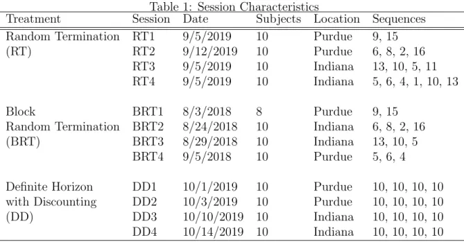
Since there is no money growth, the theoretical steady state inflation rate is zero. To
estimate the inflation rate in the experimental economies, we regress the natural log of the
price level in either market A or B on the time period within sequences. The coefficient
on the time period captures the growth rate of the price level and hence is an estimate of
the inflation rate. Table 2 provides estimates for the inflation rate for each treatment (with
robust standard errors in parentheses), pooling observations from all sessions for the same
treatment. Figure 1 graphs the estimated inflation rates with 95% confidence intervals for
the three treatments. Table 3 lists the estimated inflation rate for each session (see Figure
C.2 in Appendix C for more details on price paths over time, by session and treatment). To facilitate comparison between the three treatments, we also estimate the differences in
inflation rates between each pair of treatments in Table 4. Each entry in a cell represents the
estimate of inflation rate in the row treatment minus inflation rate in the column treatment.
We summarize results on inflation in Finding 1.
Finding 1. Inflation rates in markets A and B are slightly above zero in all three
treatments and not significantly different across treatments.
Table 3 suggests that only two experimental sessions, RT3 and BRT1, exhibit inflation
rates consistent with the theoretical prediction, where both market A and B inflation rates
are not statistically significantly different from zero at the 10% level, and the magnitude is less than half a percent. Most sessions exhibit some mild inflation in either or both markets.
The highest inflation rate is observed in market B in BRT2 at 7.7%, and the lowest in market
B of BRT1, which shows a very mild deflation (although it is not statistically different from
zero).
The regressions in Table 2 suggest the estimated inflation rate is statistically positive for
all treatments, though the magnitudes are moderate. In market A, the estimated average
inflation rate is 2.6% in treatment RT and 3.5% in treatments BRT and DD. In market
B, the estimated inflation is slightly higher than in market A, 4% in treatment RT, 4.7 in
BRT and 6.1% in treatment DD. These magnitudes are also comparable to the constant
money supply treatment of Duffy and Puzzello (2019). In addition, there are no significant
differences across the three treatments as shown in Table 4. We interpret this evidence as
suggesting that inflation in the experimental economies is largely consistent with the steady
Table 2: Inflation Rates in Market A and Market B, by Treatment
Market A Market B
Variables ln(pRTA ) ln(pBRTA ) ln(pDDA ) ln(pRTB ) ln(pBRTB ) ln(pDDB ) Period 0.026∗∗∗ 0.035∗∗∗ 0.035∗∗∗ 0.040∗∗∗ 0.047∗∗∗ 0.061∗∗∗ (0.009) (0.012) (0.012) (0.008) (0.015) (0.013) Constant −1.243∗∗∗ −1.370∗∗∗ −1.041∗∗∗ −1.336∗∗∗ −1.333∗∗∗ −1.126∗∗∗
(0.050) (0.084) (0.071) (0.046) (0.087) (0.077) Observations 134 134 160 134 134 160 R-squared 0.084 0.068 0.054 0.187 0.087 0.148
Notes. (1) Robust standard errors in parentheses. (2) * p-value <0.10, ** p-value< 0.05, *** p-value <0.01.
Table 3: Estimated Inflation by Session
Obs. Market A Inflation Market B Inflation RT1 24 0.073∗∗∗ 0.061∗∗∗ RT2 32 0.018∗ 0.036∗∗∗
RT3 39 0.003 0.001
RT4 39 0.025∗ 0.061∗∗∗
BRT1 25 0.004 -0.005
BRT2 46 0.044∗∗∗ 0.077∗∗∗ BRT3 33 0.025 0.029∗∗ BRT4 30 0.045∗ 0.049 DD1 40 0.039∗∗∗ 0.073∗∗ DD2 40 0.021 0.057∗∗ DD3 40 0.016 0.005∗∗ DD4 40 0.063∗∗∗ 0.064∗∗∗
Notes. (1) Inflation is estimated from regressing ln(Price) on Period for each session. (2) To save space, robust standard errors are omitted. (3) * p-value <0.10, ** p-value <0.05, *** p-value < 0.01.
Table 4: Estimated Difference in Market A and Market B Inflation Market A Inflation Market B Inflation
RT BRT RT BRT
BRT 0.010 0.006 (0.015) (0.017)
DD 0.009 −0.001 0.021 0.014 (0.015) (0.017) (0.015) (0.019)
Figure 1: Estimated Inflation Rates
5.2
Output
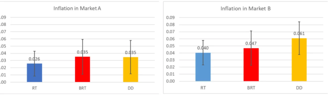
We now discuss output in the experimental economies, focusing on market A because only
the output and consumption in this market affect aggregate welfare, measured as the welfare
ratio in equation (5).17
Table 5 provides summary statistics for period average output across all producers for
each session. Notice that period average output is the same as period average consumption
because we have the same number of producers and consumers. In the analysis below, we
first compare output to the theoretical steady state prediction and summarize the result in
Finding 2. We then discuss treatment effects and summarize them in Finding 3.
Table 5: Average Market A Output-Summary Statistics Session Obs. Mean std.
RT1 24 7.766 2.625 RT2 32 9.938 2.362 RT3 39 8.597 1.783 RT4 39 11.085 2.306 BRT1 25 12.711 2.529 BRT2 46 7.484 3.232 BRT3 33 11.594 3.033 BRT4 30 8.95 2.142 DD1 40 9.426 2.100 DD2 40 8.783 1.912 DD3 40 4.511 1.167 DD4 40 8.023 2.804
Finding 2. Market A output deviate slightly from the steady state prediction in the RT
and BRT treatments and are significantly lower than the steady state prediction in the DD
treatment.
Average output is lower than its steady state prediction of 10 in most experimental
sessions as shown in Table 5. The highest level of output is observed in session BRT1 at
12.711 and the lowest in DD3 at 4.511. Table 6 estimates the deviation of the period average
output from its steady state prediction of 10. In the RT and BRT treatments, the observed output is very close to the steady state prediction. The deviation is -0.508 for RT, and
-0.2 for BRT. In terms of statistical significance, in treatment RT, the deviation of period
average output from the steady state prediction is significant at the 5% level. In treatment
BRT, the period average output is not significantly different from the steady state prediction
at the 10% level. In contrast, period average output in DD is significantly lower than the
steady state prediction in both economic and statistical sense: the deviation is -2.314 and
statistically significant at the 1% level.
Table 6: Average Market A Output Relative to Steady State Prediction Obs. Avg. Market A Output −Steady State
RT 134 −0.508∗∗ (0.220) BRT 134 −0.200 (0.303) DD 160 −2.314∗∗∗
(0.222)
Notes. (1) Robust standard errors are in parentheses. (2)* p-value< 0.10, ** p-value< 0.05, *** p-value <0.01
Finding 3. The period average market A output is not significantly different between the RT and BRT treatments and is significantly lower in DD relative to the other two treatments.
To identify the difference in market A output across the three treatments, we regress the
period market A average output on the two treatment dummies, with robust standard errors.
The constant term from the regression can be interpreted as the estimated market A output
in treatment RT while the coefficients on the two dummy treatment variables correspond to the marginal effect of the two different implementation schemes. The regression results are
provided in Table 7. Figure 2 summarizes the period average output in market A for each
treatment, where the bands correspond to 95% confidence intervals.
Table 7 and Figure 2 show that market A output and consumption are not significantly different between RT and BRT. The regression coefficient on the dummy variable BRT is
statistically insignificant at the 10% significance level. The magnitude of difference is also
Output is lower in treatment DD relative to RT and DD. The period average output and
consumption are 1.807 lower in DD relative to RT, and 2.114 lower relative to BRT. Both
differences are statistically significant at the 1% level. Also note that output is notably lower
in session DD3 relative to other sessions. It appears that subjects coordinated on a lower
level of output in this session. If we remove this session from the regression in Table 7, then
the magnitude of the coefficient on DD decreases from -2.314 to -0.748, though it remains
statistically significant at the 5% level.
Table 7: Regression of Average Market A Output on Treatment Dummies Variables Avg. Market A Output
BRT 0.307
(0.374) DD −1.807∗∗∗
(0.312) Constant 9.492∗∗∗ (0.220) Observations 428 R-squared 0.094
Notes. (1) Robust standard errors are in parentheses. (2)* p-value< 0.10, ** p-value< 0.05, *** p-value <0.01.
Figure 2: Average Market A Output
Finally, we examine the time trend in the average market output and compare the pattern
across the three implementation schemes. For this purpose, we regress the period average
market A output on time period and its interaction terms with the two treatment dummies.
The coefficients for the interaction terms capture the difference in time trend between BRT
Finding 4. Average market A output exhibits a mild negative trend in all three
treat-ments. The difference in time trend across the three treatments is neither statistically nor
economically significant.
Table 8 shows that all three treatments experience mild downward trend in average
market A output. It decreases by about 0.258 per period in treatment RT and slightly less in the other two treatments (see Figure C.1 in Appendix C for more details on average output
patterns over time for each individual session.) Given that the average output is close to the
theoretical prediction (especially for treatments RT and BRT), the slight negative trend may
be attributed in part to the downward adjustment of the initially high output. For example,
the estimated initial average output in treatment RT is 10.999 for treatment RT and 11.27
for treatment BRT.
Table 8: Time Trend in Market A Output and Consumption Variables Avg. Market A Output
Period −0.258∗∗∗ (0.059) Period*BRT 0.024
(0.103) Period*DD 0.020
(0.098)
BRT 0.273
(0.723) DD −2.001∗∗∗
(0.630) Constant 10.999∗∗∗
(0.399) Observations 428 R-squared 0.166
Notes. (1) Robust standard errors are in parentheses. (2)* p-value< 0.10, ** p-value< 0.05, *** p-value <0.01.
5.3
Welfare
In this section, we focus on welfare in the experimental sessions. Table 9 provides summary
statistics for each session. Similar to the analysis on output, we first evaluate whether the
theoretical point prediction describes the experimental sessions well (Table 10 and Finding
5), and then we turn our attention to the differences between the three treatments (Table 12
and Finding 6). Figure 3 reports average welfare ratios across treatments where the bands
Table 9: Welfare Ratio: Summary Statistics by Session and Treatment Session Obs. Mean std.
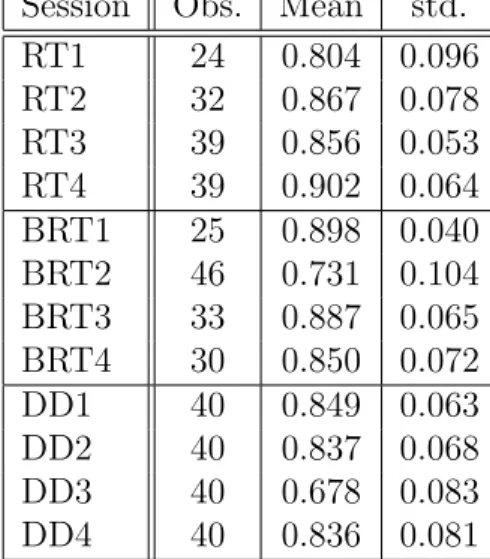
RT1 24 0.804 0.096 RT2 32 0.867 0.078 RT3 39 0.856 0.053 RT4 39 0.902 0.064 BRT1 25 0.898 0.040 BRT2 46 0.731 0.104 BRT3 33 0.887 0.065 BRT4 30 0.850 0.072 DD1 40 0.849 0.063 DD2 40 0.837 0.068 DD3 40 0.678 0.083 DD4 40 0.836 0.081
Finding 5. Welfare is significantly lower than the steady state prediction in all three
treatments.
According to Table 9, the average period welfare ratio is lower than the theoretical
prediction of 0.98 in all 12 experimental economies. The welfare ratio is the highest in session RT4 at 0.902 and the lowest in session DD3 at 0.678. More formally, Table 10 provides
estimates for the deviation of the period welfare ratio from the steady state prediction (0.98)
for each treatment. Welfare is significantly lower in all treatments relative to the theoretical
prediction. Recall the deviation of period average output is not significantly different from
the point prediction in the BRT treatment. The lower welfare relative to the steady state
prediction is partly due to some dispersion of consumption among consumers and across
time.
To measure the extent of consumption dispersion for the three treatments, we calculate
the coefficient of variation for individual consumers’ consumption in market A, which we
report in Table 11. The results suggest that dispersion is greatest in treatment DD, followed
by BRT and finally by RT.
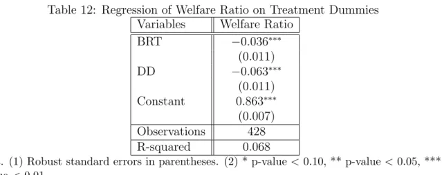
Finding 6. Welfare is significantly lower in BRT and DD relative to RT.
To identify treatment differences, we regress the welfare ratio on treatment dummies and report the results in Table 12. The results from Figure 3 and Table 12 suggest that welfare
is significantly lower in BRT and DD relative to RT. The difference is 0.036 between BRT
and RT, 0.063 between DD and RT, and 0.027 between BRT and DD. The difference in the
first two pairs (last pair) is significant at the 1% (5%) significance level.
con-Table 10: Deviation of Welfare Ratio from Steady State Prediction, by Treatment Obs. Welfare Ratio −0.98
RT 134 −0.116∗∗∗ (0.007) BRT 134 −0.152∗∗∗
(0.009) DD 160 -0.179***
(0.008)
Notes. (1)* p-value <0.10, ** p-value <0.05, *** p-value <0.01.
Table 11: Individual Consumption in Market A: Summary Statistics, by Treatment Treatment Obs. Mean std CoV.
RT 670 9.492 6.197 0.652 BRT 645 9.687 6.763 0.698 DD 900 7.686 5.790 0.753
sumption dispersion also contributes to the difference in welfare ratios across the different
treatments. For example, period average output in BRT is not significantly different from
RT. However, the difference in the welfare ratio is significant at the 1% level.
Figure 3: Welfare Ratio by Treatment
5.4
Discussion
To summarize, we find monetary trade is sustained and dynamic incentives underlying the
theoretical model are broadly preserved in all three implementation schemes. Experimental
outcomes fall within a reasonable neighbourhood of the theoretical prediction. In particular,
treat-Table 12: Regression of Welfare Ratio on Treatment Dummies Variables Welfare Ratio
BRT −0.036∗∗∗ (0.011) DD −0.063∗∗∗
(0.011) Constant 0.863∗∗∗ (0.007) Observations 428 R-squared 0.068
Notes. (1) Robust standard errors in parentheses. (2) * p-value <0.10, ** p-value< 0.05, *** p-value <0.01.
ments. Output is slightly lower than the theoretical prediction in treatments RT and BRT
(and not significantly different between the two), but significantly lower in DD. Welfare is
lower than the theoretical prediction in all treatments, with RT being the closest to theory,
followed by BRT and then DD.
From these findings, can we conclude which method is superior? For the implementation
of infinite horizon models, an important criterion is the preservation of dynamic incentives
underlying the theoretical model. Other more practical criteria include the ease of
im-plementation in the lab and ability of the method to allow for relatively long sessions or
supergames.
Within the context of our experimental monetary economy with constant money
sup-ply, all three methods are able to preserve the dynamic incentives that sustain monetary
trade. The standard random termination method generates behavior closest to theoretical
predictions. The relative superiority, however, is only marginal relative to BRT, and not
overwhelming relative to DD. Given the broad similarity of results among the three meth-ods, one may choose any of the approaches depending on the research questions of interest.
In the following, we discuss the relative advantages of each method.
As for more practical concerns, RT is relatively straightforward to implement compared
with the other two schemes. For instance, one needs to explain additional concepts in BRT (i.e., the block) relative to RT (i.e., only the sequence termination scheme). Indeed in our
case, we were able to run more sequences in the RT treatment relative to BRT. For DD,
one also needs to explain the concept of the continuation value and assess whether subjects
understand the automated calculations. Another advantage of RT is the stake of decisions
is constant over time, while it decreases with the other two; in DD, payoffs are discounted
within the block. If it is mentally challenging to make the right decisions, subjects may have
weaker incentives to do their best in later periods. This concern, however, may be mitigated
by considering the task tends to become easier as subjects gain experience and learn while
the session proceeds.
The BRT design ensures the experimenter observes behavior in a minimum number of periods in each supergame. This could be a useful feature for certain questions. For example,
the literature on price bubbles in experimental asset markets has shown that it takes time
for a bubble to occur. The standard random termination often generates short sequences
that are not informative for the study of this issue. Another example where BRT could be
useful is an inflationary monetary economy, where observing the path of past price changes
would help subjects infer the inflation rate.
There are also benefits associated with the DD method. First, it is not subject to the
credibility criticism on approaches based on random termination since, by design, dynamic
incentives are ensured by the continuation value. Second, the fixed rounds of decision making
in DD facilitates comparison between different supergames, sessions and treatments. Third, if
the experimenter needs to collect data on multiple supergames for settings with high discount
factors, the DD method may be desirable as one can control the length of the fixed horizon.
Some research questions need to use a within subjects design that runs supergames featuring different treatments in the same session. For example, to study the adoption and usage of a
new currency or a means of payment, one may need to run at least three supergames: the
first with only the existing currency, the second with a new currency alongside the existing
currency, and then a third one repeating the second to investigate whether the first-mover
advantage will weaken or disappear over time.
6
Conclusions
The implementation of infinite-horizon models often relies on random termination which
interprets the discount factor as the probability the game continues to the next period. This
approach is subject to the criticism that it is challenging for the experimenter to credibly
im-plement a game that lasts an arbitrarily long time given the limited length of an experimental
session.
In this paper, we propose a new implementation scheme to address such credibility issues.
In our proposed scheme, subjects play a game for a fixed number of periods and the discount
are preserved by paying subjects a continuation value based on prior outcomes. We apply
our proposed scheme in an infinite horizon monetary economy and compare outcomes with
two commonly used implementations based on random termination.
We find dynamic incentives are preserved and behavior is similar in all three
implemen-tations. Given the broad similarity of results among the three methods, one may choose any of the approaches depending on the research question of interest and more practical
criteria, such as the ease of implementation in the lab and the ability of the method to allow
for relatively more or longer supergames. For instance, RT is relatively easy to explain to
subjects and implement in the lab while BRT ensures each supergame has a minimum
num-ber of periods, which makes it particularly useful for research questions where having have
sufficiently large number periods per sequence or supergame is important. The benefit of
DD is that one can control the length of the fixed horizon, which makes it easier to conduct
within-subjects treatments in the same session when the underlying game involves a high
discount factor.
Our study contributes to the experimental literature by comparing different
infinite-horizon implementation methods in the context of a monetary economy. Our DD approach
can also be modified to enrich the random termination approach commonly adopted in the
laboratory with discounting. For example, in the event the economy is still going on and the recruitment time has come to an end, the experimenter could invoke the interpretation
of β as the discount factor, compute the continuation value and pay subjects accordingly. This adaptation blends the random termination and discounting interpretations. Our new
method can also be adapted for the implementation of infinitely repeated prisoner dilemma
games. We plan to pursue this implementation in future research. Another avenue for future
research is to consider an implementation along the lines proposed by Lim, Prescott, and
Sunder (1986) and Marimon and Sunder (1993), where additional subjects are recruited to
elicit forecast for future prices.
References
Aliprantis, C., G. Camera and D. Puzzello (2007). “Contagion Equilibria in a Monetary
Model.” Econometrica, 75 (1), 277-282.
Araujo, L. (2004). “Social Norms and Money.”Journal of Monetary Economics, 51,
241-256.
Experimental Evidence from Multi-Stage Games.” Journal of Economic Behavior and
Or-ganization, 81(1), 207–219.
Arifovic, J. (1996). ”The Behavior of the Exchange Rate in the Genetic Algorithm and
Experimental Economies.” Journal of Political Economy, 104, 510–541.
Battaglini, M., S. Nunnari and T. Palfrey (2012). “Legislative Bargaining and the
Dy-namics of Public Investment.”American Political Science Review, 106, 407-429.
Battaglini, M., S. Nunnari and T. Palfrey (2016). “The Dynamic Free Rider Problem:
A Laboratory Study.”American Economic Journal: Microeconomics, 8, 268–308.
Bernasconi, M. and O. Kirchkamp (2000). “Why do monetary policies matter? An experimental study of saving and inflation in an overlapping generations model.” Journal of
Monetary Economics, 46, 315–343.
Camera, G. and M. Casari (2014). “The Coordination Value of Monetary Exchange:
Experimental Evidence.” American Economic Journal: Microeconomics, 6, 629–660.
Camera, G., M. Casari, and S. Bortolotti (2016). “An Experiment on Retail Payment
Systems.” Journal of Money, Credit, and Banking, 48, 363–392.
Cooper, D. and K. Kuhn (2014). “Communication, Renegotiation, and the Scope for
Collusion.” American Economic Journal: Microeconomics, 6(2), 247-278.
Dal B´o, P. and G. Fr´echette (2011). “The Evolution of Cooperation in Infinitely Repeated
Games: Experimental Evidence.”American Economic Review, 101, 411-429.
Dal B´o, P. and G. Fr´echette (2018). “On the Determinants of Cooperation in Infinitely
Repeated Games: A survey.”Journal of Economic Literature, 56 (1), 60-114.
Davis, D., O. Korenok, P. Norman, B. Sultanum and R. Wright (2019). “Playing with
Money.” Working Paper.
Ding, S. and D. Puzzello (2019). “Legal Restrictions and International Currencies: An
Experimental Approach,” Mimeo.
Duffy, J. (1998). “Monetary Theory in the Laboratory.” Federal Reserve Bank of St.
Louis, Economic Review, 9–26.
Duffy, J. (2016). “Macroeconomics: A Survey of Laboratory Research,” in: J.H. Kagel
and A.E. Roth (Eds.), Handbook of Experimental Economics Volume 2, Princeton: Prince-ton University Press, 1-90.
Duffy, J., Jiang, J., Xie, H. (2019). “Experimental Asset Markets with An
http://dx.doi.org/10.2139/ssrn.3420184
Duffy, J., A. Matros, and T. Temzelides (2011). “Competitive Behavior in Market Games:
Evidence and Theory.” Journal of Economic Theory, 146, 1437-1463.
Duffy, J. and J. Ochs (1999). “Emergence of Money as a Medium of Exchange: An
Experimental Study.” American Economic Review, 89(4): 847–877.
Duffy, J. and J. Ochs (2002). “Intrinsically Worthless Objects as Media of Exchange:
Experimental Evidence.” International Economic Review, 43, 637–673.
Duffy, J. and D. Puzzello (2014a). “Gift Exchange versus Monetary Exchange: Experi-mental Evidence.” American Economic Review, 104(6), 1735–1776.
Duffy, J. and D. Puzzello (2014b). ”Experimental Evidence on the Essentiality and Neutrality of Money in a Search Model.” Experiments in Macroeconomics, Research in
Ex-perimental Economics, 17, Emerald.
Fischbacher, U. (2007). “Z-Tree: Toolbox for Ready-Made Economic Experiments.”
Experimental Economics, 10, 171–178.
Jiang, J., D. Puzzello, and C. Zhang (2020). “Inflation and Welfare in the Laboratory.”
Mimeo.
Jiang, J. and C. Zhang (2018). “Competing currencies in the laboratory.” Journal of Economic Behavior and Organization, 154, 253-280.
Kamiya, K., H. Kobayashi, T. Shichijo, and T. Shimizu (2019). “Efficiency of Monetary
Exchange with Divisible fiat Money: An experimental Approach,” Mimeo.
Lagos, R. and R. Wright (2005). “A Unified Framework for Monetary Theory and Policy
Analysis.” Journal of Political Economy, 113(3), 463–486.
Lim, S., E. Prescott, and S. Sunder (1986). “Stationary Solution to the Overlapping
Generations Model of Fiat Money: Experimental Evidence,” Mimeo.
Mailath, G. and L. Samuelson (2006). Repeated Games and Reputations:Long-Run Re-lationships, Oxford University Press.
Marimon, R. and S. Sunder (1993). “Indeterminacy of Equilibria in a Hyperinflationary
World: Experimental Evidence.” Econometrica, 61(5), 1073-1107.
Matsuyama, K., N. Kiyotaki, and A. Matsui (1993). “Toward a Theory of International
Currency.” Review of Economic Studies, 60, 283–307.
McCabe, K. (1989). “Fiat Money as a Store of Value in an Experimental Market.”
Osborne, M. and A. Rubinstein (1994). A Course in Game Theory, MIT Press.
Rietz, J. (2019). “Secondary Currency Acceptance: Experimental Evidence with a Dual
Currency Search Model.” Journal of Economic Behavior and Organization, 166, 403-431.
Rocheteau, Guillaume and Ed Nosal (2017). Money, Payments and Liquidity, MIT Press.
Rocheteau, G. and R. Wright (2005). ”Money in Search Equilibrium, in Competitive
Equilibrium, and in Competitive Search Equilibrium.” Econometrica 73, 175-202.
Romero, J. and Y. Rosokha (2018). “Constructing Strategies in the Indefinitely Repeated
Prisoner’s Dilemma Game.” European Economic Review, 104, 185-219.
Roth, A. and K. Murnighan (1978). “Equilibrium Behavior and Repeated Play of the
Prisoner’s Dilemma.” Journal of Mathematical Psychology, 17(2), 189–198.
Sabater-Grande, G. and N. Georgantzis (2002). “Accounting for Risk Aversion in
Re-peated prisoners’ Dilemma Games: An experimental test.” Journal of Economic Behavior
and Organization, 48(1), 37–50.
Selten, R., M. Mitzkewitz, and G. Uhlich (1997). “Duopoly Strategies Programmed by
Experienced Players.” Econometrica, 65 (3), 517-555.
Selten, R. and R. Stoecker (1986). “End Behavior in Sequences of Finite Prisoner’s
Dilemma Supergames.” Journal of Economic Behavior and Organization, 7, 47-70.
Shapley, L., and M. Shubik (1977). “Trade Using One Commodity as a Means of
Pay-ment.” Journal of Political Economy, 85, 937-968.
Wilson, A. and H. Wu (2017). “At-will relationships: How an option to walk away affects
A
Steady State Monetary Equilibrium
We focus on stationary equilibria where real variables are constant over time. Because money supply is constant, the price level is also constant over time. In the analysis below, we omit
the time subscript and use “∧” to denote variables in the next period. As is standard, we
start backwards by characterizing agents’ decision problems in market B and combine that
with choices in market A to characterize the equilibrium.
Market B Decision Problems
In market B, agents can trade good B and money in a competitive market where the price of good B is pB. The value function of an type i agent who enters market B with money
holdingsmi is
max
ˆ
mi,xi B
Wi(mi) = max
ˆ
mi,xi B
−xiB+vi+βVi( ˆmi) subject to ˆmi = pBxB+mi,
where vA = 0, vB = v
0, and ˆmi is the choice of money holdings in the next market A.
Substituting the budget constraint into the objective, the value function simplifies to
max
ˆ
mi W
i
(mi) = max
ˆ
mi
−
ˆ
mi+mi
pB
+βVi( ˆmi)
.
The optimal choice for ˆmi solves
β∂V
i( ˆmi)
∂mˆi −
1
pB
≤0, with equality if ˆmi >0.
As is usual, the value functionWi(m) is linear inm, and the choice of money holdings next period ˆm is independent of current money holdings. The envelope result for both types of agents is
∂Wi(m)
∂m =
1
pB
.
Market A Decision Problems
Agents in market A can trade good A and money in a competitive market at market price
xA units of good A. Their decision problem is
VB(m) = max
xA
−xA+
(m+xApA)
pB
+WB(0)
.
Notice that we have used the envelope result ∂W∂mi(m) = p1
B. The first-order condition of type
B’s problem implies
pA=pB. (A.1)
The envelope result is
∂VB(m)
∂mˆ = 1
pB
.
Type A agents, who are consumers in market A, can buy and consume xA units of good
A. Their value function in market A is
VA(m) = max
xA
u(xA) +
(m−pA)xA
pB)
+WA(0)
subject to pAxA ≤ m.
If the cash constraint does not bind, thenu0(xA) =pA/pB, which when combined with type
B’s decision, gives xA = x∗A. If the cash constraint binds, then xA = m/pA. In either case,
the envelope condition is
∂VA(m)
∂m =
u0(xA)
pA
.
Equilibrium
We now combine agents’ decision problems from market A and B to derive the equations
that characterize the stationary monetary equilibrium. For type B agents, the net marginal
value of carrying money to the next market A is
− 1
pB
+β∂V
B( ˆm)
∂mˆ = − 1
pB
+β 1
ˆ
pB
= 1
pB
[−1 +β]<0.
In words, the money carried by type B agents to market A will be idle in market A and
can be used to purchase good B in the next market B. Given β <1, holding idle balances is costly. As a result, type B agents will spend all money in market B and enter market A
For type A agents, the net marginal value of carrying money to the next market A is
− 1
pB
+β∂V
A( ˆm)
∂mˆ = − 1
pB
+βu
0(x
A)
ˆ
pA
=− 1
pB
+β(1 +τ)u
0(x
A)
ˆ
pB
= 1
pB
[−1 +βu0(xA)].
Under the assumption u0(0) =∞, type A agents hold positive amount of money to market A, and in equilibrium, the net marginal benefit of carrying money is zero, and output in
market A (per consumer or producer) is
u0(xA) = 1/β. (A.2)
Given β < 1, agents will carry just enough money to spend in market A and the cash constraint will bind in market A.
In market A, each type A consumes xA and each type B produces xA, where xA solves
equation (A.2). The price level, which is the same for both markets according to equation
(A.1), is given by the money market clearing condition
pA =pB =
M N xA
. (A.3)
In market B, the amount of consumption by each type B agent (which is the same as
production by each type A agent) is
xB =
M N pB
= M
N pA